On Smoothed Analysis of Quicksort and Hoare’s Find

Abstract

Abstract.  We provide a smoothed analysis of Hoare’s find algorithm and we revisit the smoothed analysis of quicksort.

Hoare’s find algorithm – often called quickselect – is an easy-to-implement algorithm for finding the $k$-th smallest element of a sequence. While the worst-case number of comparisons that Hoare’s find needs is $\Theta(n^{2})$, the average-case number is $\Theta(n)$. We analyze what happens between these two extremes by providing a smoothed analysis of the algorithm in terms of two different perturbation models: additive noise and partial permutations.

In the first model, an adversary specifies a sequence of $n$ numbers of $[0,1]$, and then each number is perturbed by adding a random number drawn from the interval $[0,d]$. We prove that Hoare’s find needs $\Theta\bigl{(}\frac{n}{d+1}\sqrt{n/d}+n\bigr{)}$ comparisons in expectation if the adversary may also specify the element that we would like to find. Furthermore, we show that Hoare’s find needs fewer comparisons for finding the median.

In the second model, each element is marked with probability $p$ and then a random permutation is applied to the marked elements. We prove that the expected number of comparisons to find the median is $\Omega\bigl{(}(1-p)\frac{n}{p}\log n\bigr{)}$, which is again tight.

Finally, we provide lower bounds for the smoothed number of comparisons of quicksort and Hoare’s find for the median-of-three pivot rule, which usually yields faster algorithms than always selecting the first element: The pivot is the median of the first, middle, and last element of the sequence. We show that median-of-three does not yield a significant improvement over the classic rule: the lower bounds for the classic rule carry over to median-of-three.

1 Introduction

To explain the discrepancy between average-case and worst-case behavior of the simplex algorithm, Spielman and Teng introduced the notion of smoothed analysis [18]. Smoothed analysis interpolates between average-case and worst-case analysis: Instead of taking a worst-case instance, we analyze the expected worst-case running time subject to slight random perturbations. The more influence we allow for perturbations, the closer we come to the average case analysis of the algorithm. Therefore, smoothed analysis is a hybrid of worst-case and average-case analysis.

In practice, neither can we assume that all instances are equally likely, nor that instances are precisely worst-case instances. The goal of smoothed analysis is to capture the notion of a typical instance mathematically. Typical instances are, in contrast to worst-case instances, often subject to measurement or rounding errors. Even if one assumes that nature is adversarial and that the instance at hand was initially a worst-case instance, due to such errors we would probably get a less difficult instance in practice. On the other hand, typical instances still have some (adversarial) structure, which instances drawn completely at random do not. Spielman and Teng [19] give a survey of results and open problems in smoothed analysis.

In this paper, we provide a smoothed analysis of Hoare’s find [7] (see also Aho et al. [1, Algorithm 3.7]), which is a simple algorithm for finding the $k$-th smallest element of a sequence of numbers: Pick the first element as the pivot and compare it to all $n-1$ remaining elements. Assume that $\ell-1$ elements are smaller than the pivot. If $\ell=k$, then the pivot is the element that we are looking for. If $\ell>k$, then we recurse to find the $k$-th smallest element of the list of the smaller elements. If $\ell<k$, then we recurse to find the $(k-\ell)$-th smallest element among the larger elements. The number of comparisons to find the specified element is $\Theta(n^{2})$ in the worst case and $\Theta(n)$ on average. Furthermore, the variance of the number of comparisons is $\Theta(n^{2})$ [8]. As our first result, we close the gap between the quadratic worst-case running-time and the expected linear running-time by providing a smoothed analysis.

Hoare’s find is closely related to quicksort [6] (see also Aho et al. [1, Section 3.5]), which needs $\Theta(n^{2})$ comparisons in the worst case and $\Theta(n\log n)$ on average [10, Section 5.2.2]. The smoothed number of comparisons that quicksort needs has already been analyzed [12]. Choosing the first element as the pivot element, however, results in poor running-time if the sequence is nearly sorted. There are two common approaches to circumvent this problem: First, one can choose the pivot randomly among the elements. However, randomness is needed to do so, which is sometimes expensive. Second, without any randomness, a common approach to circumvent this problem is to compute the median of the first, middle, and last element of the sequence and then to use this median as the pivot [17, 16]. This method is faster in practice since it yields more balanced partitions and it makes the worst-case behavior much more unlikely [10, Section 5.5]. It is also faster both in average and in worst case, albeit only by constant factors [5, 15]. Quicksort with the median-of-three rule is widely used, for instance in the qsort() implementation in the GNU standard C library glibc library [14] and also in a recent very efficient implementation of quicksort on a GPU [3]. The median-of-three rule has also been used for Hoare’s find, and the expected number of comparisons has been analyzed precisely [9].

Our second goal is a smoothed analysis of both quicksort and Hoare’s find with the median-of-three rule to get a thorough understanding of this variant of these two algorithms.

1.1 Preliminaries

We denote sequences of real numbers by $s=(s_{1},\ldots,s_{n})$, where $s_{i}\in\mathbb{R}$. For $n\in{\rm Nature}$, we set $[n]=\{1,\ldots,n\}$. Let $U=\{i_{1},\ldots,i_{\ell}\}\subseteq[n]$ with $i_{1}<i_{2}<\ldots<i_{\ell}$. Then $s_{U}=(s_{i_{1}},s_{i_{2}},\ldots,s_{i_{\ell}})$ denotes the subsequence of $s$ of the elements at positions in $U$. We denote probabilities by $\mathbb{P}$ and expected values by $\mathbb{E}$.

Throughout the paper, we will assume for the sake of clarity that numbers like $\sqrt{d}$ are integers and we do not write down the tedious floor and ceiling functions that are actually necessary. Since we are interested in asymptotic bounds, this does not affect the validity of the proofs.

Pivot Rules.

Given a sequence $s$, a pivot rule simply selects one element of $s$ as the pivot element. The pivot element will be the one to which we compare all other elements of $s$. In this paper, we consider four pivot rules, two of which play only a helper role (the acronyms of the rules are in parentheses):

Classic rule (c):

The first element $s_{1}$ of $s$ is the pivot element.

Median-of-three rule (m3):

The median of the first, middle, and last element is the pivot element, i.e., $\operatorname{median}(s_{1},s_{\lceil n/2\rceil},s_{n})$.

Maximum-of-two rule (max2):

The maximum of the first and the last element becomes the pivot element, i.e., $\max(s_{1},s_{n})$.

Minimum-of-two rule (min2):

The minimum of the first and the last element becomes the pivot element, i.e., $\min(s_{1},s_{n})$.

The first pivot rule is the easiest-to-analyze and easiest-to-implement pivot rule for quicksort and Hoare’s find. Its major drawback is that it yields poor running-times of quicksort and Hoare’s find for nearly sorted sequences. The advantages of the median-of-three rule has already been discussed above. The last two pivot rules are only used as tools for analyzing the median-of-three rule.

Quicksort, Hoare’s Find, Left-to-right Maxima.

Let $s$ be a sequence of length $n$ consisting of pairwise distinct numbers. Let $p$ be the pivot element of $s$ according to some rule. For the following definitions, let $L=\{i\in\{1,\dots,n\}\mid s_{i}<p\}$ be the set of positions of elements smaller than the pivot, and let $R=\{i\in\{1,\dots,n\}\mid s_{i}>p\}$ be the set of positions of elements greater than the pivot.

Quicksort is the following sorting algorithm: Given $s$, we construct $s_{L}$ and $s_{R}$ by comparing all elements to the pivot $p$. Then we sort $s_{L}$ and $s_{R}$ recursively to obtain $s^{\prime}_{L}$ and $s^{\prime}_{R}$, respectively. Finally, we output $s^{\prime}=(s^{\prime}_{L},p,s^{\prime}_{R})$. The number $\operatorname{sort}(s)$ of comparisons needed to sort $s$ is thus $\operatorname{sort}(s)=(n-1)+\operatorname{sort}(s_{L})+\operatorname{sort}(s_{R})$ if $s$ has a length of $n\geq 1$, and $\operatorname{sort}(s)=0$ when $s$ is the empty sequence. We do not count the number of comparisons needed to find the pivot element. Since this number is $O(1)$ per recursive call for the pivot rules considered here, this does not change the asymptotics.

Hoare’s find aims at finding the $k$-th smallest element of $s$. Let $\ell=|s_{L}|$. If $\ell=k-1$, then $p$ is the $k$-th smallest element. If $\ell\geq k$, then we search for the $k$-th smallest element of $s_{L}$. If $\ell<k-1$, then we search for the $(k-\ell)$-th smallest element of $s_{R}$. Let $\operatorname{find}(s,k)$ denote the number of comparisons needed to find the $k$-th smallest element of $s$, and let $\operatorname{find}(s)=\max_{k\in[n]}\operatorname{find}(s,k)$.

The number of scan maxima of $s$ is the number of maxima seen when scanning $s$ according to some pivot rule: let $\operatorname{scan}(s)=1+\operatorname{scan}(s_{R})$, and let $\operatorname{scan}(s)=0$ when $s$ is the empty sequence. If we use the classic pivot rule, the number of scan maxima is just the number of left-to-right maxima, i.e., the number of new maxima that we see if we scan $s$ from left to right. The number of scan maxima is a useful tool for analyzing quicksort and Hoare’s find, and has applications, e.g., in motion complexity [4].

We write $\operatorname{c-scan}(s)$, $\operatorname{m3-scan}(s)$, $\operatorname{max2-scan}(s)$, and $\operatorname{min2-scan}(s)$ to denote the number of scan maxima according to the classic, median-of-three, maximum, or minimum pivot rule, respectively. Similar notation is used for quicksort and Hoare’s find.

Perturbation Model: Additive noise.

The first perturbation model that we consider is additive noise. Let $d>0$. Given a sequence $s\in[0,1]^{n}$, i.e., the numbers $s_{1},\ldots,s_{n}$ lie in the interval $[0,1]$, we obtain the perturbed sequence $\overline{s}=(\overline{s}_{1},\ldots,\overline{s}_{n})$ by drawing $\nu_{1},\ldots,\nu_{n}$ uniformly and independently from the interval $[0,d]$ and setting $\overline{s}_{i}=s_{i}+\nu_{i}$. Note that $d=d(n)$ may be a function of the number $n$ of elements, although this will not always be mentioned explicitly in the following.

We denote by $\operatorname{scan}_{d}(s)$, $\operatorname{sort}_{d}(s)$ and $\operatorname{find}_{d}(s)$ the (random) number of scan maxima, quicksort comparisons, and comparisons of Hoare’s find of $\overline{s}$, preceded by the acronym of the pivot rule used.

Our goal is to prove bounds for the smoothed number of comparisons that Hoare’s find needs, i.e., $\max_{s\in[0,1]^{n}}\mathbb{E}\bigl{(}\operatorname{c-find}_{d}(s)\bigr{)}$, as well as for Hoare’s find and quicksort with the median-of-three pivot rule, i.e., $\max_{s\in[0,1]^{n}}\mathbb{E}\bigl{(}\operatorname{m3-find}_{d}(s)\bigr{)}$ and $\max_{s\in[0,1]^{n}}\mathbb{E}\bigl{(}\operatorname{m3-sort}_{d}(s)\bigr{)}$. The $\max$ reflects that the sequence $s$ is chosen by an adversary.

If $d<1/n$, the sequence $s$ can be chosen such that the order of the elements is unaffected by the perturbation. Thus, in the following, we assume $d\geq 1/n$. If $d$ is large, the noise will swamp out the original instance, and the order of the elements of $\overline{s}$ will basically depend only on the noise rather than the original instance. For intermediate $d$, we interpolate between the two extremes.

The choice of the intervals for the adversarial part and the noise is arbitrary. All that matters is the ratio of the sizes of the intervals: For $a<b$, we have $\max_{s\in[a,b]^{n}}\mathbb{E}\bigl{(}\operatorname{find}_{d\cdot(b-a)}(s)\bigr{)}=\max_{s\in[0,1]^{n}}\mathbb{E}\bigl{(}\operatorname{find}_{d}(s)\bigr{)}$. In other words, we can scale (and also shift) the intervals, and the results depend only on the ratio of the interval sizes and the number of elements. The same holds for all other measures that we consider. We will exploit this in the analysis of Hoare’s find.

Perturbation Model: Partial Permutations.

The second perturbation model that we consider is partial permutations, introduced by Banderier, Beier, and Mehlhorn [2]. Here, the elements are left unchanged. Instead, we permute a random subsets of the elements.

Without loss of generality, we can assume that $s$ is a permutation of a set of $n$ numbers, say, $\{1,\ldots,n\}$. The perturbation parameter is $p\in[0,1]$. Any element $s_{i}$ (or, equivalently, any position $i$) is marked independently of the others with a probability of $p$. After that, all marked positions are randomly permuted: Let $M$ be the set of positions that are marked, and let $\pi:M\to M$ be a permutation drawn uniformly at random. Then

$$\overline{s}_{i}=\begin{cases}s_{\pi(i)}&\text{if $i\in M$ and}\\ s_{i}&\text{otherwise.}\end{cases}$$

If $p=0$, no element is marked, and we obtain worst-case bounds. If $p=1$, all elements are marked, and $\overline{s}$ is a uniformly drawn random permutation.

1.2 Known Results

Additive noise is perhaps the most basic and natural perturbation model for smoothed analysis. In particular, Spielman and Teng added random numbers to the entries of the adversarial matrix in their smoothed analysis of the simplex algorithm [18]. Damerow, Meyer auf der Heide, Räcke, Scheideler, and Sohler [4] analyzed the smoothed number of left-to-right maxima of a sequence under additive noise. They obtained upper bounds of $O\big{(}\sqrt{\frac{n}{d}\log n}+\log n\big{)}$ for a variety of distributions and a lower bound of $\Omega(\sqrt{n}+\log n)$. Manthey and Tantau tightened their bounds for uniform noise to $O\big{(}\sqrt{n/d}+\log n\big{)}$. Furthermore, they proved that the same bounds hold for the smoothed tree height. Finally, they showed that quicksort needs $O\big{(}\frac{n}{d+1}\cdot\sqrt{\frac{n}{d}}\big{)}$ comparisons in expectation, and this bound is also tight [12].

Banderier et al. [2] introduced partial permutations as a perturbation model for ordering problems like left-to-right maxima or quicksort. They proved that a sequence of $n$ numbers has, after partial permutation, an expected number of $O\big{(}\sqrt{\frac{n}{p}\log n}\big{)}$ left-to-right maxima, and they proved a lower bound of $\Omega\bigl{(}\sqrt{n/p}\bigr{)}$ for $p\leq\frac{1}{2}$. This has later been tightened by Manthey and Reischuk [11] to $\Theta\bigl{(}(1-p)\cdot\sqrt{n/p}\bigr{)}$. They transferred this to the height of binary search trees, for which they obtained the same bounds. Banderier et al. [2] also analyzed quicksort, for which they proved an upper bound of $O\big{(}\frac{n}{p}\log n\big{)}$.

1.3 New Results

We give a smoothed analysis of Hoare’s find under additive noise. We consider both finding an arbitrary element and finding the median. First, we analyze finding arbitrary elements, i.e., the adversary specifies $k$, and we have to find the $k$-th smallest element (Section 2). For this variant, we prove tight bounds of $\Theta\bigl{(}\frac{n}{d+1}\sqrt{n/d}+n\bigr{)}$ for the expected number of comparisons. This means that already for very small $d\in\omega(1/n)$, the smoothed number of comparisons is reduced compared to the worst case. If $d$ is a small constant, i.e., the noise is a small percentage of the data values like $1\%$, then $O(n^{3/2})$ comparisons suffice.

If the adversary is to choose $k$, our lower bound suggests that we will have either $k=1$ or $k=n$. The main task of Hoare’s find, however, is to find medians. Thus, second, we give a separate analysis of how much comparisons are needed to find the median (Section 3). It turns out that under additive noise, finding medians is arguably easier than finding maximums or minimums: For $d\leq 1/2$, we have the same bounds as above. For $d\in(\frac{1}{2},2)$, we prove a lower bound of $\Omega\bigl{(}n^{3/2}\cdot(1-\sqrt{d/2})\bigr{)}$, which again matches the upper bound of Section 2, which of course still applies (Section 3.1). For $d>2$, we prove that a linear number of comparisons suffices, which is considerably less than the $\Omega\bigl{(}(n/d)^{3/2}\bigr{)}$ general lower bound of Section 2. For the special value $d=2$, we prove a tight bound of $\Theta(n\log n)$ (Sections 3.3 and 3.4).

After that, we aim at analyzing different pivot rules, namely the median-of-three rule. As a tool, we analyze the number of scan maxima under the maximum-of-two, minimum-of-two, and median-of-three rule (Section 4). We essentially show that the same bounds as for the classic rule carry over to these rules. Then we apply these findings to quicksort and Hoare’s find (Section 5). Again, we prove a lower bound that matches the lower bound for the classic rule. Thus, the median-of-three does not seem to help much under additive noise.

The results concerning additive noise are summarized in Table 1.

algorithm	$d\leq 1/2$	$d\in(1/2,2)$	$d=2$	$d>2$
quicksort (c)	$\Theta\bigl{(}n\sqrt{n/d}\bigr{)}$	$\Theta\bigl{(}n^{3/2}\bigr{)}$	$\Theta\bigl{(}n^{3/2}\bigr{)}$	$\Theta\bigl{(}(n/d)^{3/2}\bigr{)}$
quicksort (m3)	$\Omega\bigl{(}n\sqrt{n/d}\bigr{)}$	$\Omega\bigl{(}n^{3/2}\bigr{)}$	$\Omega\bigl{(}n^{3/2}\bigr{)}$	$\Omega\bigl{(}(n/d)^{3/2}\bigr{)}$
Hoare’s find (median, c)	$\Theta\bigl{(}n\sqrt{n/d}\bigr{)}$	$\Omega\bigl{(}n^{3/2}(1-\sqrt{d/2})\bigr{)}$	$\Theta(n\log n)$	$O\bigl{(}\frac{d}{d-2}\cdot n\bigr{)}$
Hoare’s find (general, c)	$\Theta\bigl{(}n\sqrt{n/d}\bigr{)}$	$\Theta\bigl{(}n^{3/2}\bigr{)}$	$\Theta\bigl{(}n^{3/2}\bigr{)}$	$\Theta\bigl{(}(n/d)^{3/2}\bigr{)}$
Hoare’s find (general, m3)	$\Theta\bigl{(}n\sqrt{n/d}\bigr{)}$	$\Theta\bigl{(}n^{3/2}\bigr{)}$	$\Theta\bigl{(}n^{3/2}\bigr{)}$	$\Theta\bigl{(}(n/d)^{3/2}\bigr{)}$
scan maxima (c)	$\Theta\bigl{(}\sqrt{n/d}\bigr{)}$	$\Theta\bigl{(}\sqrt{n}\bigr{)}$	$\Theta\bigl{(}\sqrt{n}\bigr{)}$	$\Theta\bigl{(}\sqrt{n/d}\bigr{)}$
scan maxima (m3)	$\Theta\bigl{(}\sqrt{n/d}\bigr{)}$	$\Theta\bigl{(}\sqrt{n}\bigr{)}$	$\Theta\bigl{(}\sqrt{n}\bigr{)}$	$\Theta\bigl{(}\sqrt{n/d}\bigr{)}$

Table 1: Overview of bounds for additive noise. The bounds for quicksort and scan maxima with classic pivot rule are by Manthey and Tantau [12]. The upper bounds for Hoare’s find in general apply also to Hoare’s find for finding the median. Note that, even for large $d$, the precise bounds for quicksort, Hoare’s find, and scan maxima never drop below $\Omega(n\log n)$, $\Omega(n)$, and $\Omega(\log n)$, respectively.

Finally, and to contrast our findings for additive noise, we analyze Hoare’s find under partial permutations (Section 6). We prove that there exists a sequence on which Hoare’s find needs an expected number of $\Omega\bigl{(}(1-p)\cdot\frac{n}{p}\cdot\log n\bigr{)}$ comparisons. Since this matches the upper bound for quicksort [2] up to a factor of $O(1-p)$, this lower bound is essentially tight.

For completeness, Table 2 gives an overview of the results for partial permutations.

algorithm	bound
quicksort	$O\bigl{(}(n/p)\log n\bigr{)}$
Hoare’s find	$\Omega\bigl{(}(1-p)(n/p)\log n\bigr{)}$
scan maxima	$\Theta\bigl{(}(1-p)\sqrt{n/p}\bigr{)}$
binary search trees	$\Theta\bigl{(}(1-p)\sqrt{n/p}\bigr{)}$

Table 2: Overview of bounds for partial permutations. All results are for the classic pivot rule. The results about quicksort, scan maxima, and binary search trees are by Banderier et al. [2] and Manthey and Reischuk [11]. The upper bound for quicksort also holds for Hoare’s find, while the lower bound for Hoare’s find also applies to quicksort.

2 Smoothed Analysis of Hoare’s Find: General Bounds

In this section, we prove tight bounds for the smoothed number of comparisons that Hoare’s find needs using the classic pivot rule.

Theorem 2.1.

For $d\geq 1/n$, we have

$$\max_{s\in[0,1]^{n}}\mathbb{E}\bigl{(}\operatorname{c-find}_{d}(s)\bigr{)}\in\Theta\bigl{(}\textstyle\frac{n}{d+1}\sqrt{n/d}+n\bigr{)}.$$

The following subsection contains the proof of the upper bound. After that, we prove the lower bound.

2.1 General Upper Bound for Hoare’s Find

We already have an upper bound for the smoothed number of comparisons that quicksort needs [12]. This bound is $O\bigl{(}\frac{n}{d+1}\cdot\sqrt{n/d}+n\log n\bigr{)}$, which matches the bound of Theorem 2.1 for $d\in O\bigl{(}n^{1/3}\cdot\log^{-2/3}n\bigr{)}$. We have $\operatorname{find}(s)\leq\operatorname{sort}(s)$ for any $s$. By monotonicity of the expectation, this inequality yields $\mathbb{E}\bigl{(}\operatorname{find}_{d}(s)\bigr{)}\leq\mathbb{E}\bigl{(}\operatorname{sort}_{d}(s)\bigr{)}$. Thus, $d\in\Omega\bigl{(}n^{1/3}\cdot\log^{-2/3}n\bigr{)}$ remains to be analyzed.

In the next lemma, we show how to analyze the number of comparisons in terms of subsequences. Lemma 2.3 states that adding a single element to a sequence increases the number of comparisons at most by an additive $O(n)$. Lemma 2.4 states the actual upper bound.

Lemma 2.2.

Let $s$ be a sequence, and let $k\in[n]$. Let $j$ be the position of the $k$-th smallest element of $s$. Let $U_{1},\ldots,U_{m}$ be a covering of $[n]$, i.e., $\bigcup_{\ell=1}^{m}U_{\ell}=[n]$, such that $j\in U_{\ell}$ for all $\ell\in[m]$. Let $k_{1},\ldots,k_{m}$ be chosen such that $s_{j}$ is the $k_{\ell}$-th smallest element of $s_{U_{\ell}}$. Then

$$\operatorname{find}(s,k)\leq\sum_{\ell=1}^{m}\operatorname{find}(s_{U_{\ell}},k_{\ell})+Q,$$

where $Q$ is the number of comparisons of positions $a$ and $b$ in $\operatorname{find}(s,k)$ such that $a$ and $b$ do not share a common set in the covering, i.e., $\{a,b\}\not\subseteq U_{\ell}$ for all $\ell\in[m]$.

Proof.

Fix any $\ell\in[m]$, and let $a$ and $b$ be two elements of $s_{U_{\ell}}$ that are not compared for finding the $k_{\ell}$-th smallest element of $U_{\ell}$. Without loss of generality, we assume that $a<b$ and that $a$ appears before $b$ in $s_{U_{\ell}}$ (and hence in $s$).

If $a$ is not compared to $b$, then this is due to one of the following two reasons:

1. There is a $c$ prior to $a$ in $s_{U_{\ell}}$ such that either $s_{k}\leq c<a$ or that $a<b<c\leq s_{k}$.

2. There is a $c$ in $s_{U_{\ell}}$ prior to $a$ with $a<c<b$.

In either case, $a$ and $b$ are also not compared while searching for the $k$-th smallest element of $s$. All comparisons are accounted for, either in a $\operatorname{find}(s_{U_{\ell}})$ or in $Q$, which proves the lemma. ∎

Lemma 2.3.

Let $s$ be any sequence of length $n$, and let $s^{\prime}$ be obtained from $s$ by inserting one arbitrary element $t$ at an arbitrary position of $s$. Then

$$\operatorname{find}(s^{\prime})\leq\operatorname{find}(s)+n+O(1).$$

Proof.

Let $U,U^{\prime}\subseteq[n+1]$ such that $U$ contains all positions of elements of $s$ in $s^{\prime}$ and $U^{\prime}$ contains the positions of the target element and of $t$. We apply Lemma 2.2 with these two sets. First, $\operatorname{find}(s^{\prime}_{U^{\prime}})\in O(1)$ since $U^{\prime}$ contains only two elements. Second, $Q\leq n$: we only have to count the number of comparisons that involve $t$, and $t$ is compared to any other element of $s$ at most once. Third, $\operatorname{find}(s^{\prime}_{U})=\operatorname{find}(s)$ since $s=s^{\prime}_{U}$. ∎

Lemma 2.4.

Let $d\geq n^{1/3}\cdot\log^{-2/3}n$, and let $s$ be arbitrary. Then

$$\mathbb{E}\bigl{(}\operatorname{c-find}_{d}(s)\bigr{)}\in O\left(\left(\frac{n}{d}\right)^{3/2}+n\right).$$

Proof.

The key insight is the following observation: Given that an element $\overline{s}_{i}$ assumes a value in $[1,d]$, it is uniformly distributed in this interval.

Let $R=\{i\mid\overline{s}_{i}\in[1,d]\}$ be the set of all indices of regular elements, i.e., elements that are uniformly distributed in $[1,d]$. Let $F=\{i\mid\nu_{i}\leq 3\}$ be the set of all elements with noise at most $3$, which covers in particular all $i$ that are not in $R$ due to $\overline{s}_{i}$ being too small. Analogously, let $B=\{i\mid\nu_{i}\geq d-3\}$ be the set of all elements with noise at least $d-3$, which includes all $i$ that are not in $R$ due to $\overline{s}_{i}$ being too large. We have $F\cup R\cup B=[n]$.

We prove that the expected values of $\operatorname{c-find}_{d}(\overline{s}_{F})$, $\operatorname{c-find}_{d}(\overline{s}_{R})$, $\operatorname{c-find}_{d}(\overline{s}_{B})$ as well as the expected number of comparisons between elements in different subsets are bounded from above by $O\bigl{(}(n/d)^{3/2}+n\bigr{)}$. Combining Lemmas 2.2 and 2.3 yields the result. (Lemma 2.3 is necessary since we have to add the target element to all three sets.)

First, $\mathbb{E}\bigl{(}\operatorname{c-find}_{d}(\overline{s}_{R})\bigr{)}\in O(n)\subseteq O\bigl{(}(n/d)^{3/2}+n\bigr{)}$ since the elements of $\overline{s}_{R}$ are uniformly distributed in $[1,d]$. Second, $\mathbb{E}\bigl{(}\operatorname{c-find}_{d}(\overline{s}_{B})\bigr{)}=\mathbb{E}\bigl{(}\operatorname{c-find}_{d}(\overline{s}_{F})\bigr{)}$ since both are equally distributed. Thus, we can restrict ourselves to $\mathbb{E}\bigl{(}\operatorname{c-find}_{d}(\overline{s}_{F})\bigr{)}$. Given that $i\in F$, the noise $\nu_{i}$ is uniformly distributed in $[0,1]$. Thus, we can apply the upper bound for quicksort for $d=3$, which is $|F|^{3/2}$. The probability that any element is in $F$ is $\frac{3}{d}$. By Chernoff’s bound [13, Corollary 4.6], the probability that $|F|>\frac{6n}{d}$ is $\exp(-n^{\varepsilon})$ for some constant $\varepsilon>0$. If this happens nevertheless, we bound the number of comparisons by the worst-case bound of $\Theta(n^{2})$. Due to the small probability, however, this contributes only $o(1)$ to the expected value. If $F$ contains fewer than $6n/d$ elements, then we obtain $\mathbb{E}\bigl{(}\operatorname{c-find}(\overline{s})_{F}\bigr{)}\in O\bigl{(}(n/d)^{3/2}\bigr{)}$, which is fine.

Third, and finally, the number of comparisons between elements with $\overline{s}_{i}\leq 1$ and elements with $\nu_{j}\geq 3$ remains to be considered. In the first subcase, we count the number of comparisons with an element with $\overline{s}_{i}\leq 1$ being the pivot. We observe that $\overline{s}_{i}\leq 1$ is compared to $\overline{s}_{j}$ with $\nu_{j}\geq 3$ only if there is no position $\ell<i$ with $\nu_{\ell}\in[2,3]$. For every element $\ell$, we have $\mathbb{P}\bigl{(}\overline{s}_{\ell}\leq 1\bigr{)}=\frac{1-s_{\ell}}{d}\leq\frac{1}{d}=\mathbb{P}\bigl{(}\nu_{\ell}\in[2,3]\bigr{)}$. Thus, the probability that we have $m$ elements $i_{1},\ldots,i_{m}$ with $\overline{s}_{i_{z}}\leq 1$ before the first position $\ell$ with $\nu_{\ell}\in[2,3]$ is bounded from above by $2^{-m}$. If we have that many elements, we bound the number of such comparisons by $mn$. Thus, an upper bound for the number of such comparisons is $\sum_{m\in{\rm Nature}}2^{-m}mn\in O(n)$. Similarly, the number of comparisons between elements with $\overline{s}_{i}\leq 1$ and $\overline{s}_{j}\geq d$ (ignoring which of them is the pivot) is also $O(n)$.

In the second subcase, let us count the number of comparisons between elements with $\nu_{j}\geq 3$ and $\overline{s}_{j}\leq d$ and $\overline{s}_{i}\leq 1$ with the former being the pivot. An upper bound for this is the number of comparisons of elements satisfying $\overline{s}\in[1,d]$ (which is just $s^{\prime}_{R}$) with elements satisfying $\overline{s}_{i}\leq 1$. There are at most $O(n/d)$ of the latter by Chernoff’s bound (otherwise, we bound the number of comparisons by $\Theta(n^{2})$ again), and only left-to-right minima of $\overline{s}_{R}$. The expected number of left-to-right minima of a sequence is $O(\log n)$, resulting in an $O(\frac{n\cdot\log n}{d})\subseteq O(n)$ bound since $d\geq\log n$. ∎

2.2 General Lower Bound for Hoare’s Find

Now we turn to the general lower bound. The proof is similar to Manthey and Tantau’s lower bound proof for quicksort [12].

Lemma 2.5.

For the sequence $s=(1/n,2/n,3/n,\dots,\frac{n}{2}/n,1,1,\ldots,1)$ and all $d\geq 1/n$, we have

$$\mathbb{E}\bigl{(}\operatorname{c-find}_{d}(s)\bigr{)}\in\Omega\bigl{(}\textstyle\frac{n}{d+1}\sqrt{n/d}+n\bigr{)}.$$

Proof.

We aim at finding the maximum element. Then the pivot elements are just the left-to-right maxima. As in the analysis of the smoothed number of quicksort comparisons, any left-to-right maximum $\overline{s}_{i}$ of $\overline{s}$ must be compared to every element of $\overline{s}$ that is greater than $\overline{s}_{i}$ with $\overline{s}_{i}$ being the pivot element. We have an expected number of $\Theta\bigl{(}\sqrt{n/d}+\log n\bigr{)}$ left-to-right maxima among the first $n/2$ elements of $s$ [12].

If $d\leq\frac{1}{2}$, then every element of the second half is greater than any element of the first half. In this case, an expected number of $\Omega\bigl{(}n\cdot\sqrt{n/d}\bigr{)}=\Omega\bigl{(}\frac{n}{d+1}\cdot\sqrt{n/d}\bigr{)}$ comparisons are needed.

If $d>\frac{1}{2}$, a sufficient condition that an element $\overline{s}_{i}$ ($i>n/2$) is greater than all elements of the first half is $\nu_{i}>d-\frac{1}{2}$, which happens with a probability of $\frac{1}{2d}$. Thus, we expect to see $\frac{n}{4d}$ such elements. Since the number of left-to-right maxima in the first half and the number of elements $\overline{s}_{i}$ with $\nu_{i}>d-\frac{1}{2}$ in the second half are independent random variables, we can multiply their expected values to obtain a lower bound of $\Omega\bigl{(}\bigl{(}\sqrt{n/d}+\log n\bigr{)}\cdot\frac{n}{4d}\bigr{)}$. If $d>\log n$, this equals $\Omega\bigl{(}\frac{n}{d}\cdot\sqrt{n/d}\bigr{)}$. If $d\leq\log n$, then $\sqrt{n/d}$ dominates $\log n$, and we obtain again $\Omega\bigl{(}\frac{n}{d+1}\cdot\sqrt{n/d}\bigr{)}$.

Observing that $\mathbb{E}\bigl{(}\operatorname{find}_{d}(s)\bigr{)}$ drops never below the best-case number of comparisons, which is $\Omega(n)$, completes the proof. ∎

3 Smoothed Analysis of Hoare’s Find: Finding the Median

In this section, we prove tight bounds for the special case of finding the median of a sequence using Hoare’s find. Somewhat surprisingly, finding the median seems to be easier in the sense that fewer comparisons suffice.

Theorem 3.1.

Depending on $d$, we have the following bounds for

$$\max_{s\in[0,1]^{n}}\mathbb{E}\bigl{(}\operatorname{c-find}_{d}(s,\lceil n/2\rceil)\bigr{)}:$$

For $d\leq\frac{1}{2}$, we have $\Theta\bigl{(}n\cdot\sqrt{n/d}\bigr{)}$. For $\frac{1}{2}<d<2$, we have $\Omega\bigl{(}\bigl{(}1-\sqrt{d/2}\bigr{)}\cdot n^{3/2}\bigr{)}$ and $O\bigl{(}n^{3/2}\bigr{)}$. For $d=2$, we have $\Theta\bigl{(}n\cdot\log n\bigr{)}$. Finally, for $d>2$, we have $O\bigl{(}\frac{d}{d-2}\cdot n\bigr{)}$.

The upper bounds of $O(n\cdot\sqrt{n/d})$ for $d\leq\frac{1}{2}$ and $\frac{1}{2}<d<2$ follow from our general upper bound (Theorem 2.1). For $d\leq\frac{1}{2}$, our lower bound construction for the general bounds also works: The median is among the last $n/2$ elements, which are the big ones. (We might want to have $\lceil n/2\rceil$ or $n/2+1$ large elements to assure this.) The rest of the proof remains the same.

For $d>2$, Theorem 3.1 states a linear bound, which is asymptotically equal to the average-case bound. Thus, we do not need a lower bound in this case.

In the following sections, we give proofs for the remaining cases. First, we prove the lower bound for $\frac{1}{2}<d<2$ (Section 3.1), then we prove the upper bound for $d>2$ (Section 3.2). Finally, we prove the the bound of $\Theta(n\log n)$ for $d=2$ in Sections 3.3 and 3.4.

3.1 Lower Bound for $d<2$

We will prove lower bounds matching our general upper bound of $O(\frac{n}{d+1}\cdot\sqrt{n/d})$. Since $d<2$, this equals $O(n\cdot\sqrt{n/d})$. We already have a bound for $d\leq\frac{1}{2}$, thus we can restrict ourselves to $\frac{1}{2}<d<2$. The idea is similar to the lower bound construction for quicksort [12].

Lemma 3.2.

Let $\frac{1}{2}<d<2$. Then there exists a family $(s^{(n)})_{n\in{\rm Nature}}$, where $s^{(n)}$ has length $n$, such that

$$\mathbb{E}\bigl{(}\operatorname{c-find}_{d}(s^{(n)},\lceil n/2\rceil)\bigr{)}\in\Omega\bigl{(}(1-\sqrt{d/2})\cdot n^{3/2}\bigr{)}.$$

Proof.

Let

$$s=s^{(n)}=\bigl{(}\tfrac{1}{n},\tfrac{2}{n},\ldots,\tfrac{a}{n},\underbrace{1,\ldots,1}_{\text{$b$ times}}\bigr{)}$$

with $a+b=n$, where $a$ and $b$ will be chosen later on. We will refer to the first $a$ elements, which have values of $\frac{i}{n}$, as the small elements and to the last $b$ elements, all of which are of value $1$, as the large elements. The probability that a particular element of the large ones is greater than all small elements in $\overline{s}$ is at least $\frac{1-\frac{a}{n}}{d}$. Thus, we expect to see $b\cdot\frac{1-\frac{a}{n}}{d}$ such elements. In order to get our lower bound, we want the median of $\overline{s}$ to be among the large elements. For that purpose, we need $b\cdot\frac{1-\frac{a}{n}}{d}\geq\frac{n}{2}$, which is equivalent to $b\geq\frac{nd}{2-2\frac{a}{n}}=\frac{n^{2}d}{2n-2a}=\frac{n^{2}d}{2b}$. Thus, we need $b\geq n\cdot\sqrt{d/2}$. (Note that, since $b\leq n$, this requirement makes our construction impossible for $d\geq 2$.)

We obtain the following: With constant probability, at least $n/2$ of the large elements are greater than all small elements of $\overline{s}$. In this case, every left-to-right maximum of the small elements has to be compared to at least $n/2$ elements. The lower bound for the number of left-to-right maxima under uniform noise yields

$$\mathbb{E}\left(\operatorname{c-scan}_{d}(\tfrac{1}{n},\ldots,\tfrac{a}{n})\right)=\mathbb{E}\left(\operatorname{c-scan}_{\frac{dn}{a}}(\tfrac{1}{a},\ldots,\tfrac{a}{a})\right)\in\Omega\bigl{(}\sqrt{a^{2}/dn}\bigr{)},$$

which in turn gives us

$$\mathbb{E}\bigl{(}\operatorname{c-find}_{d}(s,\lceil n/2\rceil)\bigr{)}\in\Omega\left(\frac{\sqrt{a^{2}}}{\sqrt{dn}}\cdot\frac{n}{2}\right)=\Omega\left(\frac{a\sqrt{n}}{\sqrt{d}}\right).$$

The only restriction on $a$ comes from $b\geq n\cdot\sqrt{d/2}$, which allows us only to choose $a\leq n\cdot\bigl{(}1-\sqrt{d/2}\bigr{)}$. This, however, yields the result. ∎

3.2 Upper Bound for $d>2$

In this section, we prove that the expected number of comparisons that Hoare’s find needs in order to find the median is linear for any $d>2$, with the constant factor depending on $d$.

First, we prove a crucial fact about the value of the median: Intuitively, the median should be around $d/2$ if all elements of $s$ are $0$, and it should be around $1+d/2$ if all elements of $s$ are $1$. For arbitrary input sequences $s$, it should be between these two extremes. We make this more precise: Independent of the input sequence, the median will be neither much smaller than $d/2$ nor much greater than $1+d/2$ with high probability. This lemma will also be needed in Section 3.3, where we prove an upper bound for the case $d=2$.

Lemma 3.3.

Let $s\in[0,1]^{n}$, and let $d>0$. Let $\xi=c\sqrt{\log n/n}$. Let $m$ be the median of $\overline{s}$. Then

$$\mathbb{P}\left(m\notin\left[\frac{d}{2}-\xi,1+\frac{d}{2}+\xi\right]\right)\leq 4\cdot\exp\left(-\frac{2c^{2}\log n}{d^{2}}\right).$$

Proof.

Let $b=\frac{d}{2}-\xi$. We restrict ourselves to prove $\mathbb{P}\bigl{(}m<b\bigr{)}\leq 2\cdot\exp\bigl{(}-\frac{2c^{2}\log n}{d^{2}}\bigr{)}$. The other bound follows by symmetry. Fix any $i$. The probability $\overline{s}_{i}<b$ is $\max\{0,\frac{b-\overline{s}_{i}}{d}\}\leq\frac{b}{d}$. If $m<b$, then at least $n/2$ elements must be smaller than $b$. The expected number of elements is $\frac{bn}{d}$. Thus, we can apply Chernoff’s bound [13, Corollary 4.6] and obtain

$$\mathbb{P}\bigl{(}m<b\bigr{)} \leq\mathbb{P}\bigl{(}\text{at least $n/2$ elements are smaller than $b$}\bigr{)}\leq 2\exp\left(-\frac{(\frac{d}{2b}-1)^{2}nb}{3d}\right)$$

$$=2\exp\left(-\frac{4\xi^{2}n}{3bd}\right)=2\exp\left(-\frac{4c^{2}\log n}{3bd}\right)\leq 2\exp\left(-\frac{2c^{2}\log n}{d^{2}}\right).$$

∎

The idea to prove the upper bound for $d>2$ is as follows: Since $d>2$ and according to Lemma 3.3 above, it is likely that any element can assume a value greater or smaller than the median. Thus, after we have seen a few number of pivots (for which we “pay” with $O(\frac{d}{d-2}n)$ comparisons), all elements that are not already cut off are within some small interval around the median. These elements are uniformly distributed. Thus, the linear average-case bound applies.

Lemma 3.4.

Let $d>2$ be bounded away from $2$. Then

$$\max_{s\in[0,1]^{n}}\mathbb{E}\bigl{(}\operatorname{c-find}_{d}(s,\lceil n/2\rceil)\bigr{)}\in O\left(\frac{d}{d-2}\cdot n\right).$$

Proof.

We can assume that $d\in o(\sqrt{n/\log n})$: For larger values of $d$, we already have a linear bound by Theorem 2.1. Let $\xi=2d\sqrt{\log n/n}$. By Lemma 3.3, the median of $\overline{s}$ falls into the interval $\bigl{[}\frac{d}{2}-\xi,1+\frac{d}{2}+\xi\bigr{]}$ with a probability of at least $1-2n^{-8/3}$. If the median does not fall into this interval, we bound the number of comparisons by the worst-case bound of $O(n^{2})$, which contributes only $o(1)$ to the expected value.

The key observation to get the linear bound is the following: Every element of $\overline{s}$ can assume any value in the interval $[1,d]$. Thus, with a probability of at least $\frac{d/2-\xi-1}{d}$, it assumes a value smaller than the median but larger than $1$ (called a low cutter). Analogously, with a probability of at least $\frac{d/2-\xi-1}{d}$, it assumes a value greater than the median but smaller than $d$ (called a high cutter).

Now assume that we have already seen a low cutter $a$ and a high cutter $b$. Then any element that remains to be considered is uniformly distributed in the interval $[a,b]$. Thus, the average-case bound applies, and we expect to need only $O(n)$ additional comparisons.

Until we have seen both a low and a high cutter, we bound the number of comparisons by the trivial upper bound of $n$ per iteration. Let $c_{\ell}$ be the position of the first low cutter and let $c_{h}$ be the position of the first high cutter. Then, in this way, we get a bound of $\max(c_{\ell},c_{h})\cdot n+O(n)$. The values of $c_{\ell}$ and $c_{h}$ remain to be bounded.

The probability that an element is either a low or a high cutter is at least $2\cdot\frac{d/2-\xi-1}{d}$. Thus, the expected number of elements until we have seen at least one cutter is at most $\frac{d}{d-2\xi-2}$. Analogously, given that we have seen one cutter, the position of the second cutter is an expected number of at most $\frac{2d}{d-2\xi-2}$ positions to the right. Thus, the expected number of elements until we have both a low and a high cutter is at most

$$\mathbb{E}\bigl{(}\max(c_{\ell},c_{h})\bigr{)}\leq\frac{3d}{d-2\xi-2}=O\left(\frac{d}{d-2}\right),$$

where the equality holds since $d\in o(\sqrt{n/\log n})$. ∎

3.3 Upper Bound for $d=2$

In this section, we prove that the expected number of comparisons for finding the median in case of $d=2$ is $\Theta(n\log n)$, which matches the lower bound of the next section. Before we dive into the actual proof, we will rule out two bad cases by showing that each one of these occurs only with a probability of at most $O(n^{-3/2})$. If one of the bad events happens, then we bound the number of comparisons by the worst-case bound of $\Theta(n^{2})$. This contributes only $O(n^{1/2})$ to the expected value, which is negligible.

First, with a probability of at most $O(n^{-2})$, there is an interval of length $\frac{1}{n}$ that contains more than $4\log n$ elements of the perturbed sequence. Second, with a probability of at most $O(n^{-3/2})$, the median is larger than 2, provided that there are more than $12\sqrt{n\log n}$ elements of the original (unperturbed) sequence $s$ that are smaller than $1/2$.

Lemma 3.5.

Let $s\in[0,1]^{n}$. Then

$$\mathbb{P}\left(\exists a\in[0,3-\tfrac{1}{n}]\text{ such that }|\{\overline{s}_{i}\in[a,a+\tfrac{1}{n}]\}|\geq\log n\right)\leq 6n^{-\frac{5}{3}}.$$

Proof.

Consider an arbitrary interval $I=[a,a+\frac{1}{2n}]$. Then the probability that an element $\overline{s}_{i}$ falls in $I$ is at most $\frac{1}{4n}$. The expected number of elements in $I$ is therefore at most $\frac{1}{4n}\cdot n=\frac{1}{4}$. Let $X$ denote the number of elements in $I$. Chernoff’s bound [13, Corollary 4.6] yields

$$\mathbb{P}\left(X\geq\tfrac{1}{2}\log n\right)\leq\exp\bigl{(}-\Omega(\log n)\bigr{)}\leq n^{-3}.$$

If there exists an interval of length $1/n$ that contains more than $\log n$ elements, then there must exist an interval $[\frac{c}{2n},\frac{c+1}{2n}]$ of length $\frac{1}{2n}$ that contains more than $\frac{1}{2}\log n$ elements. There are $6n$ intervals of the latter kind. Thus, a union bound yields that the probability that there exists an interval of size $\frac{1}{n}$ that contains more than $\log n$ elements is bounded from above by $6n\cdot n^{-3}\in O(n^{-2})$. ∎

Lemma 3.6.

Let $d=2$. Assume that the unperturbed sequence $s$ contains at least $12\sqrt{n\log n}$ elements that are smaller than $1/2$. Then the probability that the median of the perturbed sequence is greater than $2$ is at most $O(n^{-3/2})$.

Proof.

Let $\ell=12\sqrt{n\log n}$. Since the median is a monotone function of the elements of the sequence, we can assume without loss of generality that $s$ contains only exactly $\ell$ elements that are smaller than $1/2$. Let $X$ denote the number of elements in the perturbed sequence $\overline{s}$ that are larger than $2$. Then

$$\tfrac{1}{8}n\leq\mathbb{E}(X)\leq\tfrac{1}{2}(n-\ell)+\tfrac{1}{4}\ell=\tfrac{1}{2}n-\tfrac{1}{4}\ell,$$

where the first inequality holds since at least $\frac{n}{2}\geq n-\ell$ elements are greater than $1/2$. Chernoff’s bound [13, Corollary 4.6] yields

$$\mathbb{P}(\text{median is larger than 2}) =\mathbb{P}(X\geq n/2)$$

$$=\mathbb{P}\bigl{(}X\geq\bigl{(}1+\tfrac{\ell/4}{n/2-\ell/4}\bigr{)}(n/2-\ell/4)\bigr{)}$$

$$\leq\mathbb{P}\bigl{(}X\geq(1+\tfrac{\ell}{2n})\mathbb{E}(X)\bigr{)}$$

$$\leq 2\exp\bigl{(}-\tfrac{\mathbb{E}(X)\ell^{2}}{12n^{2}}\bigr{)}\leq 2\exp\bigl{(}-\tfrac{\mathbb{E}(X)12\log n}{n}\bigr{)}$$

$$\leq 2\exp\bigl{(}-\tfrac{3\log n}{2}\bigr{)}\in O(n^{-3/2}).$$

∎

We are now ready to prove the upper bound on the number of comparisons for $d=2$.

Lemma 3.7.

We have

$$\max_{s\in[0,1]^{n}}\mathbb{E}\bigl{(}\operatorname{c-find}_{2}(s,\lceil n/2\rceil)\bigr{)}\in O\left(n\log n\right).$$

Proof.

By Lemmas 3.3, 3.5, and 3.6, the following cases only eventuate with a probability of $O(n^{-3/2})$:

• The median of $\overline{s}$ does not belong to the interval $\bigl{[}1-\xi,2+\xi]$ for $\xi=4\sqrt{\tfrac{\log n}{n}}$.

• There is an interval of length $\frac{1}{n}$ that contains more than $\log n$ elements.

• Given that there are more than $4\sqrt{n\log n}$ elements smaller than $\frac{1}{2}$ in the original sequence, the median is nevertheless larger than 2.

If any of these events happens nevertheless, we bound the number of comparisons by the trivial bound of $O(n^{2})$. This contributes only $O(n^{2/3})$ to the expected value, which is negligible. In the following, we assume that no bad event happens.

Let $m$ denote the median. We distinguish between large elements, which are larger than $m$, and small elements, which are smaller than $m$. To gain a better intuition, we review the random process that generates $\overline{s}$ as follows. As before, we first generate $\overline{s}$ and then process it from left to right. In particular, this fixes the median $m$ and it also fixes which elements are small and elements are large. During this first process, we assume that no bad event happens. Now, in the second step, we redraw certain elements without changing the overall probability distribution: When a large pivot element $\overline{s}_{i}$ is encountered, we not only delete all elements larger than $\overline{s}_{i}$, but we also redraw every large element $\overline{s}_{j}<\overline{s}_{i}$ uniformly at random from the interval $[m,\min\{\overline{s}_{i},\overline{s}_{j}+2\}]$. Similarly, when a small pivot element $\overline{s}_{i}$ is encountered, we not only delete all elements smaller than $\overline{s}_{i}$, but also redraw every small element $\overline{s}_{j}<\overline{s}_{i}$ uniformly at random from the interval $[\overline{s}_{i},\min\{m,s_{j}+2\}]$. This does not change the distribution of $\overline{s}$.

We now argue that the number of pivot elements is in $O(\log n)$. Since every pivot element is compared to at most $n$ other elements, this yields the desired bound of $O(n\log n)$ comparisons.

Note that a small element becomes a pivot element if and only if it is a left-to-right maximum among the sequence of small elements. Similarly, a large element is a pivot element if and only if it is a left-to-right minimum among the sequence of large elements. We determine the number of left-to-right minima and maxima separately. By symmetry, we can assume $m\geq 1.5$. We first deal with the number of pivot elements among the large elements. If at some point all large elements lie in an interval of length $\frac{1}{n}$, then we know that there are at most $O(\log n)$ large elements remaining. In total these elements can only contribute $O(n\log n)$ comparisons. We show that we only need a logarithmic number of iterations to ensure that all remaining large elements lie in such a small interval. So in total only a logarithmic number of large elements become a pivot element.

Lemma 3.8.

After $12\log n$ iterations, all remaining large elements lie in an interval of length $\frac{1}{n}$ with probability at least $1-n^{-8/3}$.

Proof.

Let $\overline{s}^{\ell}_{i}$ denote the $i$-th large pivot element. Let $[m,c]$ denote the interval for which $\overline{s}^{\ell}_{i}$ is eligible. (A random number is eligible for an interval if it can take any value in this interval.) By construction, $\overline{s}^{\ell}_{i}$ is drawn uniformly at random from this interval. So with a probability of $\frac{1}{2}$, it lies in the first half of its interval, i.e., $\mathbb{P}(\overline{s}^{\ell}_{i}\in[m,c/2])=\frac{1}{2}$.

After processing at most $12\log n$ large pivot elements, we will have encountered at least $2\log n$ pivot elements that lie in the first half of their eligible interval with sufficiently high probability. In particular, let $X$ denote the number of pivot elements among the first $12\log n$ large elements that lie in the first half of their interval. Then, by Chernoff’s bound,

$$\mathbb{P}(X<2\log n)\leq n^{-8/3}.$$

Each of these at least $2\log n$ large pivot elements halves the interval for which all the remaining large elements are eligible. Thus, the interval containing all large elements has length at most $\frac{3}{n^{2}}\in o(\frac{1}{n})$. ∎

Hence, the case when the remaining interval of the large elements is larger than $\frac{1}{n}$ only contributes $o(1)$ comparisons to the expected number of comparisons.

It remains to bound the number of small pivot elements. For that purpose, we distinguish between the case when $m\leq 2$ and $m>2$. If $m\leq 2$, then by the same line of reasoning as in the proof of Lemma 3.8, we need at most $O(\log n)$ small pivot elements until we have a pivot element larger than $2-\frac{1}{n}$. There are only $O(\log n)$ elements in the interval $[2-\frac{1}{n},2]$, which contributes again $O(\log n)$ pivot elements.

The case $m>2$ remains to be considered. All the remaining small elements lie in $[2,m]\subset\bigl{[}2,2+\sqrt{\log n/n}\bigr{]}$. The reason why we cannot apply the same argument for the remaining interval is that there might be small elements that are not eligible for the whole interval and so we cannot ensure that in each iteration the interval almost halves. However, intuitively, most small elements should indeed be eligible for the whole interval. In fact only elements $s_{i}$ with $s_{i}<\xi<\frac{1}{2}$ could possibly fail to be eligible for the whole interval. Since we have ruled out that there are more than $4\sqrt{n\log n}$ elements smaller than $\frac{1}{2}$ in the original sequence, it follows that there are, in expectation, only $O(\sqrt{n\log n}\cdot\sqrt{\log n/n})=O(\log n)$ elements that are not eligible for the whole remaining interval $[2,m]$. Thus, they contribute only $O(n\log n)$ comparisons. All the other small elements are eligible for the whole interval $[2,m]$, so, by the same line of reasoning as in Lemma 3.8, we conclude that after encountering $O(\log n)$ such pivot elements, the remaining interval is of size $1/n$. By assumption, such an interval only contains $O(\log n)$ elements, which completes the proof. ∎

3.4 Lower Bound for $d=2$

In this section, we show that the upper bound for $d=2$ is actually tight. The main idea behind the following result is as follows: First, to get the lower bound, we have to make sure that the median is close to $1$ or close to $2$. Otherwise, if the median is bounded away from $1$ and $2$, then a reasoning along the lines of Lemma 3.4 would yield a linear upper bound. We choose the sequence such that the median is roughly $2$. To do this, most elements are set to $1$. Only the first few elements (few here means $n^{1/4}$) are set to $0$. They yield $\Omega(\log n)$ left-to-right maxima, and all these become pivot elements. Each of these pivot elements contributes a linear number of comparisons.

Lemma 3.9.

There exists a sequence $s$ of length $n$ with

$$\operatorname{c-find}_{2}(s,\lceil n/2\rceil)\in\Omega\bigl{(}n\cdot\log n\bigr{)}.$$

Proof.

Consider the sequence

$$s=(\underbrace{0,0,\ldots,0}_{\text{$n^{1/4}$ times}},\underbrace{1,1,\ldots,1}_{\text{$n-n^{1/4}$ times}}).$$

The probability that the first $n^{1/4}$ elements of $\overline{s}$ are at most $2-n^{-1/4}$ is

$$\left(\frac{2-n^{-1/4}}{2}\right)^{n^{1/4}}=\left(1-\frac{1}{2n^{-1/4}}\right)^{n^{1/4}}\geq\frac{1}{2}.$$

The probability that one particular element of the last $n-n^{1/4}$ elements is greater than $2-n^{-1/4}$ is $\frac{1+n^{-1/4}}{2}$. Thus, for sufficiently large $n$, we expect to see

$$\frac{1+n^{-1/4}}{2}\cdot\bigl{(}n-n^{1/4}\bigr{)}=\frac{n+n^{3/4}-n^{1/4}-1}{2}\geq\frac{n}{2}$$

such elements. Hence, with constant probability, at least $n/2$ of the last $n-n^{1/4}$ elements of $\overline{s}$ are greater than all of the first $n^{1/4}$ elements of $\overline{s}$. Both observations together imply that the following two properties hold with constant probability:

1. The median of $\overline{s}$ is among the last $n-n^{1/4}$ elements.

2. All left-to-right maxima of the first $n^{1/4}$ elements of $\overline{s}$ have to be compared to all elements greater than $2-n^{-1/4}$, and there are at least $n/2$ such elements.

The number of left-to-right maxima of the first $n^{1/4}$ elements of $\overline{s}$ is expected to be $H_{n^{1/4}}\in\Theta(\log n)$, which proves the lemma. ∎

4 Scan Maxima with Median-of-three Rule

The results in this section serve as a basis for the analysis of both quicksort and Hoare’s find with the median-of-three rule. In order to analyze the number of scan maxima with the median-of-three rule, we analyze this number with the maximum and minimum of two rules. The following lemma justifies this approach.

Lemma 4.1.

For every sequence $s$, we have

$$\operatorname{max2-scan}(s)\leq\operatorname{m3-scan}(s)\leq\operatorname{min2-scan}(s).$$

Proof.

Let us focus on the first inequality. The proof of the second then follows immediately along the same lines.

Let $m=(m_{1},m_{2},\ldots)$ be the pivot elements according to the median-of-three rule, i.e., $m_{1}=\operatorname{median}(s_{1},s_{\lceil n/2\rceil},s_{n})$, $m_{2}$ is the median of the first, middle, and last element of the sequence containing all elements greater than $m_{1}$, and so on. Likewise, let $m^{\prime}=(m^{\prime}_{1},m^{\prime}_{2},\ldots)$ be the pivot elements according the maximum-of-two rule.

Now our aim is to prove that $m^{\prime}_{i}\geq m_{i}$ for all $i$. Since we take left-to-right maxima until all elements are removed, in particular the maximum of $s$ must be an element in both sequences $m$ and $m^{\prime}$. Thus, $m$ is at least as long as $m^{\prime}$, which proves the lemma.

The proof of $m^{\prime}_{i}\geq m_{i}$ is by induction on $i$. The case $i=1$ follows from $\max(s_{1},s_{n})\geq\operatorname{median}(s_{1},s_{\lceil n/2\rceil},s_{n})$.

Now assume that $s^{\prime}$ and $s^{\prime\prime}$ be the sequences of elements that are greater than $m_{i-1}$ and $m^{\prime}_{i-1}$, respectively. Let $\ell$ and $\ell^{\prime}$ be their lengths. By the induction hypothesis, $m_{i-1}\leq m^{\prime}_{i-1}$. Thus, $s^{\prime\prime}$ is a subsequence of $s^{\prime}$. The only elements that $s^{\prime}$ contains that are not part of $s^{\prime\prime}$ are the elements of value at most $m^{\prime}_{i-1}$.

We have $m^{\prime}_{i}=\max(\tau^{\prime}_{1},\tau^{\prime}_{\ell^{\prime}})$, and $m_{i}=\operatorname{median}(\tau_{1},\tau_{\lceil\ell/2\rceil},\tau_{\ell})\leq\max(\tau_{1},\tau_{\ell})$. Now either $\tau_{1}=\tau^{\prime}_{1}$ or $\tau_{1}\leq m^{\prime}_{i-1}<\tau_{1}^{\prime}$. The same holds for $\tau_{\ell}$ and $\tau^{\prime}_{\ell^{\prime}}$, which proves the lemma. ∎

The reason for considering $\operatorname{max2-scan}$ and $\operatorname{min2-scan}$ is that it is hard to keep track where the middle element with median-of-three rule lies: Depending on which element actually becomes the pivot and which elements are greater than the pivot, the new middle position can be on the far left or on the far right of the previous middle.

Let us first prove a lower bound for the number of scan maxima.

Lemma 4.2.

There exists a sequence $s$ such that for all $d\geq 1/n$, we have

$$\mathbb{E}\bigl{(}\operatorname{max2-scan}_{d}(s)\bigr{)}\in\Omega\left(\sqrt{\frac{n}{d}}+\log n\right).$$

Proof.

For simplicity, we assume that $n$ is even. Let $s=(\frac{1}{n},\frac{2}{n},\ldots,\frac{n/2-1}{n},\frac{1}{2},\frac{1}{2},\frac{n/2-1}{n},\ldots,\frac{1}{n})$. Let

$$\Gamma_{i}=\{i+1,i+2,\ldots,i+2\sqrt{nd}\}\cup\{n-i,n-i-1,\ldots,n-i-2\sqrt{nd}+1\}$$

be the set of the $2\sqrt{nd}$ indices following $i$ plus the $2\sqrt{nd}$ indices preceding $n-i$. Note that $s_{\Gamma_{i}}$ for $i\leq n/2-2\sqrt{nd}$ contains the corresponding values of the first and second half of $s$.

Let us estimate the probability that at least one element of $\Gamma_{i}$ becomes a left-to-right maximum. If this probability is constant, then we immediately obtain a lower bound of $\Omega(\sqrt{n/d})$ by linearity of expectation. (It then still remains to prove the $\Omega(\log n)$ lower bound.)

Assume that there exist indices $j<j^{\prime}$ such that $s_{i}<\min(s_{j},s_{j^{\prime}})$ for all $i<j$ and $i>j^{\prime}$. Then at least one of them becomes a left-to-right maximum.

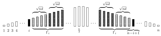
Figure 1: $\Gamma_{i}$ consists of the $2\sqrt{nd}$ positions following position $i$ and preceding the $i$-th last position, which is $n-i+1$. We estimate the probability that (1&2) none of the elements drawn with horizontal lines gets a huge noise added to it and (3) at least one of the elements drawn in crosshatch gets a huge noise and becomes a scan maximum.

Fix any $i\leq\frac{n}{2}-2\sqrt{nd}$. Figure 1 shows $\Gamma_{i}$ and illustrates the event whose probability we want to estimate now. Remember that $\nu_{i}$ denotes the additive noise at position $i$. Assume the following holds:

1. $\nu_{i+1},\ldots,\nu_{i+\sqrt{nd}}\leq d-\sqrt{\frac{d}{n}}$.

2. $\nu_{n-i},\nu_{n-i-1},\ldots,\nu_{n-i-\sqrt{nd}+1}\leq d-\sqrt{\frac{d}{n}}$.

3. There exist $j,j^{\prime}\in\Gamma_{i}$ such that $\nu_{j},\nu_{j^{\prime}}>d-\sqrt{\frac{d}{n}}$.

Choose $j$ to be minimal and $j^{\prime}$ to be maximal. Then $j>i+\sqrt{nd}$ and $j^{\prime}\leq n-i-\sqrt{nd}$. If the three properties above are fulfilled, then, by the choice of $j$ and $j^{\prime}$, $\overline{s}_{j}>\overline{s}_{i}$ for all $i<j$ and $i>j^{\prime}$: For $i\in\Gamma_{i}$, this follows from the minimality of $j$, the maximality of $j^{\prime}$. For $i\notin\Gamma$, $i\leq n/2$, we have $\overline{s}_{i}=\frac{i}{n}+\nu_{i}\leq\frac{i}{n}+d=\frac{i+\sqrt{nd}}{n}+d-\sqrt{\frac{d}{n}}\leq\overline{s}_{j}$ by the fact that $\nu_{j}>d-\sqrt{\frac{d}{n}}$.

Furthermore, $j$ or $j^{\prime}$ is a left-to-right maximum: Suppose not, then there must exist an $i<j$ or an $i>j^{\prime}$ that becomes a pivot which causes positions $j$ and/or $j^{\prime}$ to vanish. This, however, contradicts the property as shown above. Thus, if the three properties are fulfilled, we have a left-to-right maximum in $\Gamma_{i}$.

Let us estimate the probability that this happens. We have

$$\mathbb{P}\left(\nu_{i+1},\ldots,\nu_{i+\sqrt{nd}}\leq d-\sqrt{\frac{d}{n}}\right)=\left(\frac{d-\sqrt{d/n}}{d}\right)^{\sqrt{nd}}=\left(1-\frac{1}{\sqrt{nd}}\right)^{\sqrt{nd}}\geq\frac{1}{4}$$

if $\sqrt{nd}\geq 2$. The latter is fulfilled if $d\geq 4/n$. If $d=c/n$ is smaller, we easily get a lower bound of $\Omega(n)$ by restricting the adversary to the interval $[0,c/4]$: We can apply the bound for $d=4/n$ by scaling.

By symmetry, also

$$\mathbb{P}\left(\nu_{n-i},\ldots,\nu_{n-i-\sqrt{nd}+1}\leq d-\sqrt{\frac{d}{n}}\right)\geq\frac{1}{4}$$

Furthermore,

$$\mathbb{P}\left(\exists j\in\{i+\sqrt{nd}+1,\ldots,i+2\sqrt{nd}\}:\nu_{j}>d-\frac{d}{n}\right)=1-\left(\frac{d-\sqrt{d/n}}{d}\right)^{\sqrt{nd}}\geq 1-\frac{1}{e},$$

and the same lower bound holds for the probability that there exists a $j^{\prime}\in\Gamma_{i}$ as described above. Overall, the probability that $j$ and $j^{\prime}$ exist is constant, which proves the lower bound of $\Omega\bigl{(}\sqrt{n/d}\bigr{)}$.

To finish the proof, let us prove that, on average, we expect to see $\Omega(\log n)$ scan maxima. To do this, let us consider the sequence $s=(0,0,\ldots,0)$. We obtain $\overline{s}$ by adding noise from $[0,d]$. The ordering of the elements in $\overline{s}$ is now a uniformly distributed random permutation. We take a different view on the maximum-of-two pivot rule: We take $s_{1}$, get a half point for it and eliminate all elements smaller than $s_{1}$. If $s_{n}$ has also been eliminated, then we have completed this iteration. Otherwise, we take $s_{n}$, get another half point and again eliminate all smaller elements.

The number of scan maxima of $\overline{s}$ is at least the number of points we get. Since the elements of $\overline{s}$ appear in random order, the expected number of points is $\frac{1}{2}\cdot H_{n}$, where $H_{n}$ is the average-case number of left-to-right maxima. ∎

Now we turn to the upper bound for scan maxima.

Lemma 4.3.

For all sequences $s$ and $d\geq\frac{1}{n}$, we have

$$\mathbb{E}\bigl{(}\operatorname{min2-scan}_{d}(s)\bigr{)}\in O\left(\sqrt{\frac{n}{d}}+\log n\right).$$

Proof.

First, we observe that a necessary condition for an element $\overline{s}_{i}$ to become a pivot element is that it is either a left-to-right maximum (according to the usual rule), i.e., no element $\overline{s}_{j}$ for $j<i$ is greater than $\overline{s}_{i}$, or that it is a right-to-left maximum, i.e., no element $\overline{s}_{j}$ for $j>i$ is greater than $\overline{s}_{i}$.

Hence, an upper bound for $\operatorname{min2-scan}(\overline{s})$ is $\operatorname{c-scan}(\overline{s})$ plus the number of right-to-left maxima. The former is at most $O\bigl{(}\sqrt{n/d}+\log n\bigr{)}$, the latter can be analyzed in exactly the same way. Thus, the lemma follows. ∎

From Lemmas 4.1, 4.2, and 4.3 we immediately get tight bounds for the number of scan maxima with median-of-three rule.

Theorem 4.4.

For every $d\geq 1/n$, we have

$$\max_{s\in[0,1]^{n}}\mathbb{E}\bigl{(}\operatorname{m3-scan}_{d}(s)\bigr{)}\in\Theta\left(\sqrt{\frac{n}{d}}+\log n\right).$$

5 Quicksort and Hoare’s Find with Median-of-three Rule

Now we use our results about scan maxima from the previous section to prove lower bounds for the number of comparisons that quicksort and Hoare’s find need using the median-of-three pivot rule. We only prove lower bounds here since they match already the upper bounds for the classic pivot rule. We strongly believe that the median-of-three rule does not yield worse bounds than the classic rule and, hence, that our bounds are tight. Our main goal of this section is to prove the following result for Hoare’s find. This bound carries then over to quicksort.

Theorem 5.1.

For $d\geq 1/n$, we have

$$\max_{s\in[0,1]^{n}}\mathbb{E}\bigl{(}\operatorname{m3-find}_{d}(s)\bigr{)}\in\Omega\bigl{(}\textstyle\frac{n}{d+1}\sqrt{n/d}+n\bigr{)}.$$

Proof.

We use the maximum-of-two rule to prove this lower bound. To this end, consider the following sequence: Let $\Delta=\{1,\ldots,\frac{n}{3}\}\cup\{\frac{2n}{3}+1,\ldots,n\}$ and let $s$ be defined by

$$s_{i}=\begin{cases}\min(\frac{i}{n},\frac{n-1-i}{n})&\text{if $i\in\Delta$ and}\\ 1&\text{otherwise.}\end{cases}$$

Figure 2 gives an intuition how $s$ looks like. We observe that $s_{\Delta}$ is, up to scaling, identical to the sequence used in Lemma 4.2 (up to scaling). To analyze the number of comparisons, we distinguish between small and large values of $d$.

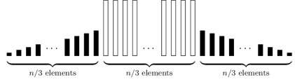
Figure 2: How the sequence of Lemma 5.1 looks like. The black elements contribute scan maxima, the white elements are large elements. All black scan maxima have to be compared to all or at least $\Omega(n/d)$ white elements.

First, assume that $d\leq\frac{2}{3}$. Then all elements of $\overline{s}_{[n]-\Delta}$ are greater than all elements of $\overline{s}_{\Delta}$, including the scan maxima of $\overline{s}_{\Delta}$. From Lemma 4.1 and the proof of Lemma 4.2, we know that $\overline{s}_{\Delta}$ contains $\Omega\bigl{(}\sqrt{n/d}+\log n\bigr{)}$ scan maxima. Each of these maxima has to be compared to all of the $n/3$ elements of $\overline{s}_{[n]-\Delta}$, resulting in $\Omega\bigl{(}n\cdot\bigl{(}\sqrt{n/d}+\log n\bigr{)}\bigr{)}$ comparisons.

The second case is $d\geq\frac{2}{3}$. Again, there are $\Omega\bigl{(}\sqrt{n/d}+\log n\bigr{)}$ scan maxima under the maximum-of-two rule in $\overline{s}_{\Delta}$, which carry over to $\overline{s}$. According to Lemma 4.1, there are at least that many median-of-three scan maxima (m3 maxima) in $\overline{s}$, but since $d$ may be greater than $\frac{2}{3}$, some of the m3 maxima may be from $\overline{s}_{[n]\setminus\Delta}$. This poses no harm because the position of the pivots is of no relevance to the sorting process, but only their magnitude. In turn, the magnitude of an m3 maximum is at most the magnitude of the corresponding maximum-of-two scan maximum (max2 maximum).

We can now bound the number of comparisons appropriately. The probability that an element $\overline{s}_{i}$ ($i\in[n]\setminus\Delta$) is greater than the first $\Omega\left(\sqrt{n/d}+\log n\right)$ m3 maxima is at least the probability that it is greater than all elements of $\overline{s}_{\Delta}$ maxima, which are located in $\overline{s}_{\Delta}$, i.e.

$$\mathbb{P}\left(\overline{\tau}_{i}>\text{ first }\Omega\left(\sqrt{n/d}+\log n\right)\text{ m3-LTRMs }\right)\geq\mathbb{P}\left(1+\nu_{i}>\frac{1}{3}+d\right)=\frac{2}{3d}.$$

Thus, by linearity of expectation, an expected number of $\Omega(n/d)$ elements of $\overline{s}_{[n]\setminus\Delta}$ are greater than the first $\Omega\bigl{(}\sqrt{n/d}+\log n\bigr{)}$ m3 maxima and have to be compared to all of them. This requires $\Omega\bigl{(}\frac{n}{d}\cdot\sqrt{\frac{n}{d}}\bigr{)}$ comparisons. Since we always need at least $\Omega(n)$ comparisons, the theorem follows. ∎

Since the number of comparisons that Hoare’s find needs is a lower bound for the number of quicksort comparisons, we immediately get the following result for quicksort.

Corollary 5.2.

For $d\geq 1/n$, we have

$$\max_{s\in[0,1]^{n}}\mathbb{E}\bigl{(}\operatorname{m3-sort}_{d}(s)\bigr{)}\in\Theta\bigl{(}\textstyle\frac{n}{d+1}\sqrt{n/d}+n\log n\bigr{)}.$$

Proof.

The result follows from Theorem 5.1 and the observation that quicksort always requires at least $\Omega(n\log n)$ comparisons. ∎

6 Hoare’s Find Under Partial Permutations

To complement our findings about Hoare’s find, we analyze the number of comparisons subject to partial permutations. For this model, we already have an upper bound of $O(\frac{n}{p}\log n)$, since that bound has been proved for quicksort by Banderier et al. [2].

We show that this is asymptotically tight (up to factors depending only on $p$) by proving that Hoare’s find needs a smoothed number of $\Omega\bigl{(}(1-p)\frac{n}{p}\cdot\log n\bigr{)}$ comparisons.

The main idea behind the proof of the following theorem is as follows: We aim at finding the median. The first few elements are close to and smaller than the median (few means roughly $\Theta((m/p)^{1/4})$). Thus, it is unlikely that one of them is permuted further to the left. This implies that all unmarked of the first few elements become pivot elements. Then we observe that they have to be compared to many of the $\Omega(n)$ elements larger than the median, which yields our lower bound.

Theorem 6.1.

Let $p\in(0,1)$ be a constant. There exist sequences $s$ of length $n$ such that under partial permutations we have

$$\mathbb{E}\bigl{(}\operatorname{c-find}_{p}(s)\bigr{)}\in\Omega\left((1-p)\cdot\frac{n}{p}\cdot\log n\right).$$

Proof.

For simplicity, we restrict ourselves to odd $n$ and permutations of $-m,-m+1,\ldots,m$ for $2m+1=n$. This means that $0$ is the median of the sequence. Let $Q=(m/p)^{1/4}$. We consider the sequence

$$s=(-Q,-Q+1,\ldots,-1,-m,\ldots,-Q-1,1,\ldots,m,0).$$

The important part of $s$ are the first $Q$ elements. All other elements can as well be in any other order.

Assume that the unperturbed element $\overline{s}_{i}=-Q+i-1$ ($i\leq Q$) becomes a pivot and is unmarked. The latter happens with a probability of $1-p$. The former means that all marked elements among $-Q+i,\ldots,-1$ are permuted further to the right (more precisely: not to the left of position $i$). Let

$$M_{i}=\min\bigl{(}\{\overline{s}_{j}\mid\overline{s}_{j}\geq 0,j<i\}\cup\{m+1\}\bigr{)}.$$

Then $\overline{s}_{i}$ contributes $M_{i}$ comparisons. (Actually, at least $M_{i}+Q-i$ comparisons, but we ignore the $Q-i$ since it does not contribute to the asymptotics.) Let $E_{i}^{k}$ be the event that the $i$-th position is unmarked, $\overline{s}_{i}=s_{i}$ becomes a pivot, and $M_{i}\geq k$. Using lower bounds for $\mathbb{P}\bigl{(}E_{i}^{k}\bigr{)}$, we get a lower bound for the expected number of comparisons.

Let $A$ be the number of marked positions prior to $i$, let $B$ be the number of marked elements among $-Q+i,\ldots,-1$ and among $0,\ldots,k$, and let $N$ be the total number of marked elements.

Given this and $A\leq B$, the probability of $E_{i}^{k}$ is

$$W_{k} =(1-p)\cdot\frac{N-A}{N}\cdot\frac{N-A-1}{N-1}\cdot\ldots\cdot\frac{N-A-B+1}{N-B-1}$$

$$\geq(1-p)\cdot\left(\frac{N-A-B}{N}\right)^{A}=(1-p)\cdot\exp\left(A\cdot\ln\left(1-\frac{A+B}{N}\right)\right)$$

$$\geq(1-p)\cdot\exp\left(-\frac{2A(A+B)}{N}\right)\geq(1-p)\cdot\exp\left(-\frac{4AB}{N}\right).$$

The first inequality holds since $A\leq B$ and therefore most factors cancel each other out. The second inequality holds since $\ln(1-x)\geq-2x$ for $x\in[0,\frac{3}{4}]$. The third inequality holds again since $A\leq B$.

This bound is monotonically decreasing in $A$ and $B$, and monotonically increasing in $N$. Thus, we need upper bounds for $A$ and $B$ and a lower bound for $N$. Now let $1/p\leq i\leq Q-1/p$, and let $k\geq\sqrt{m/p}$. At most $2pi$ positions prior to $i$, at most $2p(Q-i)$ positions after $i$ and before $Q$ are marked with a probability of $\Omega(1)$. Furthermore, at least $\frac{p}{2}n$ positions overall are marked, and at most $2pk$ elements among $0,\ldots,k$ are marked. The last two requirements happen with a probability close to $1$. This yields $A\leq 2pi$, $B\leq 2pk+2p(Q-i)\leq 3pk$ as well as $N\geq\frac{p}{2}n$. Since $i\geq 1/p$ and $Q-i\geq 1/p$, the probability that all these bounds are satisfied is at least a constant $c>0$. This allows us to bound $W$ as follows:

$$W_{k}\geq c\cdot(1-p)\cdot\exp\left(-\frac{48pki}{n}\right).$$

Let $K_{i}=\exp\bigl{(}-\frac{48pi}{n}\bigr{)}$. We observe that $K_{i}^{\sqrt{m/p}}\geq c^{\prime}\in\Omega(1)$. Using this to bound the expected number of comparisons, we get that the expected number of comparisons with the unmarked $\overline{s}_{i}$ as the pivot element is at least

$$W_{\sqrt{m/p}}\cdot\sqrt{\frac{m}{p}}+\sum_{k>\sqrt{m/p}}^{m}W_{k} \geq cc^{\prime}\cdot(1-p)\cdot\sum_{k=1}^{m}K_{i}^{k}=cc^{\prime}\cdot(1-p)\cdot K_{i}\cdot\frac{1-K_{i}^{m+1}}{1-K_{i}}$$

$$\geq\frac{cc^{\prime}}{2}\cdot(1-p)\cdot\frac{1}{1-K_{i}}\geq\frac{cc^{\prime}}{2}\cdot(1-p)\cdot\frac{n}{96pi}.$$

We use the linearity of expectation, sum over all $i\in\{1,\ldots,(m/p)^{1/4}\}$, and get the desired bound. ∎

For completeness, to conclude this section, and as a contrast to Sections 2 and 3, let us remark that for partial permutations, finding the maximum using Hoare’s find seems actually to be easier than finding the median: The lower bound constructed above for finding the median needed that there are elements on either side of the element we aim for. If we aim at finding the maximum, all elements are on the same side of the target element. In fact, we believe that for finding the maximum, an expected number of $O(f(p)\cdot n)$ for some function $f$ depending on $p$ suffices.

7 Concluding Remarks

We have shown tight bounds for the smoothed number of comparisons for Hoare’s find under additive noise and under partial permutations. Somewhat surprisingly, it turned out that, under additive noise, Hoare’s find needs (asymptotically) more comparisons for finding the maximum than for finding the median. Furthermore, we analyzed quicksort and Hoare’s find with the median-of-three pivot rule, and we proved that median-of-three does not yield an asymptotically better bound. Let us remark that also the lower bounds for left-to-right maxima as well as for the height of binary search trees [11] can be transferred to median-of-three. The bounds remain equal in terms of the number $n$ of elements.

A natural question regarding additive noise is what happens when the noise is drawn according to an arbitrary distribution rather than the uniform distribution. Some first results on this for left-to-right maxima were obtained by Damerow et al. [4]. We conjecture the following: If the adversary is allowed to specify a density function bounded by $\phi$, then all upper bounds still hold with $d=1/\phi$ (the maximum density of the uniform distribution on $[0,d]$ is $1/d$). However, as Manthey and Tantau point out [12], a direct transfer of the results for uniform noise to arbitrary noise might be difficult.

References

- [1] Alfred V. Aho, John E. Hopcroft, and Jeffrey D. Ullman. The Design and Analysis of Computer Algorithms. Addison-Wesley, 1974.
- [2] Cyril Banderier, René Beier, and Kurt Mehlhorn. Smoothed analysis of three combinatorial problems. In Branislav Rovan and Peter Vojtás, editors, Proc. of the 28th Int. Symp. on Mathematical Foundations of Computer Science (MFCS), volume 2747 of Lecture Notes in Computer Science, pages 198–207. Springer, 2003.
- [3] Daniel Cederman and Philippas Tsigas. A practical quicksort algorithm for graphics processors. In Dan Halperin and Kurt Mehlhorn, editors, Proc. of the 16th Ann. European Symp. on Algorithms (ESA), volume 5193, pages 246–258, 2008.
- [4] Valentina Damerow, Friedhelm Meyer auf der Heide, Harald Räcke, Christian Scheideler, and Christian Sohler. Smoothed motion complexity. In Giuseppe Di Battista and Uri Zwick, editors, Proc. of the 11th Ann. European Symp. on Algorithms (ESA), volume 2832 of Lecture Notes in Computer Science, pages 161–171. Springer, 2003.
- [5] Hannu Erkiö. The worst case permutation for median-of-three quicksort. The Computer Journal, 27(3):276–277, 1984.
- [6] C. A. R. Hoare. Algorithm 64: Quicksort. Communications of the ACM, 4(7):322, 1961.
- [7] C. A. R. Hoare. Algorithm 65: Find. Communications of the ACM, 4(7):321–322, 1961.
- [8] Peter Kirschenhofer and Helmut Prodinger. Comparisons in Hoare’s find algorithm. Combinatorics, Probability and Computing, 7(1):111–120, 1998.
- [9] Peter Kirschenhofer, Helmut Prodinger, and Conrado Martinez. Analysis of Hoare’s find algorithm with median-of-three partition. Random Structures and Algorithms, 10(1-2):143–156, 1997.
- [10] Donald E. Knuth. Sorting and Searching, volume 3 of The Art of Computer Programming. Addison-Wesley, 2nd edition, 1998.
- [11] Bodo Manthey and Rüdiger Reischuk. Smoothed analysis of binary search trees. Theoretical Computer Science, 378(3):292–315, 2007.
- [12] Bodo Manthey and Till Tantau. Smoothed analysis of binary search trees and quicksort under additive noise. In Edward Ochmański and Jerzy Tyszkiewicz, editors, Proc. of the 33rd Int. Symp. on Mathematical Foundations of Computer Science (MFCS), volume 5162 of Lecture Notes in Computer Science, pages 467–478. Springer, 2008.
- [13] Michael Mitzenmacher and Eli Upfal. Probability and Computing: Randomized Algorithms and Probabilistic Analysis. Cambridge University Press, 2005.
- [14] Douglas C. Schmidt. qsort.c. C standard library stdlib within glibc 2.7, available at http://ftp.gnu.org/gnu/glibc/, 2007.
- [15] Robert Sedgewick. The analysis of quicksort programs. Acta Informatica, 7(4):327–355, 1977.
- [16] Robert Sedgewick. Implementing quicksort programs. Communications of the ACM, 21(10):847–857, 1978.
- [17] Richard C. Singleton. Algorithm 347: An efficient algorithm for sorting with minimal storage. Communications of the ACM, 12(3):185–186, 1969.
- [18] Daniel A. Spielman and Shang-Hua Teng. Smoothed analysis of algorithms: Why the simplex algorithm usually takes polynomial time. Journal of the ACM, 51(3):385–463, 2004.
- [19] Daniel A. Spielman and Shang-Hua Teng. Smoothed analysis of algorithms and heuristics: Progress and open questions. In Luis M. Pardo, Allan Pinkus, Endre Süli, and Michael J. Todd, editors, Foundations of Computational Mathematics, Santander 2005, pages 274–342. Cambridge University Press, 2006.