Near-IR Integral Field Spectroscopy study of the Star Formation and AGN of the LIRG NGC 5135

Abstract

We present a study of the central $\rm 2.3\,kpc$ of NGC 5135, a nearby Luminous Infrared Galaxy (LIRG) with an AGN and circumnuclear starburst. Our main results are based on intermediate spectral resolution ($\rm\sim 3000$-$4000$) near infrared data taken with the SINFONI integral field spectrograph at the ESO VLT. The ionization of the different phases of the interstellar gas and the complex structures of the star formation have been mapped. Individual regions of interest have been identified and studied in detail.

For the first time in this galaxy, we have detected the presence of a high excitation ionization cone centered on the AGN by using the [SiVI]${\rm\lambda 1.96\,\mu m}$ line. So far, this structure is the largest reported in the literature for this coronal line, extending (in projection) as far as $\rm\sim 600\,pc$ from the galaxy nucleus. In a complex spatial distribution, a variety of mechanisms are driving the gas ionization, including SNe remnant shocks, young stars and AGN photoionization. The excitation of the molecular gas, however, is mainly produced by X-rays and SNe remnant shocks. UV-mechanisms like fluorescence represent a marginal overall contribution to this process, contrary to the expectations we might have for a galaxy with a recent and strong star formation. Our SNe rate estimations from [FeII]${\rm\lambda 1.64\,\mu m}$ are in excellent agreement with 6 cm radio emission predictions. Typical SNe rates between $0.01$-$\rm 0.04\,yr^{-1}$ were found for individual $\approx$ 200 pc-scale regions, with an overall SNe rate of $0.4$-$\rm 0.5\,yr^{-1}$. Even though NGC 5135 has suffered a recent starburst ($6$-$\rm 7\,Myr$ ago), the data strongly suggest the presence of a second, older stellar population dominated by red giant/supergiant stars. However, simple stellar population models cannot sharply discriminate between the different populations.

1. Introduction

Since their discovery (Kleinmann & Low 1970, Rieke & Low 1972), the importance of low-$z$ Luminous ($10^{11}L_{\odot}\leq L_{IR}\leq 10^{12}L_{\odot}$, LIRG) and Ultraluminous ($L_{IR}\geq 10^{12}L_{\odot}$, ULIRG) Infrared Galaxies has been widely recognized. (U)LIRGs are gas rich galaxies (Solomon et al. 1997), where an active nucleus and powerful starbursts coexist and contribute to the energy output (e.g. Genzel et al. 1998, Spoon et al. 2007). While LIRGs appear to be mostly spirals (Arribas et al. 2004, Alonso-Herrero et al. 2006a), ULIRGs are strongly interacting systems and mergers (e.g. Bushouse et al. 2002) evolving into intermediate-mass ellipticals (e.g. Genzel et al. 2001, Dasyra et al. 2006). Local (U)LIRGs have been proposed as possible counterparts of the submillimeter population observed at higher redshifts (Blain et al. 2002 for a review, see also Chapman et al. 2003, Frayer et al. 2003, Egami et al. 2004). Also, cosmological surveys with $Spitzer$ have shown that the majority of IR selected galaxies at $z\leq 1$ are in the LIRG class, while LIRGs and ULIRGs make a significant contribution to the IR galaxy population and to the star formation at $1<z<2$ and $z\geq 2$, respectively (Egami et al. 2004; Le Floch et al. 2004, 2005; Pérez-González et al. 2005; Caputi et al. 2007).

Detailed investigations of the physical properties, stellar populations, AGN-starburst connection and gas flows on these complex systems can only be obtained through integral field spectroscopy (IFS). Initial studies of small samples of (U)LIRGs based on 4-meter class telescope optical IFS have already been obtained (e.g. Colina et al. 2005, Monreal-Ibero et al. 2006, Alonso-Herrero et al. 2009). To extend these studies to larger samples, and also to the near-IR, we have started a survey of low-$z$ (U)LIRGs using state-of-the-art IFS like VLT/VIMOS (Arribas et al. 2008) and VLT/SINFONI (visual and near-IR, respectively). This survey (SIRIUS: Survey of luminous IR galaxies with Integral field UnitS) will allow us to characterize the kpc-scale ionization and kinematics of a representative sample of low-$z$ (U)LIRGs covering a wide luminosity range, several morphologies from spirals to interacting and advanced mergers, as well as different classes of activity. This will also form a local reference for future IFS studies of high-$z$ IR galaxies with instruments such as the Near-IR Spectrograph (NIRSpec) and Mid-IR Instrument (MIRI) on board of the James Webb Space Telescope (Gardner et al. 2006).

As part of our survey, we present our first results with SINFONI showing the power of near-IR integral field spectroscopy by studying the local LIRG NGC 5135. This is an SBab galaxy at $z=0.01396$ (from NED, at $\rm\approx 58.7\,Mpc$ assuming $H_{0}=70\,\rm km\,s^{-1}\,Mpc^{-1}$) which belongs to a group of seven galaxies (Kollatschny & Fricke 1989). Its dual nature as a starburst hosting an AGN and its almost face-on sky orientation make NGC 5135 an ideal prototype-object for detailed studies of these hybrid systems.

The first attempts to study NGC 5135 was made 25 years ago by Huchra(1983), Huchra et al. (1983) and Phillips et al. (1983), who classified this object as a Seyfert 2. A year later, Thuan (1984) found that this galaxy is also a bright UV source, with mixed Seyfert and starburst spectral characteristics (see also Kinney et al. 1993). Ulvestad & Wilson (1989) observed NGC 5135 at 6 and 20 cm using the VLA, as part of a larger sample of nearby Seyfert galaxies. An important diffuse radio component was measured in this morphologically asymmetric object, which is in turn aligned with the extended H$\alpha$ emission (Haniff et al. 1988, García Barreto et al. 1996). Because of the lack of an accurate optical nucleus, Ulvestad & Wilson chose the brightest radio source as the reference for the central region.

Almost 10 years later, González Delgado et al. (1998) published a study based on $Hubble$ $Space$ $Telescope$ ($HST$ from now on) and ground-based UV/optical imaging and spectroscopy to study possible starburst-AGN connections. They found independent pieces of evidence pointing towards the presence of a dusty, compact and powerful starburst in the central region (inner $\rm 2^{\prime\prime}$) of NGC 5135, which dominates the UV spectrum. From spectral modeling and colors, these authors estimated an age of between $3$ and $\rm 6\,Myr$ for the last starburst episode. They also concluded that the warm interstellar gas is outflowing, most likely because of the starbursts. In the optical, these authors detected a nuclear bar for this galaxy, which had been previously found in the near infrared (hereafter NIR) by Mulchaey et al. (1997).

Using Chandra X-ray observations, Levenson et al. (2004) revisited NGC 5135. Two strong central sources were detected and the (AGN) nucleus was correctly identified for the first time, showing that its important internal extinction had made it difficult to recognize in previous works. They highlighted the importance of the stellar processes even in X-rays, showing that almost all the soft emission ($0.4$-$\rm 1\,keV$) has a stellar origin, even nearby the AGN. Only the hard emission ($4$-$\rm 10\,keV$) is dominated by the active nucleus.

Alonso-Herrero et al. (2006a,b) and Díaz-Santos et al. (2008) studied this object as part of a sample of $\sim 30$ local LIRGs. With high resolution mid and NIR images (Gemini, $HST$) in different bands, they identified the individual H ii knots which are hidden at shorter wavelengths. In NGC 5135, compact Pa$\alpha$ emission ($\sim 1$-$\rm 2\,kpc$) from star formation was detected as well as a strong, nuclear warm dust component in the N-band.

The NGC 5135 SINFONI data allowed us to address some of the issues described above, as well as to show the scientific potential of our SINFONI data set. On the other hand, issues such as the general role of (U)LIRGs in galaxy formation and evolution will be better addressed with our entire sample in future papers of the series. We leave for the following paper of the series (hereafter, Paper II) a detailed kinematical study and mass estimation for this galaxy.

The paper is organized as follows: in Sec. 2 the observations (2.1), data reduction (2.2) and analysis (2.3) are described. Also, several maps are presented (2.4) and specific regions of study are identified (2.5). In Sec. 3 the main results and discussion are shown, including a study of the central gas and stellar structure (3.1), internal extinction structure (3.2), gas ionization mechanisms and young stellar population age (3.3), further characterization of the stellar population ages by using stellar absorption features (3.4), the H₂ excitation mechanisms (3.5) and estimations of the supernova rate (3.6). Finally, in Sec. 4 we present the conclusions.

2. Observations and Data Reduction

2.1. Observing with SINFONI

The observations were carried out in service mode with SINFONI (Eisenhauer et al. 2003, Bonnet et al. 2004), the NIR integral field spectrometer mounted at VLT-Yepun (Cerro Paranal, Chile), with no AO-assisted guiding. The galaxy was observed separately in the H ($\rm 1.45-1.85\mu m$ ) and K ($\rm 1.95-2.45\mu m$) bands during April and May 2006. Observing the H and K-bands independently provides a higher spectral resolution ($\sim$ 3000 and $\sim 4000$, respectively) compared to the combined H+K band mode ($\rm\sim 1500$). The full-width-at-half-maximum (FWHM from now on) as measured from sky lines is $\sim 6\,\rm\AA$ for the H-band and about $\sim 5\,\rm\AA$ for K. The dispersions are $\rm 2$ and $\rm 2.5\,\AA\,pixel^{-1}$ for H and K, respectively. The $\rm 64\times 64$ spatial pixel (spaxels) field-of-view (FoV from now on) was centered close to the region where the AGN is located (Levenson et al. 2004). With a scale of $\rm 0.250^{\prime\prime}pixel^{-1}$, SINFONI provides a two-dimensional field of $\rm 8^{\prime\prime}\times 8^{\prime\prime}$.

For the H-band galaxy data, the total on-target integration time was 40 minutes (divided into 3 observation blocks, hereafter OBs), with an average seeing (FWHM of the point-spread-function, hereafter PSF) and airmass of $\rm 0.54^{\prime\prime}$ and 1.24, respectively. For the K-band data, the corresponding values were 25 minutes (2 OBs), $\rm 0.62^{\prime\prime}$ and 1.04 airmass. An entire K-band OB was discarded because of the high seeing ($\rm>2^{\prime\prime}$). Given the strong variations of the IR sky with time, the observing blocks were split into shorter on-source integrations of 150 seconds each. Between them, we obtained identical exposures of the sky background (ABBA pattern) by nodding the telescope to a point shifted $\Delta\alpha=42^{\prime\prime}$ and $\Delta\delta=87^{\prime\prime}$ from the galaxy nucleus. In this way, each “object integration” has a corresponding “sky integration” which was subtracted during the pipeline processing to remove (to first order) the sky signal from the final data cube. Also, the object and sky frames were jittered within a box width of $\rm 1.5^{\prime\prime}$ to get rid of detector effects (bad pixels).

2.2. Data Reduction

The basic data reduction was performed with the SINFONI Pipeline (version 1.8.2). Dark subtraction, flat-field normalisation, pixel linearity, geometrical distortion and wavelength calibration corrections were applied for each object-sky pair by using the products of SINFONI standard calibration plan. The calibration products (e. g. darks and flats) are generated on a daily basis, with the exception of the linearity and geometrical distortion data which are produced monthly. The wavelength calibration was performed with Xe-Ar and Ne lamps for the H and K-bands, respectively. The arc-frames include about 15 strong emission lines, well spread along the corresponding wavelength ranges. We double-checked the wavelength calibrations on the individual object-sky frames by tracing the position of about 10-15 strong sky-lines along the detector. For the H-band data, we found a systematic offset in wavelength of $\rm+1.6\pm 0.1\AA$, independent of the data frame used for the measurements. A similar situation affects the K-band data, where an offset of $\rm+2.3\pm 0.3\AA$ was found. Although these shifts are smaller than the spectral resolution ($\rm FWHM=5$-$\rm 6\AA$) they correspond to almost 1 pixel offset. Therefore, we decided to correct for them given their amplitude and systematic presence in the data. As a final check and after applying the offset corrections, we compared for several spaxels the measured and theoretical arc-line positions, repeating the measurements in different frames. From the distribution of their differences, we estimated the ($\rm 3\,\sigma$) uncertainty in the wavelength calibration to be $\leq 1.3$ and $\rm\leq 1\,\AA$ for the H- and K-band spectral ranges, respectively.

The background sky was subtracted for each individual $\rm 150\,s$ object exposure. The SINFONI Pipeline does not only subtract the object/sky pairs but it also applies other correction algorithms in order to minimise the sky line residuals. Despite the fact that the sky line relative positions of each object/sky pair were between spectral resolution limits, the sky frames were slightly shifted in wavelength with respect to their object pairs to reduce the P-Cygni-type residuals. In a second step, the pipeline includes an implementation of the sky subtraction package described by Davies et al. (2007). This code allows to separately scale different transitions of the telluric OH lines before sky subtraction. After the correction, the sky-subtracted object frames present very small sky-line residuals whose importance (in the worst cases) is purely cosmetic.

At this point, the signal (counts) from the object frames within an OB (between 5 and 6 on-target frames per OB) were combined to generate the integrated data-cubes for each band. Given the jittering applied during observations, the pipeline re-aligned the individual object frame centers before combination. As a test for these alignments, we generate a individual data-cubes from each object frame; the position of the three more prominent peaks in the continuum (for H and K-band) were traced by fitting two-dimensional elliptical Gaussians and the offsets were re-calculated. The data-cubes generated with the new offsets were in excellent agreement with the pipeline products. In fact, the majority of the offsets used by the pipeline were recovered by our method within a 10% uncertainty. Consequently, we decided to stick to the pipeline data-cube products, while our cube alignment method will be used in following steps of the reduction.

As part of the calibration plan, spectrophotometric standard stars were observed along with our target object in order to perform the flux calibration. For each of the three H-band OBs an early-type star was observed (Hip 075902, Hip 068496 and Hip 065630 of spectral types B9V, B7II and B3IV, respectively), while only one star was used for the two consecutive K-band OBs (Hip 078004, B3/B4V). The stellar spectra were extracted within an aperture of $\rm 6\,\sigma$ of the best two-dimensional Gaussian fit of the light profile (between $5$ and $6^{\prime\prime}$). The measured spectra were divided by a theoretical spectrum for the corresponding stellar type, generating a multiplicative “sensitivity function” to be applied to the object data. We use the models of Pickles (1998) as our theoretical templates after scaling them to the corresponding magnitudes listed in the Hipparcos catalogue (Perryman et al. 1997).

For the H-band stars, we found some differences between the three individual sensitivity functions. The corrections in the central range $\rm 1.52$-$\rm 1.75\,\mu m$ are in very good agreement between the three functions, showing relative deviations within 5%. In the extremes of the wavelength range ($\leq 1.50$ and $\rm\geq 1.75\,\mu m$), however, relative differences could be as large as 15%. This suggests that the main source of uncertainty is not coming from Pickles’ models (our “real” spectra) neither from peculiarities of the individual stars but from variations in the atmospheric transmission during observation (each star was observed just after one object OB, with airmass of 1.1, 1.3 and 1.5, respectively). We decided to apply the individual sensitivity functions to their corresponding OBs. Each of these functions has implicit the atmospheric transmission at a time and airmass close to that of the object observation. The results for the flux calibrated OB’s data were very good, with no strong residuals from transmission variations. In any case, because the only H-band line we will use is the [FeII]${\rm\lambda 1.64\,\mu m}$ (essentially in the center of the band), the effects of the correction in the extremes of the wavelength range are purely cosmetic.

One problem we found with Pickles’ models is that for many of our spectral types the models do not include particular stellar features in the NIR spectrum, but they just present a smooth continuum resembling that of a black body. If we do not take care of this, the spectral features of the star will show up in the galaxy spectrum. Fortunately, lines from the Brackett series in absorption are essentially the only spectral features we found in our stellar spectra. So they were modeled with Gaussians and the stellar spectra were normalised before flux calibration. The residuals from this process were negligible.

Once the OB’s spectra were reduced and flux calibrated, we combined the individual OBs in “final” data cubes for H- and K-bands. We estimated the offsets between OBs by finding the three main peaks in the continuum, as described above for the individual frame combination within an OB. As a final check, we compared our integrated fluxes in H and K with 2MASS data (Skrutskie et al. 2006). After adapting the spectral range to the $K_{s}$-band used in 2MASS, selecting a galaxy’s central region comparable to our FoV and taking into account zero-point considerations, we found a good agreement in fluxes within 10% uncertainty for both bands. This is consistent with our maximum error estimation (15%) found between individual OB’s flux calibrations in H. In Fig. 1 and 2 we present K- and H-band integrated spectra of six regions in NGC 5135 (see Fig. 3 and Secs. 2.5 and 3.1 for further details about the regions).

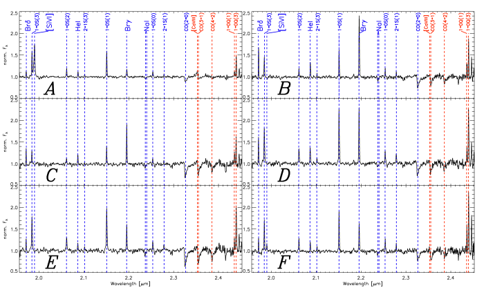
Figure 1.— Observed-frame, normalized K-band spectra of six selected regions in NGC 5135. The spectra were integrated within circular apertures of $\rm 0.62^{\prime\prime}$ diameter, corresponding to $\rm\approx 180\,pc$. Different emission lines and absorption bands are labeled. Blue labeled features are those used in this study.

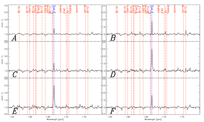
Figure 2.— Observed-frame, normalized H-band spectra of six selected regions in NGC 5135. The spectra were integrated within circular apertures of $\rm 0.54^{\prime\prime}$ diameter, corresponding to $\rm\approx 157\,pc$. Different emission lines and absorption bands are labeled. Blue labeled features are those used in this study.

2.3. Emission Line Fitting

The (redshifted) line peak, flux, equivalent-width (EW) and FWHM were calculated from many of the emission lines presented in H- and K-bands. Other parameters like galactocentric velocities and velocity dispersions will be presented and analysed in Paper II.

A single Gaussian component provides a good fit for the individual emission lines. We have used a nonlinear least-squares minimisation algorithm implemented in Image Data Language (hereafter, IDL) to perform the fitting. This method is comparable to other standard algorithms used for line fitting and implemented with other packages like IRAF. For each spaxel, local pseudocontinuum levels were calculated for each spectral feature. Two bands were defined at each side of the emission lines and linear fits were applied between their average flux values. In this way, our fitting algorithm weights each pixel with an error spectrum; it includes the Poisson noise, flux calibration uncertainties and errors in the local pseudocontinuum level.

After subtracting the pseudocontinuum, the fitting algorithm returns fluxes, EWs and FWHMs among other parameters (like the Gaussian $\sigma$ and peak position in $\rm\AA$) for all our lines.

A similar treatment was used for the stellar absorption features CO(2-0) (at $\rm 2.29\,\mu m$) and NaI (at $\rm\lambda 2.206-2.208\,\mu m$). Fluxes and EWs of the former were calculated by using the spectroscopic index definition of Kleinmann & Hall (1986). The NaI line features were measured by using the index definition from F$\ddot{o}$rster Schreiber (2000). In the bottom panels of Fig. 4 we present maps of the CO(2-0) feature; the weak NaI line is not suitable for mapping but for integrated region analysis only. Given the asymmetric shape of the CO(2-0) band and the doublet nature of the NaI absorption, we have not calculated FWHMs for these features. We will leave that for Paper II, where the use of stellar libraries and spectral synthesis methods will be applied to derive the stellar kinematics.

2.4. Flux, EW and FWHM Maps

In Fig. 3 we present maps for the different phases of the interstellar medium (hereafter ISM) including the emission gas lines Br$\gamma$ (at $\rm 2.17\,\mu m$), the H₂ transition 1-0 S(1) (at $\rm 2.12\,\mu m$), HeI$\rm\lambda 2.06\,\mu m$, [SiVI]$\rm\lambda 1.96\,\mu m$ and [FeII]${\rm\lambda 1.64\,\mu m}$, including fluxes (none are corrected for internal extinction, see Sec. 3.2), EWs and FWHMs (both in $\rm\AA)$. In a similar way, Fig. 4 shows the stellar components traced by H- and K-band continua and the CO (2-0) band at $\rm 2.29\,\mu m$ (both flux and EW). All maps are centered close to the nuclear peak of the K-band continuum. At the distance of NGC 5135, our $\rm 8^{\prime\prime}\times 8^{\prime\prime}$ FoV corresponds to the central $\rm 2.3\,kpc\times 2.3\,kpc$. The signal-to-noise (hereafter S/N) per $\rm\AA$ (per spaxel) is typically above 50 at the peaks of the emission, while in the diffuse regions it drops to about 20. The white areas on the maps (Fig. 3 and bottom panels of Fig. 4) donnot present enough signal for reliable detections in individual spaxels.

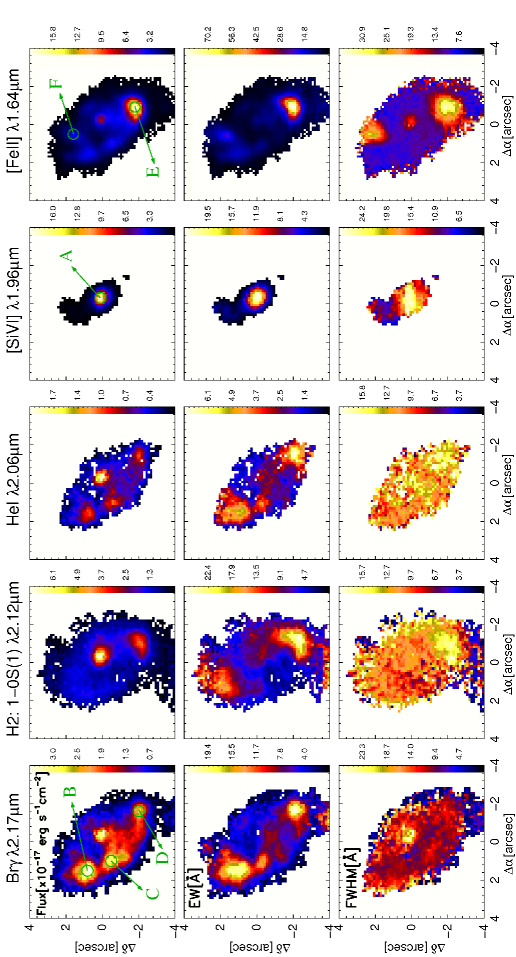
Figure 3.— Gas emission line maps of NGC 5135. White regions are those with unreliable detections for individual spaxels. From left to right: Br$\gamma$, H₂ (1-0 S(1) transition at $\rm 2.12\,\mu m$), HeI$\rm\lambda 2.06\,\mu m$ [SiVI]$\rm\lambda 1.96\,\mu m$ and [FeII]$\rm\lambda 1.64\,\mu m$. From top to bottom: fluxes (non-corrected for internal extinction), EW and FWHM. The angular size of the spatial pixels corresponds to $\rm 0.125\times 0.125\,arcsec^{2}$. The arrows in the flux maps show the location of our six selected regions A-F and the circles represent the selected aperture sizes. At the distance of NGC 5135, the $\rm 8^{\prime\prime}\times 8^{\prime\prime}$ FoV corresponds to the central $\rm 2.3\,kpc\times 2.3\,kpc$. In all panels, North is up and East is left.

2.5. Selected Regions for study: Integrated spectra

To better understand the processes taking place in the nucleus and neighbouring regions, we have chosen six separate regions for a more meticulous study. They have been labeled as A, B, C, D, E and F, and their locations are indicated in the first row of Fig. 3. We refer the reader to Sec. 3.1 for a detailed description of the reasons behind this selection. In Fig. 3, the circles’ diameters correspond to the seeing of the observations within which we integrate our spectra to improve our S/N ratio. Such a S/N enhancement makes it possible to run certain tests and models with weak emission features (e.g. NaI, 2-1 S(1)); this would be unfeasible on a spaxel-by-spaxel basis. At the distance of NGC 5135, we are integrating within aperture diameters of 157 pc in H-band and 180 pc in K-band.

To extract the integrated spectra, we have used the IDL routine APER, available in the IDL Astronomy Library. This task allowed us to obtain fluxes from circular apertures by polynomial interpolation of the squared pixels. Aperture uncertainties were also provided by this program by using a close neighbours technic. As we did for the data-cube individual spaxels, we run our Gaussian fitting program on these integrated spectra, obtaining fluxes, EWs, FWHMs and other parameters, this time including the aperture error as an extra source of uncertainty. In Table 7 we present fluxes, EWs, FWHMs and their $1\,\sigma$ errors for each of our spectral features corresponding to our six selected regions. In general, the flux uncertainties were between 10–20 %, although weak features (e.g. 2-1 S(3)) have larger uncertainties. Typically, the errors were dominated by Poisson uncertainties. However, for lines in the blue extreme of K-band (Br$\delta$, 1-0 S(3), [SiVI]) the flux calibration and pseudocontinuum level determination are more uncertain given the variability and lower transmission of this spectral region.

Finally, we performed internal flux extinction corrections for our measurements in regions A-F. Mean extinction values were applied for the corresponding aperture spaxels derived from the extinction map (see Fig. 6 and Sec. 3.2 for details). We present the corrected fluxes for all our lines in Table 7 with the mean $A_{V}$ extinction applied for each region. It is clear from the table that some of the uncertainties from the extinction corrections are relatively large compared to the uncorrected flux errors. In the extreme cases, the original $<$10% flux uncertainty of a strong line becomes an about 30% error in the corrected measurement. Therefore, we decided to use fully or non-corrected fluxes according to these criteria: Corrected fluxes were used when luminosities and other absolute flux dependant quantities (like hydrogen column densities, $N_{H}$) are calculated. Also, for the flux ratio [FeII]/Br$\gamma$ we make use of fully-corrected fluxes for both lines. Non-corrected fluxes were only used for flux-ratio plots between lines in the K-band.

The reason for the criteria described above is to minimise the uncertainties whenever possible. For the flux-ratio criteria, we found that the extinction correction between the bluest and reddest lines in K-band differs by 6-8% depending on the A-F regions. In a flux ratio, this uncertainty is negligible compared to the individual flux errors in both lines. Therefore, while we do not significantly improve our measured ratio, we increase our error bars by about a factor of 3. When [FeII]$\rm\lambda 1.64\,\mu m$ is involved, however, the situation is different. In a similar analysis, we found that the extinction correction between [FeII] and a K-band line can easily differ by more than 10%, even reaching 20% differences in the worst cases. These corrections are comparable to or larger than the errors of the non-corrected flux ratios. Therefore, when [FeII] flux is involved, internal extinction must be taken into account.

3. Results and Discussion

In this section we present the results and analysis of the spatially resolved spectroscopy of NGC 5135. The many spectral features detected provide a variety of tracers of different physical phenomena. The most frequently used emission lines in the present work include Br$\gamma$ ($\rm 2.16\,\mu m$, recent star formation tracer), the H₂ transition 1-0 S(1) ($\rm 2.12\,\mu m$, warm molecular gas), [SiVI] ($\rm 1.96\,\mu m$, an AGN tracer) and [FeII] ($\rm 1.64\,\mu m$, a supernova remnant tracer). Also, other features like the CO band at $\rm 2.29\,\mu m$, the NaI doublet at $\rm\lambda 2.206-2.208\,\mu m$, HeI$\rm\lambda 2.06\,\mu m$, Br$\delta$ and the H₂ transitions 1-0 S(0), 1-0 S(2), 1-0 S(3), 2-1 S(1) and 2-1 S(3) were used during the analysis.

3.1. Central Gas and Stellar Structure

It is evident from the Figs. 3 and 4 flux maps that they are tracing different structures within the central $\rm 2.3\,kpc$ of NGC 5135. In general, the number and spatial location of local flux peaks are totally different from one tracer to another. Only the nuclear region of this galaxy presents flux peaks in all maps. The EW maps (Fig. 3, second row and Fig. 4, bottom right panel) also differ substantially from tracer to tracer, showing local peaks usually matching those in flux. The only exceptions correspond to the nuclear region, where the AGN increases the continuum level (i. e. decreasing the EW values), and to the NE region of the H₂ map, where a EW peak does not have a flux peak counterpart. The FWHM maps (Fig. 3, third row) are rather smooth compared to the previous two. Only the FWHM([FeII]) map presents clear structure, with two local peaks (north and south) separated by a third one in the nucleus. More detailed descriptions of some maps will be presented in the following pages, while some other enlightening comparisons between them will be used in different sections of this paper.

As mentioned in Sec. 2.5, the chosen regions A to F will help us to understand the different processes affecting the gas and stars in this galaxy. However, they will also be useful to label some of the structural features observed in Fig. 3 flux maps. Therefore, a brief description of these regions follows. Region A corresponds to the nuclear peak in the K-band continuum. This region includes the AGN nucleus; all emission lines measured and the continuum have a peak at this location. Regions B, C and D correspond to bright peaks on the Br$\gamma$ flux map, where probably very recent star formation has taken place. Region E corresponds to the most prominent peak on the [FeII] flux map, presumably indicating the strong effects of shocks from supernova (SNe from now on). Also, this region matches the position of the secondary peak observed in the 1-0 S(1) transition of H₂. We remark that the peaks of regions D and E, despite being close ($0.56^{\prime\prime}$), are not coincident. In terms of their integrated spectra, D and E share only a few common flux spaxels (equivalent to 1-2 spaxel’s area) in the K-band ($0.62^{\prime\prime}$ aperture), while their H-band spectra are independent because of the smaller aperture used ($0.54^{\prime\prime}$). Any PSF-wing contamination effects were found to be negligible within these two apertures. Finally, region F corresponds to a local peak on both the [FeII] flux and FWHM maps. It is also coincident with an extended structure in [SiVI]. In Fig. 1 and 2 we show the extracted K and H-band spectra from these six regions.

3.1.1 Coronal Gas

The [SiVI]$\lambda 1.96\mu$m and [CaVIII]$\lambda 2.32\mu$m coronal lines are observed in the data, the former being our main AGN tracer (Fig. 3, fourth column; e.g. Maiolino et al. 2000, Rodríguez-Ardila et al. 2006a). The [CaVIII] line is too faint and too close to CO (3-1) to be measured reliably. The ionization potential required to produce the [SiVI] line (167 eV) is usually associated to Seyfert activity where the gas is excited just outside the broad line regions of AGNs.

As we can see in the Fig. 3 flux map, the [SiVI] line traces the galaxy nucleus and it also presents a weaker “plume” to the NE. This particular region, in terms of spatial scales, is at least $\rm 4\times$ larger ($\rm\approx 600\,pc$ in this case) than previous reports on different Seyfert galaxy samples (e.g. Prieto et al. 2005, Rodríguez-Ardila et al. 2006a) where [SiVI] structures have at the most $\rm\approx 150\,pc$ across. This finding, together with evidence for a similar structure to the SW (see Sec. 3.3.2), suggest that we have detected, for the first time, the presence of ionizing cones in NGC 5135. According to Rodríguez-Ardila et al. (2006a), the morphology of [SiVI] and other coronal gas is preferably aligned with the direction of the traditional lower-ionization cones (i. e. traced by [OIII]) seen in Seyfert galaxies.

3.1.2 Ionized Gas

The Br$\gamma$ and HeI maps (Fig. 3, first and third columns) show emission dominated by three extra-nuclear sources at $\approx 2^{\prime\prime}$ from the galaxy center, corresponding to regions B, C and D. As other recombination lines, the Br$\gamma$ feature is usually associated to recent star formation, where photoionization from massive young stars is taking place. The higher ionization energy of HeI (24.6 eV) compared to hydrogen (13.6 eV) makes it a good tracer of the most massive O-B stars and therefore, in principle, of the youngest populations in starforming regions. An unambiguous interpretation of the HeI line, however, is rather controversial. Different authors have claimed that this emission depends on the nebular density, temperature and dust content, apart from the He/H relative abundance and relative ionization fractions (Shields 1993, Doherty et al. 1995, Lumsden et al. 2001). Therefore, without detailed photoionization models, certain frequently used tests like the HeI/Br$\gamma$ ratio are very uncertain when analysing the hottest star temperature and tracing this population in H ii regions. This is why we will use HeI only as a first order spatial identification of the youngest stellar populations. The fluxes, EWs and FWHMs of this feature are included in Table 7 for completeness.

By comparing the Br$\gamma$ and HeI flux maps, it is evident that both are tracing the same structures, particularly the three extranuclear peaks mentioned above (B, C and D). It is worth noticing, however, that the strongest peak of the HeI-emission corresponds to the central region A, as it is also the case of Br$\gamma$ after extinction correction (see Table 7). These probably reflect that processes associated to the AGN (e.g. shocks, photoionization, X-ray emission) contribute to the observed fluxes. However, given the size of our aperture (180 pc), we cannot discard the contribution of very recent starburst to further ionize the AGN vicinity. González-Delgado et al. (1998) have shown for a small sample of local Seyfert 2 galaxies that, even in UV/optical wavelengths (highly affected by extinction), starforming knots are clearly identified at distances well below 100 pc from the nucleus (see also Cid Fernandes et al. 2004 and Davies et al. 2007).

¿From higher resolution (HST/NICMOS) Pa$\alpha$ maps (Alonso-Herrero et al. 2006a) we know that at least regions B and C have a much more complex structure than observed here, and are composed of a few individual knots of star formation. At least part of the important diffuse emission component observed in the Br$\gamma$ map presents some structure in the Pa$\alpha$ counterpart, particularly within the “triangle” formed by A, C and D.

3.1.3 Partially Ionized Gas

Different astronomical objects are capable of emitting [FeII]$\rm\lambda 1.64\,\mu m$, including H ii regions, SNe remnants (hereafter SNRs) and AGNs, meaning that this line can be excited by different processes (see Sec. 3.3 for details).

Strong [FeII]$\rm\lambda 1.64\,\mu m$ emission is produced by free electron collisions in hot gas ($10^{3}$-$\rm 10^{4}\,K$). Its low ionization energy (16.2 eV), however, indicates that this line is strong only in partially ionized regions; otherwise the Fe would be in higher ionization states. The SNR shocks are a suitable mechanism to produce partially ionized zones and therefore the [FeII] flux has been frequently used as a SNe rate indicator (e.g. Colina 1993, Alonso-Herrero et al. 2003, Labrie & Pritchet 2006, see Sec. 3.6 for more references; see also Vanzi et al. 1996 for a different view). It is possible, however, that X-ray photoionization (e.g. from AGN or binary stars) produces a similar effect to that of shocks in the surrounding gas (Maloney et al. 1996).

Our [FeII] flux map is the most complex in structure (Fig. 3, fifth column), where two strong and three weaker extranuclear peaks are observed. The most prominent one corresponds to our E region and it seems to be a hot spot for SNe explosions given its high FWHM ($\rm\approx 513\,km\,s^{-1}$). On the other hand, our region F is also associated to a high FWHM zone but without a particularly large [FeII] emission in comparison to the other extranuclear peaks. This region seems to match with the [SiVI] “plume” mentioned above. Developing more detailed kinematical arguments is beyond the scope of this paper and we will leave such analysis for Paper II. In Sec. 3.3.1 we will contrast the FeII with Br$\gamma$ fluxes to shed some light on the dominant mechanisms responsible for heating the gas in the different regions.

3.1.4 Warm Molecular Gas

The observed H₂ features in the spectra (Fig. 1) are formed by roto-vibrational transitions of the molecules. Different mechanisms have been proposed as external energy sources including UV-fluorescence, thermal collisional excitation by SNe fast shocks and X-rays.

Our strongest warm molecular gas tracer, 1-0 S(1), shows a very different structure than previous indicators (Fig. 3, second column). Two intensity peaks dominate the emission: the strongest at the nucleus and the weaker peaking in region E, matching the main peak in [FeII] flux. Both peaks are broad (the later, spatially resolved), but the one in E is the dynamically hotter as shown in the FWHM map. The remaining H₂ flux has a diffuse appearance at our spatial resolution.

3.1.5 Giant and Supergiant Stellar Component

In young starburst galaxies, massive ($\rm<40\,M_{\odot}$) red giants and supergiants with ages between 10-100 Myr dominate the integrated NIR continuum emission. As the population evolves with time, less massive giants start dominating the emission. Few Gyr later, the IR and bolometric luminosities are dominated by the low mass giants near the tip of the Red Giant Branch (Renzini & Buzzoni 1986, Chiosi et al. 1986, Origlia & Oliva 2000). Spectral features such as the CO bands at $2.29\,\mu$m and the NaI doublet (at $2.206$ and $2.208\,\mu$m) are typical of K and later stellar types and also trace the luminous red giant and supergiant populations. The bottom panels of Fig. 4 show the flux and EW of the CO$\lambda 2.29\,\mu$m band. White regions are those with unreliable detections of CO in individual spaxels.

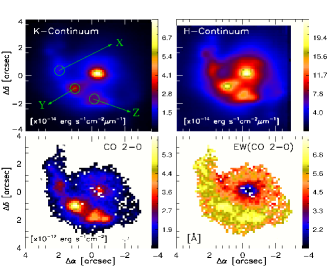
Figure 4.— Stellar emission traced by different indicators. White regions are those with unreliable measurements of CO in individual spaxels. Top panels: SINFONI K- and H-band continuum flux maps, the former indicating selected regions X, Y and Z. Bottom: Flux of CO (2-0) band at $\rm 2.29\,\mu m$ (left panel) and its EW (right panel). The angular size of the spatial pixels corresponds to $\rm 0.125\times 0.125\,arcsec^{2}$.

In Fig. 4 top panels, the H- and K-band continuum maps show a different spatial distribution than all previous emission line maps in Fig. 3. We observed three extra-nuclear peaks which donnot correspond to any of our A-F regions. However, from higher spatial resolution J-band continuum data (HST/NICMOS, Alonso-Herrero et al. 2006a) we know that these regions have a much more complex spatial structure with a series of knots. In any case, the strong diffuse emission component observed in their J-band continuum is also present in our SINFONI NIR data.

In general, from the four panels of Fig. 4 we see that all these indicators are essentially tracing the same structures, particularly in the extra-nuclear zone. The only exception occurs in the nuclear A region, where the strong NIR-continuum emission does not present a comparable counterpart in CO$\lambda 2.29\,\mu$m flux map.

In Sec. 3.4 we will go further on characterising the stellar population and its spatial structure by using these tracers. We will also estimate its age in different regions by using simple stellar population models (SSP models from now on).

3.1.6 Overall Picture

Summarising, all the structural components described in this section clearly show different spatial distributions through their associated spectral feature maps. We wish to highlight that, apart from region A and region E (the [FeII]-main-peak / H₂-secondary peak pair), many of the other line peaks are not spatially coincident with each other. We show this in Fig. 5. Three contour maps are overplotted including Br$\gamma$, [FeII] and K-band continuum, where the circles represent the position of the peaks for each map, having approximately the diameter of our extraction apertures. According to StarBurst99 models (hereafter SB99, Leitherer et al. 1999), these spectral features and K-band emission might be tracing stellar populations on different evolutionary stages, pointing towards ages of $\approx$ 6 Myr, $\leqslant$40 Myr (assuming a SNR origin of [FeII]-emission) and $\geqslant$200 Myr, respectively. In Secs. 3.3.1 and 3.4 we present a more detailed analysis of the stellar populations by using Br$\gamma$, the CO$\lambda 2.29\,\mu$m band, NaI$\lambda 2.21\mu$m and NIR-continuum. See also Secs. 3.3.1 and 3.6 for some discussion concerning the origin of [FeII]-emission in this galaxy.

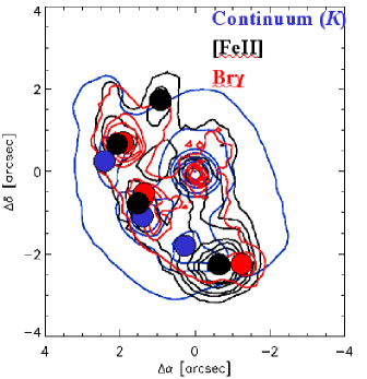
Figure 5.— Three contour maps overplotted: K-band continuum (blue), [FeII] (black) and Br$\gamma$ (red). In the same colors, local peaks of each map are marked by circles of approximately the same size than our extraction apertures.

3.2. Internal Extinction Map

Large amounts of dust and gas are usually found in local (U)LIRGs, hiding an important fraction of their star formation and AGN activity (Sanders et al. 1991, Sanders & Mirabel 1996, Solomon et al. 1997). Dust grains are mainly responsible for the absorption of UV/visual photons and re-emitting them as sub-millimeter and FIR radiation. In the NIR range, dust also absorbs and scatters radiation, but its effects are much smaller than at shorter wavelengths.

For NGC 5135, the effects of internal extinction become apparent in González Delgado et al. (1998) work. By comparing their optical (606W at $HST$/WFPC2, their Fig. 1) and UV-continuum maps ($HST$/FOC, their Figs. 5 and 6b) we found that our nuclear region A (centered at $+1.7^{\prime\prime}$N, $+0.4^{\prime\prime}$W in their coordinate system) almost disappear in the UV compared to visual, while starforming regions like E retain their morphologies in both wavelengths. This suggests that the AGN neighborhood is more obscured than other circumnuclear regions of this galaxy.

We can estimate the internal gas extinction in NGC 5135 by using observations of different hydrogen recombination lines. We adopt our own Br$\gamma$ and Br$\delta$ measurements for this purpose. The theoretical ratio between these two lines (Br$\gamma$/Br$\delta$ = 1.52 at $T=10\,000\,\rm K$ and $n_{e}=10^{4}\,\rm cm^{-3}$, Osterbrock 1989) was compared with the measured fluxes for each spaxel. Therefore the extinction in magnitudes ($A_{\lambda}$) for both lines can be combined in the form

$$A_{Br\gamma}-A_{Br\delta}=-2.5\cdot\Big{[}\log\Big{(}\frac{F_{Br\gamma,O}}{F_{Br\gamma,T}}\Big{)}-\log\Big{(}\frac{F_{Br\delta,O}}{F_{Br\delta,T}}\Big{)}\Big{]}$$

$$=-2.5\cdot\log\Big{[}\frac{(F_{Br\gamma}/F_{Br\delta})_{O}}{(F_{Br\gamma}/F_{Br\delta})_{T}}\Big{]}$$ (1)

where $F_{\lambda,O}$ and $F_{\lambda,T}$ are the observed and theoretical fluxes for a line centered at $\lambda$, respectively. Then, by interpolating the extinction law of Calzetti et al. (2000), we put eq. 1 in function of $A_{V}$ for each spaxel ($A_{Br\gamma}=0.096\,A_{V}$ and $A_{Br\delta}=0.132\,A_{V}$). From this expression we obtain the optical gas extinction map presented in Fig. 6. White regions represent those where none flux information is available or where unreliable ratios were estimated. We remark that these extinction values are lower-limits only. This is because the gas might be optically thick (contrary to what is implicit in the theoretical values used above), therefore hiding the deeper regions from us. In terms of individual spaxels, the $1\,\sigma$ uncertainties in this $A_{V}$-gas map varies from 10-30$\,\%$ to up to 80$\,\%$. The former typically corresponds to high S/N zones, like regions A-F, while the later matches with peripheral areas and some inter-region zones where the S/N is low.

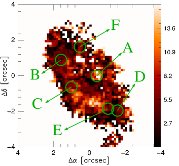
Figure 6.— $A_{V}$ gas extinction map of NGC 5135 based on Br$\gamma$/Br$\delta$ line ratio. The arrows show our six selected regions A-F and the circles approximately represent the apertures in K-band. White regions are those with unreliable $A_{V}$ measurements in individual spaxels. The Calzetti et al. (2000) extinction law has been assumed.

As we can see from Fig. 6, the regions with higher $A_{V}$ values are:

(i) The Nuclear Region: The average visual extinction is about 10 mag (0.9 mag at 2.2 $\mu$m), with a local peak reaching the maximum of our scale at about 17 mag. This result is consistent with the conclusions of González Delgado et al. (1998). At least qualitatively, it is also in agreement with findings of Levenson et al. (2004) using Chandra X-ray data. They claim that the nuclear AGN engine must be obscured by a high hydrogen column density ($N_{H}\rm\geq 10^{24}\,cm^{-2}$, having in mind they have used $4\times$ larger apertures than ours). Although we do not find such high $N_{H}$ values (see Sec. 3.5.2, Table 4), our $1$-$\rm 3\times 10^{22}\,cm^{-2}$ measurements in region A are by far the highest of our A-F apertures.

(ii) A region south from the nucleus ($\Delta\alpha\approx[-0.5,1.0]$, $\Delta\delta\approx[-2.0,-1.0]$, approx.): It has a mean visual extinction of 10 mag. Presenting some local peaks of about 17 mag, this area covers the space between our regions C and E. No strong emission in Br$\gamma$, Br$\delta$ and HeI flux maps is observed in this area, but only a weaker, smooth component at SINFONI’s resolution. Despite the fact that both Brackett lines are clearly detected in this zone, we cannot discard that some of the peaks might be partially produced by flux uncertainties, particularly of the Br$\delta$ line and its complex local continuum determination. A higher continuum level estimation would decrease this line flux, therefore, artificially increasing the extinction (see eq. 1). In any case, because this region does not match with our A-F zones, it will not affect our extinction corrected fluxes (Table 7) and conclusions derived from them.

The rest of the map presents a median visual extinction of 6 mag which translates into 0.55 mag at 2.2 $\mu$m.

Alonso-Herrero et al. (2006a) presented an F110W-F160W color map of NGC 5135 (using NICMOS-NIC2; similar to J-H color) which can be interpreted as a stellar extinction map to a first order. It is difficult, however, to directly translate this map to $A_{V}$ extinction to the stars, mainly because we have to assume an age for the stellar population (to get its theoretical J-H color) in a galaxy which may have a composite stellar population (see Secs. 3.3.1 and 3.4). In terms of their structure, a comparison between Fig. 6 and Alonso-Herrero et al. color map shows that they are remarkably different. While both maps seem to agree in having the larger extinctions around the nucleus, the color map clearly traces the nuclear spiral arms while no sign of this is observed in our $A_{V}$ map. We do not think that the higher spatial resolution of NICMOS data can totally explain such a radical mismatch by itself. Instead, the close wavelength proximity between our two Brackett emission lines might be the responsible of the apparent $A_{V}$ map lack of structure. The similar extinctions for both Brackett emission lines produce $A_{V}$ values (from eq. 1) very sensitive to small flux uncertainties. Therefore, the detailed structure in the $A_{V}$-gas map gets easily lost within Br$\gamma$ and Br$\delta$ errors. We remark, however, that for larger areas (sampled by few tenths of spaxels like regions A-F), the mean $A_{V}$ values should be a reasonably good estimation of the local internal extinction.

3.3. Ionization Mechanisms of Gas

The presence of ionized gas is usually interpreted as a tracer of recent star formation, where UV radiation from massive O-B stars is capable of keeping the surrounding gas in an ionized state. In the NIR, recombination lines like Pa$\alpha$ and Br$\gamma$ are frequently used as tracers of this activity.

However, there are other mechanisms capable of ionizing the ISM. Shocks produced in SNR can partially ionize the gas. In the NIR, SNRs can be traced by the [FeII]${\rm\lambda 1.26\,\mu m}$ and [FeII]${\rm\lambda 1.64\,\mu m}$ lines (e.g. Greenhouse et al. 1991, Alonso-Herrero et al. 2003). A strong [FeII] flux is not expected in normal H ii regions (Mouri, Kawara & Taniguchi 2000): their abundant fully-ionized hydrogen would produce Fe atoms in higher ionization states. Therefore, by using our Br$\gamma$ and [FeII]${\rm\lambda 1.64\,\mu m}$ fluxes we are tracing different ionization mechanisms with also different ionization efficiencies.

In Fig. 7 we present the extinction corrected [FeII]/Br$\gamma$ flux map. This diagnostic allows to see which ionization mechanism is more dominant in different regions of the galaxy. An [FeII]/Br$\gamma$ ratio $\lesssim 1$ is usually taken as characteristic of a starburst, while much larger values are associated with only partially ionized regions by shocks (e.g. Graham et al. 1987, Kawara et al. 1988, Mouri et al. 1990, Alonso-Herrero et al. 1997, 2001).

3.3.1 Circumnuclear Starforming Regions

Fig. 7 shows that only three regions (associated to B, C and D) seem to have a non-negligible contribution from starburst activity. In the same figure, we overplot in contours the EW(Br$\gamma$) as an upper-limit age indicator. It is clear that the EW(Br$\gamma$) peaks match very well those areas with low-[FeII]/Br$\gamma$ ratio, pointing out that a young stellar population contributes to ionize the ISM in these areas. We have tested this idea by using the SB99 models with instantaneous star formation, solar metallicity and Kroupa initial mass function (hereafter IMF). In Table 1 we present the predicted ages (upper limits) of the stellar populations for our selected regions, derived from our EW(Br$\gamma$) measurements of Table 7. As we can see, B, C and D are the three youngest areas with $\rm\approx 6\,Myr$ old, while E and F are slightly older. These results are consistent with previous findings with UV/visual data (González Delgado et al. 1998). It is possible that some contamination from the nearby starburst regions has been introduced within E and F zones, particularly for the former.

Table 1StarBurst 99 Ages from EW(Br$\gamma$)

Reg	Agea [Myr]
A	$\leq 7.02$
B	$6.15_{-0.03}^{+0.02}$
C	$6.38_{-0.43}^{+0.03}$
D	$6.14_{-0.03}^{+0.02}$
E	$6.52_{-0.03}^{+0.04}$
F	$6.51_{-0.05}^{+0.04}$

(^a) Ages with their $\pm 1\sigma$ errors. Ages should be considered as upper limits only. See text for details and footnote 3 for region A.

A plausible explanation for the local [FeII]/Br$\gamma$ variations might be suggested from Table 1 ages, where regions E and F are marginally older than the others. According to models, after about $\rm 6$-$\rm 7\,Myr$ important changes start taking place in young stellar populations. The massive O-B stars responsible for most of the Br$\gamma$-emission explode as SNe, diminishing this flux feature in the integrated spectra. On the other hand, after $\rm\sim 4\,Myr$ since the starburst, the SNe rate has been increasing dramatically, enriching the ISM with Fe. Therefore, two different processes radically change the [Fe/H] abundance and the Br$\gamma$ flux: when total ionization from O-B stars leaves place to partial ionization from SNR shocks, the Fe-enriched ISM increases the [FeII] flux, while the decline of O-B stars decreases Br$\gamma$. If a certain region has not reached yet this crucial stage on its stellar evolution (like B, C and D) we would observe low [FeII]/Br$\gamma$ ratios. On the other hand, if the stellar population has reached this point (like in E and F), much higher [FeII]/Br$\gamma$ ratios would be observed.

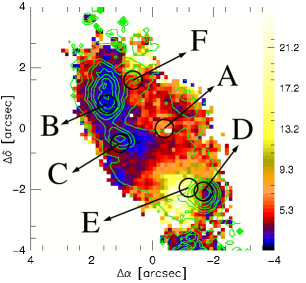
Figure 7.— Extinction corrected [FeII]/Br$\gamma$ line ratio map. In contours we plot the EW(Br$\gamma$) as an age indicator. The arrows show our six selected regions A-F and the circles approximately represent the apertures in K-band.

The high values of [FeII]/Br$\gamma$ ($>$ 20) in regions E and F are, in fact, very similar to those observed in SNRs, e.g. $\sim 30$ in IC 443 (Graham et al. 1987) or 34 in RCW 103 (Oliva et al. 1989). In the FWHM([FeII]) map of Fig. 3 we see that both sources are the only ones with very high values (or large velocity dispersions). This would be, in principle, in excellent agreement with a scenario where SNR shocks have perturbed the kinematics of these areas.

We have compared all our [FeII]/Br$\gamma$ measurements with predictions from the SB99 models. On its latest versions, SB99 does not give directly the [FeII] fluxes but the SNe rate. So we transform these values to [FeII] flux by using empirical relations from Calzetti (1997) and Alonso-Herrero et al. (2003). By using these expressions, we can further test (to first order) the SNR scenario. See Sec. 3.6 for further discussion about SNe rate estimations. In Fig. 8 we present SB99 predictions with the two empirical relations mentioned above. We overplot our measured [FeII]/Br$\gamma$ ratios for A-F with their uncertainties. We have used the upper-limit ages of Table 1 to fix the abscissa of our data points.

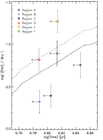
Figure 8.— [FeII]/Br$\gamma$ vs. Age (upper limits from EW(Br$\gamma$)) for our six regions. Based on SB99 models, different relations have been used to derive the [FeII] flux from the SNe rate: dashed line, Calzetti (1997); solid line, Alonso-Herrero et al. (2003).

Only regions D and F show a clear agreement with the SNR models at those ages. Region D has an important [FeII] emission contribution from the broad peak traced by region E. So, the agreement between this young starburst region and the models is not surprising. The good match with F only reinforces the link between this area and SNRs as mentioned before using kinematic arguments. The starburst B and C regions lay below model predictions, pointing towards pure stellar photodissociation mechanisms as the responsible of the gas ionization.

Certainly, the most interesting outlier is region E, where the models predict a smaller [FeII]/Br$\gamma$ ratio than observed. This implies that an additional ionization source must be invoked to explain the observations at the center of this resolved [FeII] peak (region D, taken as a peripheral sample of this peak, does not need such an extra ionization source). A plausible alternative comes from X-ray photoionization. As mentioned in previous sections, Levenson et al. (2004) have published Chandra X-ray data for NGC 5135. They have identified in their total band map ($0.4$-$\rm 8\,keV$) a strong emission corresponding to region E. According to these authors, the non-thermal component (power law and the bulk of the hard X-ray emission) is likely to be associated to X-ray binaries in the starburst, while the thermal one (most of the soft emission) is typical of a starburst galaxy. These mechanisms may explain the difference between models and E data in Fig. 8, where both, X-rays and SNR shocks are contributing to the observed [FeII]/Br$\gamma$ ratio.

3.3.2 The Ionization Cones and Central AGN

The central region A of NGC 5135 deserves a separate section given its particular characteristics with respect to the other starforming regions.

As mentioned in previous sections, the AGN activity has been traced by the [SiVI] coronal line. The [SiVI]-luminosity for this region is $\rm L_{[SiVI]}=3.6\times 10^{39}\,erg\,s^{-1}$, in agreement with similar measurements in other local Seyfert 2 galaxies, like Circinus, NGC 1068, NGC 3227 and Mrk 609 which span a range $\sim 10^{39}$-$\rm 10^{40}\,erg\,s^{-1}$ (the two later objects are Seyfert 1.5 and 1.5-1.8, respectively; Rodríguez-Ardila et al. 2006a, Zuther et al. 2007).

By using Br$\gamma$-emission, we can make a row estimation of the AGN contribution to the gas photoionization. If we assumed that the (extinction corrected) Br$\gamma$ flux in region A is entirely produced by the AGN, we can compare this value with the total Br$\gamma$ flux in our FoV. According to this, the AGN contributes in $\rm\lesssim 3\%$ of the gas photoionization within the central $\rm 2.3\,kpc$ of this galaxy. By doing a similar calculation, we also estimate that the AGN represents $\rm\lesssim 3$ and $\rm\lesssim 5\%$ of the NIR-luminosity in the ${\it H}$- and ${\it K}$-bands, respectively.

Concerning the ionization mechanisms, on the one hand the AGN embedded in this zone is likely to play an important role at local level by photoionizing the gas in the nuclear neighborhood (Marconi et al. 1994, Ferguson et al. 1997, Contini et al. 1998, see also Rodríguez-Ardila et al. 2006b and references therein). The [FeII]/Br$\gamma$ = 5.7 measured in this region is consistent with typical Seyfert galaxy values from a compilation of different object types shown in Alonso-Herrero et al. (1997).

The “plume” shape structure in [SiVI]-emission (NE of the nucleus, Sec. 3.1.1, Fig. 3) probably traces the direction of a cone, pointing that the AGN is also capable to ionize the ISM at larger distances. The presence of shocks from outflowing winds would produce such ionized plasma and cone-features (Viegas-Aldrovandi & Contini 1989). The [SiVI]-emission is particularly broad in A with a FWHM of $\rm\approx 28\,\AA$ (or $\rm\approx 430\,km\,s^{-1}$), strengthening the idea of an important interaction between AGN outflows and the surrounding material. It is interesting to notice that the FWHM([SiVI]) nuclear peak structure extends approximately along the semi-minor axis as expected in outflow models of Heckman et al. (1990). This may suggest the presence of multiple components in the [SiVI] kinematics. The high FWHM(Br$\gamma$) in this area ($\rm\approx 22\,\AA$ or $\rm\approx 300\,km\,s^{-1}$) is also consistent with this hypothesis. In Paper II we will find out if this scenario receives further support from our detailed kinematical study. The NE [SiVI] structure has a SW counterpart not detected on a spaxel-by-spaxel basis. By integrating few spaxels at $2^{\prime\prime}$ SW from the nucleus, we have detected clear [SiVI]-emission which is absent in other areas close to region A. This SW component is probably weaker because of extinction and projection effects.

On the other hand, in Levenson et al. (2004) work on X-rays, the authors have found the strongest emission peak in our region A, which may also contribute to the ionization in this area. They suggest, however, that the bulk of the thermal (collisional) X-ray emission, even in the nucleus, is stellar, not due to the AGN. In principle, this would be understood in terms of the larger apertures they use in A (about $4\,\times$ ours) within which a stronger stellar component, that we miss, might be introduced. However it is also true that compact starforming regions have been usually found in AGN’s neighborhood at distances of tens of pc (e.g. González Delgado et al. 1998, Weaver 2001, Davies et al. 2007). Considering the significant dilution from the AGN, the later point is reinforced for NGC 5135 by our findings of NaI and CO stellar absorption in this zone.

Therefore in region A and in the [SiVI]-cone the AGN photoionization and outflows seem to play an important role on ionizing the gas. However, a stellar contribution cannot be totally discarded, particularly in region A. Then, it is comprehensible why in Fig. 8, the starburst-based models cannot reproduce the observed [FeII]/Br$\gamma$ ratio of this region, in addition to the age uncertainty in this zone.

Finally, the remaining extended emission in Fig. 7 has rather large [FeII]/Br$\gamma$ ratios, typically between 3 and 7. This suggests that the ISM gas is mainly ionized by other mechanisms (e.g. SNR shocks, X-rays) instead of photodissociation from star formation.

3.4. Dating the Stellar Population: Further constrains from Absorption Lines

In the previous section, we have studied a young stellar population ($\rm\leq 7\,Myr$) with either an important fraction of O-B stars or in a transition period with high SNe rates. We attempted to understand its importance on ionizing the ISM gas by both, the use of the [FeII]/Br$\gamma$ map structure, and the estimation of the stellar population age. Because of this, we now consider appropriate to introduce at this point the analysis of the stellar population traced by the NIR-continuum and CO$\lambda 2.29\mu$m absorption maps of Fig. 4. By doing this, we will address the open issues presented in Sec. 3.1.5.

In Fig. 4, we have seen that NIR-continuum and CO$\rm\lambda 2.29\,\mu m$ maps have a very similar structure everywhere but in region A. The absence of a strong central peak in the CO flux map can be explained by the influence of the AGN in the stellar continuum. The strong X-ray/UV radiation from AGN is reprocessed by the surrounding dust grains and re-emitted in the IR (e.g. Clavel et al. 1992, Forbes et al. 1992). Therefore, the continuum flux in H and K-bands increases, diluting the CO and other stellar absorption features. The high extinction we estimate for this area (see also Alonso-Herrero et al. 2003) and the finding of hot dust emission ($\sim 200\,$K) in the nucleus of NGC 5135 (Gemini/T-ReCS N-band data, Alonso-Hererro et al. 2006b) are consistent with this idea. The high temperatures required for the dust to emit in K-band, however (1200-1500 K; e.g. Clavel et al. 1989, Glass 1992, Rodríguez-Ardila et al. 2005a, 2006b), limit this effect to rather short distances from the AGN ($\leq 100\,$pc; Marco & Alloin 1998, 2000). In fact, the observed dilution towards the center of the EW(CO) map (Fig. 4, bottom-right panel) occurs at similar distances of about $0.4^{\prime\prime}$ ($\sim\rm 120\,pc$). This apparently close agreement, however, is almost certainly driven by PSF effects. It is possible than hot dust emission is confined to even shorter distances from the active nucleus. In regions farther away from the nucleus ($\gtrsim 200\,$pc) the EW(CO) values are free of the AGN contamination and can be confidently used for further tests of the stellar population properties.

As for A-F zones, we extracted integrated spectra for other three extra-nuclear regions labeled as X, Y and Z (see Fig. 4, top-left panel). They do not match with our A-F apertures but coincide with the three extra-nuclear peaks of the NIR-continuum (this is clearly shown in Fig.5) where the CO signal is higher. Our aim is to do a general comparison between the young and (potentially) old stellar populations for the entire galaxy, based on individual regions where one or the other is dominant. In this way, we base our conclusions on higher S/N data.

We estimate the stellar population ages in X-Z by using the EW(CO$\lambda 2.29\,\mu$m) and the models SB99 and STARS (Sternberg 1998, Thornley et al. 2000, Davies et al. 2003). Both models include treatments for the thermally pulsing AGB stars. However, without knowing parameters like the metallicity and characteristics of the star formation history, the model predictions might vary from case to case. We have run these models using different IMFs (Kroupa, Salpeter) and metallicities (0.04, 0.02, 0.008) without finding substantial variations which may change our conclusions. Therefore we have assumed solar metallicity, Kroupa IMF and the Genova isochrons for all our age predictions. Only the use of different star formation histories (instantaneous and continuous) has a relevant impact on this respect. We will discuss this particular point in the following paragraphs.

Strictly speaking, STARS makes use of exponentially decaying star formation rates (hereafter SFRs). However, by using a long characteristic time-scale ($\rm 1000\,Gyr$) we recover a continuous SFR, while by using a short one we basically recover instantaneous burst results for ages $\rm\geq 1\,Myr$. We can directly compare this models to instantaneous and continuous SFR models from SB99 (R. L. Davies, private communication).

In Table 2 we present instantaneous-burst model results for regions X-Z. Because SB99 and STARS models interpolate the EWs from spectral grids, their predictions become quite noisy at larger ages ($\geq\rm 100\,Myr$), particularly for STARS were a template star library is used (see Fig.9; R. L. Davies, private communication). Therefore, in cases of old stellar populations ($\geq\rm 100\,Myr$) a range of ages is presented for SB99, while lower limits are shown when STARS is used.

Table 2CO$\lambda 2.3\,\mu$m, NaI$\lambda 2.21\mu$m and $\rm Br\gamma$ EWs and Instantaneous burst model ages for regions X-Z

Reg	EW(CO)	$\rm Age1_{SB99}^{CO}$	$\rm Age1_{\tt STARS}^{CO}$	$\rm Age2_{SB99}^{CO}$	$\rm Age2_{\tt STARS}^{CO}$	EW(NaI)	$\rm Age1_{\tt STARS}^{NaI}$	$\rm Age2_{\tt STARS}^{NaI}$	EW($\rm Br\gamma$)	$\rm Age_{SB99}^{\rm Br\gamma}$
	[Å]	[Myr]	[Myr]	[Myr]	[Myr]	[Å]	[Myr]	[Myr]	[Å]	[Myr]
X	6.44 $\pm$ 0.4	$7.37_{-0.03}^{+0.03}$	$7.01_{-0.08}^{+0.05}$	213-453	$\geq$ 200	1.76 $\pm$ 0.08	$8.20_{-0.06}^{+0.06}$	$\geq$ 200	6.01 $\pm$ 0.64	$6.80_{-0.05}^{+0.06}$
Y	7.14 $\pm$ 0.3	$7.42_{-0.02}^{+0.02}$	$7.14_{-0.05}^{+0.05}$	205-211	$\geq$ 200	1.99 $\pm$ 0.07	$8.38_{-0.06}^{+0.04}$	$\geq$ 200	7.15 $\pm$ 0.53	$6.70_{-0.03}^{+0.05}$
Z	6.90 $\pm$ 0.3	$7.40_{-0.02}^{+0.03}$	$7.10_{-0.10}^{+0.05}$	205-445	$\geq$ 200	1.88 $\pm$ 0.08	$8.29_{-0.06}^{+0.06}$	$\geq$ 200	6.64 $\pm$ 0.57	$6.74_{-0.04}^{+0.05}$

As we can see in Fig.9 (upper panel), instantaneous-burst models produce two possible stellar population ages consistent with our data (around $\rm 7$ and $\rm\geq 200\,Myr$, respectively), while continuous-star-forming ones produce a single range of ages around $\rm 7\,Myr$. Although a stellar population of $\rm\sim 7\,Myr$ would agree with our findings in B-F zones using $\rm EW(Br\gamma)$, the presence of a second, totally different population receives support from two different sources.

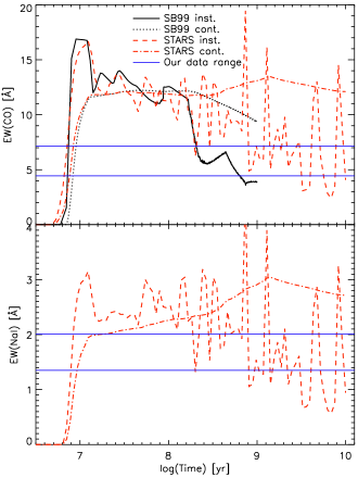
Figure 9.— SB99 and STARS model predictions for EW(CO) and EW(NaI). The two horizontal lines represent the range of our data for regions A-F and X-Z.

First of all, our CO-flux (Fig. 4 bottom left panel) and $\rm Br\gamma$-emission maps (Fig. 3 top of first column) clearly trace different structures (peaks) in this galaxy, usually separated by more than $\rm 200\,pc$ in projection. On the other hand, the CO-flux map almost mimics the structure observed in the NIR-continuum, which in turn is frequently used as a tracer of more evolved stellar populations than those with high $\rm EW(Br\gamma)$. Further support for this argument comes from Alonso-Herrero et al. (2006a) NICMOS/$HST$ data of this galaxy (see Alonso-Herrero et al. 2006b, Fig. 1 second row for sharper figures). The higher spatial resolution of their NIR-continuum and Pa$\alpha$-emission maps show the peaks observed with SINFONI actually have a complex structure. Moreover, the NICMOS continuum and Pa$\alpha$ peaks are not coincident spatially, demonstrating that, between the neighbouring aperture pairs X-B, Y-C and Z-D, we are picking-up different spatially resolved regions (even though some PSF-contamination effects between aperture pairs). In terms of structure, further support to spatial variations in the stellar population comes from the EW(CO) map (Fig. 4 bottom right panel). This figure shows a clear radial (projected) distinction in function of EW. While at distances of $\rm\sim 600\,pc$ from the nucleus we find $\rm EW(CO)\sim 7\,\AA$, this value decreases to $\rm\sim 5\,\AA$ at $\rm\sim 300\,pc$. Such spatial segregation supports the idea of a change in the stellar population properties (e.g. a variation in the relative contribution of red giants and supergiants to the integrated light).

Secondly, the EW of different spectral features also point towards different stellar populations in X-Z with respect to B-D zones. On the one hand, the EW(CO) of the former are larger than those for the later as we can see in Tables 2 and 7, respectively. The quoted uncertainties show that these differences are significant at a $4$-$5\,\sigma$ level. We observe the EW differences are mainly driven by CO-absorption variations rather than continuum-level changes. This suggests the existence of a different stellar population in X-Z with respect to B-D, the former regions having a more important red giant/supergiant contribution to the integrated spectra (e. g. Origlia & Oliva 2000). On the other hand, as we can see in Tables 2 and 7, the EW(Br$\gamma$) is substantially lower in regions X-Z than in B-D zones, also pointing towards two different populations. Putting together all the observational evidence, the NIR-continuum and CO-absorption (red giant/supergiant stars) and $\rm Br\gamma$-emission (O-B stars) suggest the existence of (at least) two stellar populations in this galaxy.

However, as mentioned above, the stellar population model predictions are not that clear about this point, depending on the star formation history used (see Fig.9). If we assume continuous SFR models, the EW(CO) for all our apertures are consistent with a $\rm\sim 7\,Myr$ old population. By using the $\rm EW(Br\gamma)$ with the same models, however, we get different results. The B-D regions are now consistent with a $\rm 10\,Myr$ old stellar population, while regions X-Z are better constrained by a $\rm\sim 60\,Myr$ old one. Clearly, the use of continuous models with the measured EWs produce inconsistent results between the two tracers.

Instead, if we use instantaneous SFR models, the observed EW(CO) are consistent with two populations of $7$-$8$ and $\rm\geq 200\,Myr$ old, respectively (see Table 2 and 3 for regions X-Z and B-F, respectively). This degeneracy is broken by using $\rm EW(Br\gamma)$. Even though regions X-Z have much smaller $\rm EW(Br\gamma)$ values than B-D, all these zones are consistent with a 6-$\rm 7\,Myr$ stellar population according to models (Tables 2 and 3). In this case, the instantaneous model predictions are consistent between our different EW measurements.

Table 3CO$\lambda 2.3\,\mu$m and NaI$\lambda 2.21\mu$m Instantaneous burst model ages for regions B-F

Reg	$\rm Age1_{SB99}^{CO}$	$\rm Age1_{\tt STARS}^{CO}$	$\rm Age2_{SB99}^{CO}$	$\rm Age2_{\tt STARS}^{CO}$	$\rm Age1_{\tt STARS}^{NaI}$	$\rm Age2_{\tt STARS}^{NaI}$
	[Myr]	[Myr]	[Myr]	[Myr]	[Myr]	[Myr]
Ba	$7.26_{-0.02}^{+0.02}$	$6.72_{-0.06}^{+0.06}$	534-592	$\geq$ 811	$7.89_{-0.05}^{+0.05}$	$\geq$ 200
C	$7.33_{-0.02}^{+0.03}$	$6.91_{-0.06}^{+0.06}$	217-509	$\geq$ 200	$8.05_{-0.05}^{+0.05}$	$\geq$ 200
Da	$7.30_{-0.03}^{+0.03}$	$6.82_{-0.07}^{+0.08}$	233-552	$\geq$ 811	$8.11_{-0.08}^{+0.07}$	$\geq$ 200
E	$7.41_{-0.03}^{+0.03}$	$7.12_{-0.07}^{+0.07}$	200-443	$\geq$ 200	$8.39_{-0.07}^{+0.07}$	$\geq$ 200
Fa	$7.22_{-0.02}^{+0.03}$	$6.61_{-0.07}^{+0.08}$	581-698	$\geq$ 811	$8.01_{-0.08}^{+0.08}$	$\geq$ 200

We have also compared the EW(NaI$\lambda 2.21\mu$m) measurements with STARS model predictions. All previous warnings and discussion about the EW(CO) age estimation are also applicable to this stellar absorption feature. As we can see in Fig.9 bottom panel and in Tables 2 and 3, the younger-age predictions for an instantaneous model are somehow larger ($\rm\sim 8\,Myr$) than those with EW(CO), but still consistent with a young population.

In summary, while observational evidence points towards two different stellar populations, the model predictions cannot clearly discriminate between them. Our measurements are consistent with temporally close, instantaneous bursts occurred $6$-$\rm 8\,Myr$ ago. Strictly speaking, regions X-Z are always older than their neighbors B-D (independently of the tracer used) by few hundred thousand years. Even though it is worth mentioning, such small age differences might be in the limit of current model capabilities for discriminating between two stellar populations. Certainly, we cannot discard the possibility of two populations of similar ages: a young one ($\rm\sim 7\,Myr$) dominated by O-B stars and an intermediate-age one ($\rm\sim 10\,Myr$) with massive stars which already started their evolution to red supergiants. In such particular case, the presence of local metallicity variations between regions might become an issue given the tight correlation between the CO-index and metallicity (Origlia & Oliva 2000). In any case, given the above discrepancies, we cannot be conclusive about the existence of one or more stellar populations and thus, further data and tests are necessary to shed light about this issue.

3.5. H₂ Excitation Mechanisms

Different mechanisms have been proposed to be responsible of the H₂ excitation and literature is rich in examples where more than one process is shaping the observed emission spectra (e.g. Draine & Woods 1990; Mouri 1994; Davies, Sugai & Ward 1997; Quillen et al. 1999; Burston, Ward & Davies 2001; Davies et al. 2005; Rodríguez-Ardila et al. 2005b; Zuther et al. 2007). Between these mechanisms, the most commonly discussed are UV-fluorescence (photons, non-thermal), shock fronts (collisions, thermal) and X-ray excitation (collisions through secondary electrons, thermal).

In this section, we will focus on trying to understand the observed H₂-emission by using different diagnostic diagrams. We will consider both non-thermal and thermal excitation mechanisms and models in the analysis.

3.5.1 H₂ Line Ratios: A Diagnostic Diagram

As a first step, we have calculated different H₂-emission line ratios for our six regions in NGC 5135. As mentioned in Sec. 2.5, we did not use fluxes corrected for extinction. Different models and data suggest that the excitation mechanisms mentioned above produce characteristic line ratios between different roto-vibrational transitions (see Fig. 10). In this sense, the many lines presented in our ${\it K}$-band data allowed us to use a line-ratio diagnostic diagram for our analysis. We maximise the difference between thermal and non-thermal processes by trying to remove the ortho/para ratio effect (ratio equal to 3 for a thermal distribution and $<3$ for a non-thermal one). We adopt the intensity ratios 2-1 S(1)/1-0 S(1) and 1-0 S(3)/1-0 S(1) to achieve this goal. Given that the 2-1 S(1), 1-0 S(3) and 1-0 S(1) lines occur in ortho-molecules only, the non-thermal values of their ratios are supposed to be constant (Mouri 1994).

In Fig. 10 we present the line-ratio diagnostic diagram for our six regions compared with different models and data from literature. The first obvious conclusion from this diagram is that none of our six regions seem to be dominated by non-thermal (fluorescence) excitation. Instead, they lie closer to thermal processes like X-ray heating and SNR shocks, the most likely dominant mechanisms responsible of H₂ excitation in the six zones. Regions B and D, however, clearly depart from the pure thermal emission curve suggesting some UV-fluorescence contribution to the observed lines. This is reasonable in principle given that B and D correspond to recent star forming regions where UV-photons are abundant. The remaining four regions (A, C, E and F) are consistent with the purely thermal emission curve (within the uncertainties) with gas temperatures between 2000 and 3000 K. The overall lack of dependence on UV-processes (i. e. recent star formation) agrees with the comparison between our Br$\gamma$ and H2 flux maps (Fig. 3). The clear structural differences between them implies that the processes exciting the H2 gas are not those who produce Br$\gamma$ (i. e. recent star formation).

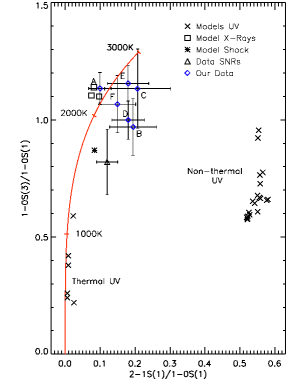
Figure 10.— H₂ diagnostic diagram using the 2-1 S(1)/1-0 S(1) and 1-0 S(3)/1-0 S(1) intensity line ratios. Diamonds represent our own data for the six selected regions of NGC 5135. The $\times$ symbols represent thermally (Sternberg & Dalgarno 1989) and non-thermally (Black & van Dishoeck 1987) UV-exited models. Squares correspond to X-ray heating models of Draine & Woods (1990). The asterisk is a shock model from Brand et al. (1989). The triangle is SNR data from Oliva, Moorwood & Danziger (1990). The curve represents thermal emission between 0 and 3000 K (eqs. 2 and 3, see references in the text).

By comparing with models, it is interesting to notice that region A, the AGN nucleus, matches very well with the X-ray models of Draine & Woods (1990). As mentioned in previous sections, Levenson et al. (2004) have found a strong X-ray source in this area. In their discussion, Draine & Woods (1990, 1991) argued that there is a range of values of X-ray energy per volume for which the gas gets sufficiently hot to vibrationally excite the H₂ (producing the observed H₂ lines with high enough efficiency to be observed), but not hot enough to dissociate it. They proposed the X-ray emission from SNRs (and not their shocks) as one plausible stellar energy source. This scenario implies other constraints like high gas densities ($n_{H}\geq 10^{5}\,\rm cm^{-3}$, attainable in the dense circumnuclear regions around AGNs) and high SNe rates (e.g.  $\rm\approx 1.5\,yr^{-1}$ within the central $\rm 4\,kpc$ of NGC 6240, but with high uncertainties). The later constraint seems to be achieved by NGC 5135, with a SNe rate of $\rm\sim 0.4$-$\rm 0.6\,yr^{-1}$ within the central $\rm 2.3\,kpc$ (see Sec. 3.6 for further details). As an extra possible piece of evidence, the Draine & Woods’ models predict a decrement in the 2-1 S(3) transition flux ($v=2$, $J=5$ level), which we actually observed in Fig. 11 (within large uncertainties).

We also highlight in Fig. 10 that region E is consistent with a thermal process but far from the SNR data and shock model. As we saw in Sec. 3.3, SNR shocks were an important candidates for H₂-excitation given the high [FeII] fluxes and FWHMs observed in this area. Could region E be in a similar scenario to the one described above for A? Certainly, the X-ray models are not as close to E as to region A, however we know from Levenson et al. (2004) work that the second X-ray peak comes from region E and it has a star formation origin. In principle, the same arguments presented before for region A might be applied to E in the sense that an important fraction of H₂ excitation might be produced by X-rays of stellar origin.

Finally, region F is also consistent with thermal processes. However, the uncertainties make it difficult to distinguish between X-ray and SNR shock scenarios. Because the later has a dominant role in ionizing the local ISM gas (Sec. 3.3.1), SNR shocks become a likely candidate to dominate the H₂ local excitation in this area.

3.5.2 H₂ population diagram

Because we are able to measure H₂-emission lines from different vibrational transitions (1-0 and 2-1), we adopt another approach to characterise the observed excitation mechanisms. We have just seen in Sec. 3.5.1 that the dominant processes responsible for H₂ excitation are thermal (collisional). Therefore, if we assume pure thermal excitation, the different roto-vibrational levels are populated as described in the Boltzmann equation. This allowed us to represent the different transitions as a function of their population (probability) densities versus the energy of the upper level, in what is called a population diagram. For a thermally excited gas, all the transition values lie on a straight line and the corresponding slope is inversely proportional to the H₂ gas temperature.

Given that molecular gas clouds contain a large number of molecules, the population densities are essentially proportional to the observed column densities. So, the probability ratio between two different states can be expressed with the Boltzmann equation as

$$\frac{P_{a}}{P_{b}}=\frac{N(v,J)_{a}}{N(v,J)_{b}}=\frac{g_{a}\cdot e^{-E_{a}/kT}}{g_{b}\cdot e^{-E_{b}/kT}}$$ (2)

where $P_{a}$ and $P_{b}$ are the probabilities of finding an H-molecule in any of the degenerate states ($g_{a}$, $g_{b}$) with energy $E_{a}$, $E_{b}$. $N(v,J)_{a}$ and $N(v,J)_{b}$ are the observed column densities at the corresponding states, $v$ and $J$ are the vibrational and rotational quantum numbers, respectively. $k$ is the Boltzmann constant and $T$ is the gas temperature. The column densities can be derived with the formula:

$$N(v,J)=\frac{f}{A(v\,J,v^{\prime}\,J^{\prime})}\times\frac{\lambda}{hc}\times\frac{4\pi}{\Omega_{aper}}$$ (3)

where $f$ is the measured flux for the corresponding emission line, $A(v\,J,v^{\prime}\,J^{\prime})$ is the transition probability from the $(v\,J)$ to the $(v^{\prime}\,J^{\prime})$ quantum state (taken from Wolniewicz et al. 1998), $\lambda$ is the rest frame line wavelength, $h$ is the Planck constant, $c$ is the speed of light and $\Omega_{aper}$ is the squared aperture diameter of $\rm 0.^{\prime\prime}62$. The derived column densities for each H₂ indicator and region are presented in Table 4.

Table 4H₂ column densities derived for six regions in NGC 5135.

	Region A		Region B		Region C		Region D		Region E		Region F
Line	$N_{H,obs}^{a}$	$N_{H,cor}^{b}$	$N_{H,obs}^{a}$	$N_{H,cor}^{b}$	$N_{H,obs}^{a}$	$N_{H,cor}^{b}$	$N_{H,obs}^{a}$	$N_{H,cor}^{b}$	$N_{H,obs}^{a}$	$N_{H,cor}^{b}$	$N_{H,obs}^{a}$	$N_{H,cor}^{b}$
	[$\rm 10^{21}cm^{-2}$]		[$\rm 10^{21}cm^{-2}$]		[$\rm 10^{21}cm^{-2}$]		[$\rm 10^{21}cm^{-2}$]		[$\rm 10^{21}cm^{-2}$]		[$\rm 10^{21}cm^{-2}$]
1-0 S(0)	3.49	9.35	1.11	1.87	0.88	1.60	1.57	2.36	1.93	3.13	0.85	1.51
	$\pm$0.66	$\pm$ 2.17	$\pm$0.26	$\pm$0.49	$\pm$0.28	$\pm$0.56	$\pm$0.30	$\pm$0.54	$\pm$0.38	$\pm$0.73	$\pm$0.20	$\pm$0.41
1-0 S(1)	10.54	30.38	2.78	4.85	2.45	4.68	4.51	6.97	6.94	11.65	2.37	4.38
	$\pm$0.46	$\pm$4.64	$\pm$0.22	$\pm$0.78	$\pm$0.25	$\pm$0.81	$\pm$0.24	$\pm$1.05	$\pm$0.33	$\pm$1.73	$\pm$0.18	$\pm$0.73
1-0 S(2)	3.16	9.78	0.90	1.63	1.07	2.13	1.33	2.12	2.41	4.20	0.83	1.60
	$\pm$0.40	$\pm$ 1.96	$\pm$0.21	$\pm$0.45	$\pm$0.27	$\pm$0.63	$\pm$0.21	$\pm$0.46	$\pm$0.30	$\pm$0.82	$\pm$0.17	$\pm$0.41
1-0 S(3)	9.10	30.20	2.05	3.86	2.11	4.40	3.43	5.62	6.11	10.99	1.93	3.86
	$\pm$0.38	$\pm$5.17	$\pm$0.19	$\pm$0.71	$\pm$0.23	$\pm$0.85	$\pm$0.21	$\pm$0.96	$\pm$0.29	$\pm$1.82	$\pm$0.16	$\pm$0.72
2-1 S(1)	0.77	2.04	0.40	0.66	0.38	0.68	0.60	0.90	0.92	1.48	0.26	0.46
	$\pm$0.25	$\pm$ 0.70	$\pm$0.13	$\pm$0.24	$\pm$0.17	$\pm$0.31	$\pm$0.15	$\pm$0.25	$\pm$0.30	$\pm$0.52	$\pm$0.09	$\pm$0.17
2-1 S(3)	0.54	1.64	0.25	0.44	0.15	0.29	0.26	0.42	0.38	0.64	0.16	0.29
	$\pm$0.22	$\pm$ 0.70	$\pm$0.11	$\pm$0.21	$\pm$0.12	$\pm$0.24	$\pm$0.10	$\pm$0.17	$\pm$0.15	$\pm$0.27	$\pm$0.08	$\pm$0.16

(^a) Total column densities derived by using the observed H₂ line fluxes. Below the main values, their $\pm 1\,\sigma$ errors.
(^b) Total column densities after extinction correction for each observed H₂ line and region as listed in Table 7. Below the main values, their $\pm 1\,\sigma$ errors.

By taking the logarithm in eq. 2 we end up with a generic expression for $N(v,J)$ of the form

$$ln\bigg{(}\frac{N(v,J)/g_{J}}{N(1,3)/g_{3}}\bigg{)}=\frac{-E(v,J)/k}{T}+Constant$$ (4)

where we have chosen the transition $(v,J)=(1,3)$ (corresponding to the 1-0 S(1) line) to normalise the derived column densities. The constant is independent of the transition. Because the ratios $N(v,J)/N(1,3)$ are equivalent to flux ratios, we have used the none extinction corrected fluxes for the population diagram as argued in Sec. 2.5. In any case, we present in Table 4 the column densities derived from each H₂ line with and without extinction correction.

In general, our corrected column densities, $N_{H,cor}$, range between $\sim 10^{21}$-$10^{22}\rm\,cm^{-2}$ for all indicators and regions, with slightly lower densities derived from the $v=$ 2-1 transitions. The larger $N_{H,corr}$ values coming from region A ($1$-$3\times 10^{22}\rm\,cm^{-2}$) are not as large as those derived by Levenson et al. (2004) ($>10^{24}\rm\,cm^{-2}$, from X-ray observations). González Delgado et al. (1998, using UV data) and Levenson et al. (2004) have also reported column densities for E ($9.9\times 10^{20}$ and $1.1\times 10^{21}\rm\,cm^{-2}$, respectively but within larger apertures than ours) which are consistent with many of our estimations in this area.

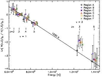
Figure 11.— H₂ level population diagram relative to 1-0S(1) for the six regions of NGC 5135. The data points are slightly spread in the X-direction simply for illustrative purposes. The straight line is the linear fit to the $v=$ 1-0 levels. Its slope is consistent with an isothermal population at $1930\pm 114$ K.

In Fig. 11 the H₂ population diagram for our six regions is presented, showing the column densities normalised by the (1,3) transition versus the energy of the upper level (in Kelvin). We have used six different emission lines including four $v=$ 1-0 transitions (S(0), S(1), S(2) and S(3)) and two $v=$ 2-1 transitions (S(1) and S(3)). The different symbols represent our six regions of integrated spectra.

The $v=$ 1-0 transitions are clearly well thermalized in all regions, consistent with a similar thermal excitation temperature. By a linear least square minimisation to the $v=$ 1-0 transitions, we have found a common excitation temperature of $1930\pm 114$ K which is in agreement with the temperature range $2000-3000$ K derived from Fig. 10. The reason for using only the $v=$ 1-0 lines for the fit resides in that these lower energy transitions are mainly susceptible to thermal processes, while higher energy transitions ($v=$ 2-1) are more easily affected by fluorescence and other non-thermal mechanisms (if present).

For the $v=$ 2-1 transitions, however, the situation looks dissimilar. While the (2,5) transitions are consistent with the thermal linear fit, the (2,3) ones are shifted upwards this relation. The exception is region A for which all transitions are consistent with a thermal mechanism. The (2,3) deviation of the remaining areas could be explained by some contribution from UV-fluorescence, expected to be present in starforming regions. However, when fluorescence dominates the H₂ excitation, a larger positive offset between the 2-1 transitions and our fit would be expected, with line ratios like 2-1S(1)/1-0S(1) of about 0.5. The observed values in Fig. 10 are rather smaller ($<\,0.2$), suggesting that UV-fluorescence might be present but does not dominates the H₂ excitation. The (2,5) transition case is rather different, with larger uncertainties in the data. However we just point out that almost all data points lie very close to the thermal linear fit, which is not expected for $v=$ 2-1 transitions if fluorescence is present. As mentioned in Sec. 3.5.1, the Draine & Woods (1990) X-ray models predict a (2,5) transition decrement which may explain the observed behaviour but, in principle, only for regions A and E (the only two with clear X-ray sources). The existence of a second thermal component for the $v=$ 2-1 transitions cannot be explored given the uncertainties.

3.6. [FeII] as a SNe tracer

For many years different authors have suggested that the [FeII]-emission from galaxies traces the fast shocks produced by SNR and so, their SNe activity (e.g. Graham et al. 1987, Moorwood & Oliva 1988, Oliva et al. 1989, Greenhouse et al. 1991, Colina 1993, Alonso-Herrero et al. 2003, Labrie & Pritchet 2006). The partial ISM ionization produced by this mechanism is suitable for most of the Fe atoms to be in low ionization states.

Different authors have derived empirical correlations we can use to estimate the SNe rate directly from the [FeII] data. Calzetti (1997) has found the following expression for [FeII] measurements

$$SN_{rate,Ca97}(yr^{-1})=5.38\cdot L_{[FeII]}(W)\times 10^{-35},$$ (5)

for which SNes release $\rm 10^{51}\,erg$ of energy during their lives. Also, from their study of SNR in M82 and NGC 253, Alonso-Herrero et al. (2003) have found that

$$SN_{rate,AH03}(yr^{-1})=8.0\cdot L_{[FeII]}(W)\times 10^{-35}.$$ (6)

In Table 5 we present the derived SNe rates for regions B-F by using eqs. 5-6. Region A has been excluded from the analysis because it is likely that the [FeII]-emission comes from the AGN and not from SNe.

Table 5SNe Rates derived from [FeII] emission

Reg	Ca97	A-H03
	$\rm[yr^{-1}]$	$\rm[yr^{-1}]$
Bb	0.006 $\pm$ 0.001	0.009 $\pm$ 0.002
Cb	0.006 $\pm$ 0.001	0.009 $\pm$ 0.002
Db	0.011 $\pm$ 0.002	0.017 $\pm$ 0.004
Eb	0.027 $\pm$ 0.006	0.041 $\pm$ 0.009
Fb	0.006 $\pm$ 0.001	0.009 $\pm$ 0.002
Tot. -Aa,b	0.368 $\pm$ 0.084	0.547 $\pm$ 0.125

(^a) The complete H-band FoV was collapsed in a single spectrum and the measured [FeII] flux was extinction corrected by our median FoV-extinction value of $A_{V}=6\rm\,mag$. For this calculation, the [FeII] flux from region A has been subtracted from the total because it likely comes from the AGN and not from SNe. (^b) Our extinction corrected [FeII] fluxes were used. For B-F it corresponds to apertures of 157 pc in diameter.

We remind the reader that all SNe rates derived from [FeII] are upper limits because we are assuming that all [FeII] flux comes from SNR. We have already seen in previous sections that there exist other processes that might contribute to [FeII] enhancement.

The total-FoV SNe rate from Table 5 is rather high compared to other well studied starburst galaxies. The rates derived for the entire galaxies M82 and NGC 253 by Alonso-Hererro et al. (2003) of $\rm\approx 0.1\,yr^{-1}$ are about 5$\,\times$ lower than our [FeII] estimation between the central $\rm 2.3\,kpc\times 2.3\,kpc$ of NGC 5135. The source of this discrepancy is the different SFRs of these galaxies. By using Sanders et al. (2003) IRAS data and the Kennicutt (1998) law, we estimate total SFRs of 15.0, 3.4 and $\rm 7.0\,M_{\odot}yr^{-1}$ for NGC 5135, NGC 253 and M82, respectively. For NGC 5135, we subtract the AGN contribution (25%, Alonso-Herrero et al. 2006b) from the total far-IR luminosity used in this calculation. As we can see, the different SNe rates between NGC 5135 and NGC 253 can be explained by the stronger SFR of the former. The relative SFRs of NGC 5135 and M82 can also explain their different SNe rates between a factor of 2. Such a difference can be easily attributed to the many uncertainties of this calculation, including the flux measurements, the presence of different alternative sources for those fluxes and the implicit models assumptions for the SNe rates and SFRs determination.

Forbes & Ward (1993) have found a tight correlation between the 6 cm and [FeII]-emission and it is also well known that SNe and SNR shells are strong radio emitters. Therefore, to first order, a spatial correspondence between radio and [FeII]-emission could be expected. To test this, in Fig. 12 we compare our [FeII] flux map with VLA $\rm 6\,cm$ radio emission (contours, $\rm 0.91^{\prime\prime}\times 0.60^{\prime\prime}$ beam resolution) obtained by Ulvestad & Wilson (1989). Both images were aligned by matching the corresponding nuclear (A region) unresolved peak. As we can see, the spatial structures are in good agreement, suggesting that at least part of the [FeII]-emission comes from SNRs.

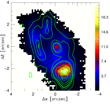
Figure 12.— [FeII] flux map. The contours are the $\rm 6\,cm$ VLA radio emission from Ulvestad & Wilson (1989).

We can go further on our comparison by contrasting the SNe rates derived from radio and [FeII]-emission in our B-F regions. To do so, however, we have the limitation of the poorer spatial resolution of the 6 cm VLA image. Therefore, we decided to keep the centers of our B-F regions but use a larger circular aperture of $\rm 0.91^{\prime\prime}$ ($\rm\approx 260\,pc$ in diameter, the larger dimension of the radio beam size). We label our $\rm 0.91^{\prime\prime}$ aperture regions as B^′-F^′. In this way, both our [FeII] and 6 cm emission were remeasured within the new apertures. We highlight that, for this larger aperture, regions D^′ and E^′ share about 40 $\%$ of their spaxels.

In a similar way to [FeII], other works have explored the relation between the 6 cm radio flux and the SNe rate. By using models and empirical correlations, the different authors have made diverse assumptions concerning the origin of their radio observations. From their study of compact radio sources in M82, Huang et al. (1994) derived the following expression

$$SN_{rate,Hu94}^{6\rm cm}(yr^{-1})=0.22\cdot L_{\nu}(W\,Hz^{-1})\times 10^{-22}.$$ (7)

These authors assume that the entire non-thermal radio emission of M82 comes from SNRs. $L_{\nu}$ is the 6 cm radio flux in [$\rm W\,Hz^{-1}$].

In a study of the brightest radio sources in Arp 299, Neff et al. (2004) derived a similar expression for the SNe rate as a function of the 6 cm radio flux from SNRs

$$SN_{rate,Ne04}^{6\rm cm}(yr^{-1})=$$

$$\frac{0.37\cdot f\cdot L_{\nu}(W\,Hz^{-1})\cdot 10^{33}}{5\,{\rm mJy}\cdot 4\pi(D_{Arp299})^{2}}\times\bigg{(}\frac{408}{4885}\bigg{)}^{\alpha+0.75}$$ (8)

According to the authors, this equation is valid for few hundred parsec spatial scales, the same order of our own aperture diameters. Eq. 8 has been modified to adapt the measured radio flux in NGC 5135 to the distance of Arp 299 ($\approx$ 42 Mpc, for which the original expression was made). The spectral index $\alpha$ was chosen to be $-0.58$, a value consistent with typical Galactic SNRs (Weiler et al. 2002) and with the Neff et al. measurements in Arp 299. The parameter $f$ is the fraction of radio flux density that can be associated with individual SNRs on parsec scales. Because there exist other sources of radio emission apart of SNR, we adopt a $f$ value of 0.15 following Neff et al. An $f$ value of 0.1-0.2 provides a calibration similar to those obtained by Condon (1992) and Huang et al. (1994) works on radio sources in starburst galaxies. Also, the chosen value of $f$ is in excellent agreement with Colina & Pérez-Olea (1995) models: for the majority of them the fraction of SNR radio emission with respect to other sources (free-free emission, young radio SNe) ranges between 9-19% of the total flux.

Finally, we have also used Pérez-Olea & Colina (1995) model predictions for the SNe rate, based on our $6\rm cm$ measurements and Br$\gamma$ age estimations. An instantaneous burst and Salpeter IMF have been assumed, and different masses M_up (30, 60, 1200$\,\rm M_{\odot}$) and M_low (0.85, 3$\,\rm M_{\odot}$) have been considered for the calculations. These models make a detailed consideration of the different radio components, including free-free radiation, young radio SNe and older SNRs. In Table 6 we present the SNe rates derived from [FeII] and 6 cm radio emission (eqs. 5-8) for regions B^′-F^′.

Table 6SNe Rates derived from [FeII] and Radio emission

Rega	Ca97[FeII]	A-H03[FeII]	Hu946cm	Ne046cm	P-O95${}_{\rm 6cm}^{b}$
	$\rm[yr^{-1}]$	$\rm[yr^{-1}]$	$\rm[yr^{-1}]$	$\rm[yr^{-1}]$	$\rm[yr^{-1}]$
B′	0.012 $\pm$ 0.002	0.017 $\pm$ 0.004	0.012 $\pm$ 0.004	0.019 $\pm$ 0.007	0.013-0.014
C′	0.012 $\pm$ 0.003	0.018 $\pm$ 0.004	0.010 $\pm$ 0.005	0.016 $\pm$ 0.008	0.011-0.012
D′	0.024 $\pm$ 0.005	0.036 $\pm$ 0.008	0.032 $\pm$ 0.075	0.051 $\pm$ 0.118	0.036-0.037
E′	0.051 $\pm$ 0.012	0.076 $\pm$ 0.016	0.064 $\pm$ 0.001	0.100 $\pm$ 0.002	0.071-0.074
F′	0.011 $\pm$ 0.002	0.016 $\pm$ 0.004	0.012 $\pm$ 0.004	0.019 $\pm$ 0.006	0.018-0.019

(^a) Same centers as B-F regions with aperture of $\rm 0.91^{\prime\prime}$. (^b) For Pérez-Olea & Colina (1995) models, we present ranges of SNe rates for each region, where different upper- and lower-limit masses have been considered for a Salpeter IMF.

Table 6 clearly shows the excellent agreement between [FeII] and radio SNe rate predictions for these $\rm\sim 200\,pc$-scale regions. This agreement is totally independent of the correlation or model used to estimate the SNe rate. These results provide additional support to previous findings in normal starburst galaxies like M82 and NGC 253 where similar SNe rates are predicted from [FeII] and $\rm 6\,cm$ radio emission. The radio predictions in this table are of the same order as those of the brightest radio region in Arp 299 ($0.5$-$1.0\,\rm yr^{-1}$, Neff et al. 2004), a bright IR luminous galaxy.

4. Summary

In this paper we have studied the central $\rm 2.3\,kpc$ of NGC 5135, a nearby LIRG galaxy. By using new NIR IFU spectroscopy (VLT/SINFONI) we have traced different structural components including the coronal gas (an AGN-activity tracer), ionized (young stellar population) and partially ionized gas (SNe remnants), warm molecular gas and the giant/supergiant stellar population. We have selected individual regions of interest for a detailed analysis (see Fig. 3 top panels, and Fig. 4 top-left panel, for their spatial identification). By using these data, we have shown the potential of the IFS technic when applied to a prototype LIRG: studying the complex spatial structure of its different components, the different gas ionization/excitation mechanisms, the AGN activity, the SNe rates, the internal gas/dust extinction and the stellar population ages. Our conclusions are:

1) Overall, we have found that SNR shocks play a dominant role on ionizing/exciting the different gas phases in the central $\rm 2.3\,kpc$ of NGC 5135. Our NIR data reveals that other processes associated to recent star formation and AGN activity usually have a rather localised and smaller overall impact. By using Br$\gamma$-emission, we estimate the AGN contribution to the gas ionization in $\lesssim 3\%$ of the total within our FoV. In the same area, the AGN contributes in $\lesssim 3$-$5\%$ to the total NIR luminosity.

2) We have found the largest ($\rm\sim 600\,pc$ in projection) [SiVI]-ionization cone reported in literature until now. This structure is at least $4\times$ larger than any previous detection in active galaxies. Pointing in opposite direction, a fainter counter-[SiVI]-cone has been also detected.

3) The SNe rates derived from the [FeII] emission are in excellent agreement with $\rm 6\,cm$ radio emission predictions, reinforcing the use of [FeII] as a SNe activity tracer. Typical rates between $0.01$-$\rm 0.04\,yr^{-1}$ were found for individual $\rm\sim 200\,pc$ regions. The [FeII] prediction for our entire FoV ($0.4$-$0.5\rm\,yr^{-1}$) is rather high compared to other starburst galaxies. Such a difference, however, can be explained by the higher SFR of NGC 5135.

4) In a complex spatial distribution, different processes drive the gas ionization depending on the region of interest. These include photoionization from starforming knots (H ii regions B, C and D), SNe remnant shocks (E and F) and AGN photoionization (region A). Mechanisms like stellar X-rays photoionization and star formation might also be present in other regions (E and A, respectively).

5) The molecular gas excitation mechanisms are mainly thermal ($\rm\sim 1930\pm 114\,K$) in all galaxy regions, being X-rays and SNe remnant shocks the dominant processes. Contrary to the expectations we might have for a galaxy with recent star formation, UV-processes like fluorescence have, at the most, a rather marginal contribution even in H ii regions (B, C and D). The column densities found ($\rm N_{H}\sim 10^{21}$-$\rm 10^{22}\,cm^{-2}$) are consistent with previous literature estimations at other wavelengths.

6) As upper limit estimations, the last burst of star formation occurs about $\rm 6$-$\rm 8\,Myr$ ago in all regions, consistent with previous findings in the UV/optical. The presence of a second, older stellar population dominated by bright red giant/supergiant stars is strongly suggested by the data. Although NIR-continuum, CO$\lambda 2.29\mu$m and NaI$\lambda 2.21\mu$m observations agree with this idea, the simple stellar population models cannot clearly discriminate between both populations.

7) For the nucleus (region A), the presence of deep CO$\lambda 2.29\mu$m and NaI$\lambda 2.21\mu$m features highlight the importance of star formation in the AGN neighbourhood ($\rm\leq 90\,pc$ from the center). This is also consistent with previous findings in X-rays.

8) A mean internal visual extinction of $A_{V}=\rm 6\,mag$ ($\rm\approx 0.55\,mag$ at 2.2 $\mu$m) has been measured in the central $\rm 2.3\,kpc$ of this galaxy. For the nucleus (region A) a higher mean value of $A_{V}=\rm 10\,mag$ was found, with a peak of $\rm 17\,mag$ in the very center of this area. This result is qualitatively consistent with high extinctions reported for this region in the literature.

Table 7Fluxes, FWHM and EW for six regions in NGC 5135

		Region A	$\langle A_{V}\rangle=9.71\pm 1.34$			Region B	$\langle A_{V}\rangle=5.11\pm 1.29$
Line	$\lambda_{c}$	Flux	Corr.Flux	FWHM	EW	Flux	Corr.Flux	FWHM	EW
	$\rm[\mu m]$	$[\rm erg\,\,s^{-1}\,cm^{-2}]\times 10^{-16}$	$[\rm erg\,\,s^{-1}\,cm^{-2}]\times 10^{-16}$	[$\rm\AA$]	[$\rm\AA$]	$[\rm erg\,\,s^{-1}\,cm^{-2}]\times 10^{-16}$	$[\rm erg\,\,s^{-1}\,cm^{-2}]\times 10^{-16}$	[$\rm\AA$]	[$\rm\AA$]
1-0 S(0)	2.22	2.69 $\pm$ 0.50	7.20 $\pm$ 1.67	14.41 $\pm$ 2.09	2.08 $\pm$ 0.39	0.86 $\pm$ 0.20	1.44 $\pm$ 0.38	8.70 $\pm$ 1.48	2.47 $\pm$ 0.57
1-0 S(1)	2.12	11.66 $\pm$ 0.51	33.62 $\pm$ 5.14	13.06 $\pm$ 0.41	9.28 $\pm$ 0.40	3.07 $\pm$ 0.25	5.36 $\pm$ 0.87	10.64 $\pm$ 0.61	8.54 $\pm$ 0.69
1-0 S(2)	2.03	4.19 $\pm$ 0.52	12.97 $\pm$ 2.60	14.11 $\pm$ 1.30	3.34 $\pm$ 0.42	1.20 $\pm$ 0.27	2.17 $\pm$ 0.59	12.33 $\pm$ 2.09	3.10 $\pm$ 0.71
1-0 S(3)	1.96	13.22 $\pm$ 0.56	43.86 $\pm$ 7.51	15.03 $\pm$ 0.46	10.64 $\pm$ 0.45	2.98 $\pm$ 0.28	5.60 $\pm$ 1.04	12.22 $\pm$ 0.84	7.25 $\pm$ 0.68
2-1 S(1)	2.25	1.16 $\pm$ 0.37	3.05 $\pm$ 1.06	9.19 $\pm$ 2.20	0.90 $\pm$ 0.29	0.60 $\pm$ 0.20	0.99 $\pm$ 0.36	9.83 $\pm$ 2.47	1.77 $\pm$ 0.60
2-1 S(3)	2.07	1.03 $\pm$ 0.41	3.08 $\pm$ 1.31	11.04 $\pm$ 3.30	0.81 $\pm$ 0.32	0.47 $\pm$ 0.21	0.84 $\pm$ 0.40	9.55 $\pm$ 3.23	1.24 $\pm$ 0.56
Br$\gamma$	2.16	5.18 $\pm$ 0.57	14.46 $\pm$ 2.60	21.48 $\pm$ 1.76	4.05 $\pm$ 0.45	7.26 $\pm$ 0.29	12.45 $\pm$ 1.77	12.00 $\pm$ 0.33	20.54 $\pm$ 0.83
Br$\delta$	1.94	2.65 $\pm$ 0.51	8.89 $\pm$ 2.27	11.85 $\pm$ 1.68	2.11 $\pm$ 0.41	3.94 $\pm$ 0.32	7.44 $\pm$ 1.34	9.91 $\pm$ 0.56	9.42 $\pm$ 0.76
$\rm[SiVI]$	1.96	26.83 $\pm$ 0.80	88.53 $\pm$14.86	27.95 $\pm$ 0.59	20.78 $\pm$ 0.62	— —	— —	— —	— —
$\rm[FeII]$	1.64	17.04 $\pm$ 1.20	82.30 $\pm$18.86	15.76 $\pm$ 0.81	6.49 $\pm$ 0.46	11.54 $\pm$ 0.71	26.44 $\pm$ 5.76	10.16 $\pm$ 0.44	10.48 $\pm$ 0.64
HeI	2.06	2.74 $\pm$ 0.49	8.30 $\pm$ 1.96	14.83 $\pm$ 1.98	2.16 $\pm$ 0.39	1.94 $\pm$ 0.26	3.48 $\pm$ 0.69	11.70 $\pm$ 1.13	5.08 $\pm$ 0.67
CO	2.29	6.76 $\pm$ 0.18	7.37 $\pm$ 1.61	— —	2.15 $\pm$ 0.06	3.96 $\pm$ 0.23	4.31 $\pm$ 0.97	— —	4.98 $\pm$ 0.29
NaI	2.21	2.36 $\pm$ 0.06	2.60 $\pm$ 0.57	— —	0.79 $\pm$ 0.02	1.01 $\pm$ 0.05	1.12 $\pm$ 0.25	— —	1.35 $\pm$ 0.07
		Region C	$\langle A_{V}\rangle=5.93\pm 1.29$			Region D	$\langle A_{V}\rangle=3.99\pm 1.29$
1-0 S(0)	2.22	0.68 $\pm$ 0.22	1.23 $\pm$ 0.43	8.85 $\pm$ 2.12	1.52 $\pm$ 0.49	1.21 $\pm$ 0.23	1.82 $\pm$ 0.42	14.18 $\pm$ 2.02	4.87 $\pm$ 0.92
1-0 S(1)	2.12	2.71 $\pm$ 0.27	5.17 $\pm$ 0.90	10.48 $\pm$ 0.76	5.65 $\pm$ 0.57	4.99 $\pm$ 0.27	7.71 $\pm$ 1.16	15.43 $\pm$ 0.58	20.82 $\pm$ 1.12
1-0 S(2)	2.03	1.42 $\pm$ 0.36	2.82 $\pm$ 0.84	16.46 $\pm$ 3.16	2.66 $\pm$ 0.68	1.76 $\pm$ 0.28	2.80 $\pm$ 0.61	17.02 $\pm$ 1.97	6.56 $\pm$ 1.04
1-0 S(3)	1.96	3.07 $\pm$ 0.34	6.39 $\pm$ 1.24	13.58 $\pm$ 1.10	5.29 $\pm$ 0.58	4.99 $\pm$ 0.31	8.16 $\pm$ 1.39	16.80 $\pm$ 0.74	16.51 $\pm$ 1.02
2-1 S(1)	2.25	0.56 $\pm$ 0.25	1.01 $\pm$ 0.47	11.67 $\pm$ 3.96	1.32 $\pm$ 0.58	0.90 $\pm$ 0.23	1.34 $\pm$ 0.38	15.47 $\pm$ 2.98	3.75 $\pm$ 0.94
2-1 S(3)	2.07	0.28 $\pm$ 0.23	0.54 $\pm$ 0.45	8.54 $\pm$ 5.23	0.54 $\pm$ 0.44	0.50 $\pm$ 0.19	0.78 $\pm$ 0.33	11.38 $\pm$ 3.30	1.88 $\pm$ 0.73
Br$\gamma$	2.16	6.17 $\pm$ 0.31	11.55 $\pm$ 1.68	12.20 $\pm$ 0.43	13.31 $\pm$ 0.68	5.21 $\pm$ 0.26	7.94 $\pm$ 1.15	14.12 $\pm$ 0.49	21.17 $\pm$ 1.06
Br$\delta$	1.94	3.14 $\pm$ 0.35	6.58 $\pm$ 1.29	10.18 $\pm$ 0.82	5.31 $\pm$ 0.59	2.92 $\pm$ 0.29	4.81 $\pm$ 0.91	11.83 $\pm$ 0.83	9.28 $\pm$ 0.93
$\rm[SiVI]$	1.96	— —	— —	— —	— —	— —	— —	— —	— —
$\rm[FeII]$	1.64	11.00 $\pm$ 0.84	28.78 $\pm$ 6.40	10.97 $\pm$ 0.60	6.64 $\pm$ 0.51	27.40 $\pm$ 1.05	52.33 $\pm$11.12	28.74 $\pm$ 0.79	40.94 $\pm$ 1.57
HeI	2.06	1.81 $\pm$ 0.29	3.56 $\pm$ 0.78	11.83 $\pm$ 1.42	3.44 $\pm$ 0.56	1.72 $\pm$ 0.24	2.71 $\pm$ 0.55	14.92 $\pm$ 1.55	6.35 $\pm$ 0.90
CO	2.29	5.86 $\pm$ 0.31	6.39 $\pm$ 1.43	— —	5.93 $\pm$ 0.31	3.03 $\pm$ 0.21	3.31 $\pm$ 0.76	— —	5.46 $\pm$ 0.38
NaI	2.21	1.66 $\pm$ 0.07	1.83 $\pm$ 0.41	— —	1.56 $\pm$ 0.07	0.93 $\pm$ 0.05	1.03 $\pm$ 0.23	— —	1.64 $\pm$ 0.1
		Region E	$\langle A_{V}\rangle=4.75\pm 1.29$			Region F	$\langle A_{V}\rangle=5.61\pm 1.34$
1-0 S(0)	2.22	1.49 $\pm$ 0.29	2.41 $\pm$ 0.57	13.76 $\pm$ 2.06	3.59 $\pm$ 0.70	0.66 $\pm$ 0.16	1.16 $\pm$ 0.32	10.54 $\pm$ 1.83	3.78 $\pm$ 0.89
1-0 S(1)	2.12	7.68 $\pm$ 0.36	12.89 $\pm$ 1.91	18.47 $\pm$ 0.62	19.04 $\pm$ 0.91	2.62 $\pm$ 0.20	4.84 $\pm$ 0.80	12.20 $\pm$ 0.66	13.86 $\pm$ 1.08
1-0 S(2)	2.03	3.20 $\pm$ 0.40	5.56 $\pm$ 1.09	21.30 $\pm$ 1.96	7.05 $\pm$ 0.88	1.10 $\pm$ 0.23	2.12 $\pm$ 0.55	14.43 $\pm$ 2.17	5.15 $\pm$ 1.06
1-0 S(3)	1.96	8.87 $\pm$ 0.42	15.96 $\pm$ 2.65	18.42 $\pm$ 0.63	17.48 $\pm$ 0.83	2.80 $\pm$ 0.23	5.60 $\pm$ 1.04	13.31 $\pm$ 0.79	12.10 $\pm$ 1.01
2-1 S(1)	2.25	1.38 $\pm$ 0.45	2.22 $\pm$ 0.78	24.00 $\pm$ 6.61	3.48 $\pm$ 1.13	0.39 $\pm$ 0.13	0.69 $\pm$ 0.25	8.68 $\pm$ 2.18	2.37 $\pm$ 0.81
2-1 S(3)	2.07	0.71 $\pm$ 0.28	1.21 $\pm$ 0.51	13.89 $\pm$ 4.12	1.56 $\pm$ 0.62	0.29 $\pm$ 0.15	0.55 $\pm$ 0.29	8.83 $\pm$ 3.29	1.43 $\pm$ 0.73
Br$\gamma$	2.16	4.07 $\pm$ 0.30	6.72 $\pm$ 1.04	14.23 $\pm$ 0.74	9.87 $\pm$ 0.72	1.86 $\pm$ 0.19	3.36 $\pm$ 0.59	13.52 $\pm$ 1.00	10.26 $\pm$ 1.06
Br$\delta$	1.94	2.17 $\pm$ 0.32	3.92 $\pm$ 0.86	10.28 $\pm$ 1.12	4.09 $\pm$ 0.61	1.14 $\pm$ 0.22	2.30 $\pm$ 0.59	10.19 $\pm$ 1.41	4.81 $\pm$ 0.93
$\rm[SiVI]$	1.96	— —	— —	— —	— —	0.51 $\pm$ 0.20	1.02 $\pm$ 0.43	11.42 $\pm$ 3.23	2.11 $\pm$ 0.81
$\rm[FeII]$	1.64	57.34 $\pm$ 1.58	123.91 $\pm$26.12	33.54 $\pm$ 0.68	50.59 $\pm$ 1.39	10.50 $\pm$ 0.72	26.10 $\pm$ 5.96	18.03 $\pm$ 0.88	15.20 $\pm$ 1.04
HeI	2.06	1.40 $\pm$ 0.30	2.41 $\pm$ 0.62	14.45 $\pm$ 2.28	3.06 $\pm$ 0.65	0.68 $\pm$ 0.18	1.28 $\pm$ 0.40	11.90 $\pm$ 2.41	3.23 $\pm$ 0.88
CO	2.29	6.46 $\pm$ 0.37	7.04 $\pm$ 1.58	— —	7.00 $\pm$ 0.40	1.66 $\pm$ 0.14	1.82 $\pm$ 0.42	— —	4.44 $\pm$ 0.37
NaI	2.21	1.93 $\pm$ 0.09	2.13 $\pm$ 0.47	— —	2.01 $\pm$ 0.09	0.60 $\pm$ 0.04	0.66 $\pm$ 0.15	— —	1.51 $\pm$ 0.10

References

- (1) Alonso-Herrero, A., Rieke, M. J., Rieke, G. H., Ruiz, M., 1997, ApJ, 482, 747
- (2) Alonso-Herrero, A., Rieke, M. J., Rieke, G. H., Kelly, D. M., 2001, Ap&SS, 276, 1109
- (3) Alonso-Herrero, A., Rieke, G. H., Rieke, M. J., Kelly, D. M., 2003, AJ, 125, 1210
- (4) Alonso-Herrero, A., Rieke, G. H., Rieke, M. J., Colina, L., Pérez-González, P. G., Ryder, S. D., 2006a, ApJ, 650, 835
- (5) Alonso-Herrero, A., Colina, L., Packham, Ch., Díaz-Santos, T., Rieke, G. H., Radomski, J. T., Telesco, Ch. M., 2006b, ApJ, 652, 83
- (6) Alonso-Herrero, A. et al. 2009, arXiv0903.1495
- (7) Arribas, S., Bushouse, H., Lucas, R. A., Colina, L., Borne, K. D., 2004, AJ, 127, 2522
- (8) Arribas, S., Colina, L., Monreal-Ibero, A., Alfonso, J., García-Marín, M., Alonso-Herrero, A., 2008, A&A, 479, 687
- (9) Black, J. H., van Dishoeck, E. F., 1987, ApJ, 322, 412
- (10) Blain, A. W., Smail, I., Ivison, R. J., Kneib, J.-P., Frayer, D. T., 2002, PhR, 369, 111
- (11) Bonnet, H. et al. 2004, The ESO Messenger, 117, 17
- (12) Brand, P. W. J. L., Toner, M. P., Geballe, T. R., Webster, A. S., Williams, P. M., Burton, M. G., 1989, MNRAS, 236, 929
- (13) Burston, A. J., Ward, M. J., Davies, R. I., 2001, MNRAS, 326, 403
- (14) Bushouse, H. A. et al. 2002, ApJS, 138, 1
- (15) Calzetti, D., Armus, L., Koornneef, J., Storchi-Bergmann, T., ApJ, 533, 682
- (16) Calzetti, D., 1997, AJ, 113, 1
- (17) Caputi, K. I., Lagache, G., Yan, L., Dole, H., Bavouzet, N., Le Floc’h, E., Choi, P. I., Helou, G., Reddy, N., 2007, ApJ, 660, 97
- (18) Chapman, S. C., Windhorst, R., Odewahn, S., Yan, H., Conselice, C., 2003, ApJ, 599, 92
- (19) Chiosi, C., Bertelli, G., Bressan, A., Nasi, E., 1986, A&A, 165, 84
- (20) Cid Fernandes, R. et al. 2004, ApJ, 605, 105
- (21) Clavel, J., Wamsteker, W., Glass, I. S., 1989, ApJ, 337, 236
- (22) Clavel, J. et al. 1992, ApJ, 393, 113
- (23) Colina, L., 1993, ApJ, 411, 565
- (24) Colina, L., Pérez-Olea, D. E., 1995, 1995, MNRAS, 277, 845
- (25) Colina, L., Arribas, S. & Monreal-Ibero, A., 2005, ApJ, 621, 725
- (26) Condon, J. J., 1992, ARA&A, 30, 575
- (27) Contini, m., Prieto, M. A., & Viegas, S. M., 1998, ApJ, 505, 621
- (28) Dasyra, K. M. et al. 2006, ApJ, 651, 835
- (29) Davies, R. I., Sugai, H., Ward, M. J., 1997, MNRAS, 291, 314
- (30) Davies, R. I., Sternberg, A., Lehnert, M., Tacconi-Garman, L. E., 2003, ApJ, 597, 907
- (31) Davies, R. I., Sternberg, A., Lehnert, M. D., Tacconi-Garman, L. E., 2005, ApJ, 633, 105
- (32) Davies, R. I., Mueller Sánchez, F., Genzel, R., Tacconi, L. J., Hicks, E. K. S., Friedrich, S., Sternbrg, A., 2007, ApJ, 671, 1388
- (33) Díaz-Santos, T., Alonso-Herrero, A., Colina, L., Packham, Ch., Radomski, J. T., Telesco, Ch. M., 2008, ApJ, 685, 211
- (34) Doherty, R. M., Puxley, P. J., Lumsden, S. L., Doyon, R., 1995, MNRAS, 277, 577
- (35) Draine, B. T., Woods, D. T., 1990, ApJ, 363, 464
- (36) Draine, B. T., Woods, D. T., 1991, ApJ, 383, 621
- (37) Egami, E. et al. 2004, ApJS, 154, 130
- (38) Eisenhauer, F. et al. 2003, SPIE, 4841, 1548
- (39) Ferguson, J. W., Korista, K. T. & Ferland, G. J., 1997, ApJS, 110, 287
- (40) Forbes, D. A., Ward, M. J., Depoy, D. L., Boisson, C., Smith, M. S., 1992, MNRAS, 254, 509
- (41) Forbes, D. A., Ward, M. J., 1993, ApJ, 416, 150
- (42) Frster Schreiber, N. M., 2000, AJ, 120, 2089
- (43) Frayer, D. T., Armus, L., Scoville, N. Z., Blain, A. W., Reddy, N. A., Ivison, R. J., Smail, I., 2003, AJ, 126, 73
- (44) García-Barreto, J. A., Franco, J., Carrillo, R., Venegas, S., Escalante-Ramìrez, B., 1996, RMxAA, 32, 89
- (45) Gardner, J. P., et al. , 2006, SSRv, 123, 485
- (46) Genzel, R., et al. , 1998, ApJ, 498, 579
- (47) Genzel, R., Tacconi, L. J., Rigopoulou, D., Lutz, D., Tecza, M., 2001, ApJ, 563, 527
- (48) Glass, I. S., 1992, MNRAS, 256, 23
- (49) Graham, J. R., Wright, G. S., Longmore, A. J., 1987, ApJ, 313, 847
- (50) Greenhouse, M. A., Woodward, Ch. E., Thronson, H. A. Jr., Rudy, R. J., Rossano, G. S., Erwin, P., Puetter, R. C., 1991, ApJ, 383, 164
- (51) González Delgado, R. M., Heckman, T., Leitherer, C., Meurer, G., Krolik, J., Wilson, A. S., Kinney, A., Koratkar, A., 1998, ApJ, 505, 174
- (52) Graham, J. R., Wright, G. S., Longmore, A. J., 1987, ApJ, 313, 847G
- (53) Haniff, C. A., Wilson, A. S., Ward, M., 1988, ApJ, 334, 104
- (54) Heckman, T. M., Armus, L., Miley, G. K., 1990, ApJS, 74, 833
- (55) Huang, Z. P., Thuan, T. X., Chevalier, R. A., Condon, J. J., Yin, Q. F., 1994, ApJ, 424, 114
- (56) Huchra,J. P., 1983, unpublished list of active galaxies
- (57) Huchra,J. P., Davis, M., Latham, D., Tonry, J., 1983, ApJS, 52, 89
- (58) Kawara, K., Taniguchi, Y., Nishida, M., 1988, ApJ, 328, 41
- (59) Kennicutt, R. C., 1998, ApJ, 498, 541
- (60) Kinney, A. L., Bohlin,R. C., Calzetti, D., Panagia, N., Wyse, R. F. G., 1993, APJS, 86, 5
- (61) Kleinmann G., Hall D. N. B., 1986, ApJS, 62, 501
- (62) Kleinmann, D. E. & Low, F. J., 1970, ApJ, 159, 165
- (63) Kollatschny, W. & Fricke, K. J., 1989, A&A, 219, 34
- (64) Labrie, K. & Pritchet, C. J., 2006, ApJS, 166, 188
- (65) Le Floch, E. et al. 2004, ApJS, 154, 170L
- (66) Le Floch, E. et al. 2005, ApJ, 632, 169
- (67) Leitherer, C. et al. , 1999, ApJS, 123, 3
- (68) Johnson]JJ07 Levenson, N. A., Weaver, K. A., Heckman, T. M., Awaki, H., Terashima, Y., ApJ, 2004, 602, 135
- (69) Lumsden, S. L., Puxley, P. J., Hoare, M. G., 2001, MNRAS, 320, 83
- (70) Maiolino, R., Alonso-Herrero, A., Anders, S., Quillen, A., Rieke, M. J., Rieke, G. H., Tacconi-Garman, L. E., 2000, ApJ, 531, 219
- (71) Maloney, P. R., Hollenbach, D. J., Tielens, A., 1996, ApJ, 466, 561
- (72) Marco, O., Alloin, D., 1998, A&A, 336, 823
- (73) Marco, O., Alloin, D., 2000, A&A, 353, 465
- (74) Marconi, A., Moorwood, A. F. M., Salvati, M., Oliva, E.,1994, A&A, 291,18
- (75) Monreal-Ibero, A., Arribas, S., Colina, L., 2006, ApJ, 637, 138
- (76) Moorwood, A. F. & Oliva E., 1988, A&A 203, 278
- (77) Mouri, H., Nishida, M., Taniguchi, Y., Kawara, K., 1990, ApJ, 360, 55
- (78) Mouri, H., 1994, ApJ, 427, 777
- (79) Mouri H., Kawara, K., Taniguchi, Y., 2000, ApJ, 528, 186
- (80) Mulchaey, J., Reagan, M. W., Kundu, A., 1997, ApJS, 110, 299
- (81) Neff, S. G., Ulvestad, J. S., Teng, S. H., 2004, ApJ, 611, 186
- (82) Oliva, E., Moorwood, A. F. M., Danziger, I. J., 1989, A&A, 214, 307
- (83) Oliva, E., Moorwood, A. F. M., Danzier, I. J., 1990, A&A, 240, 453
- (84) Origlia, L. & Oliva, E., 2000, A&A, 357, 61
- (85) Osterbrock, D. E., 1989, Astrophysics of Gaseous Nebulae and Active Galactic Nuclei, University Science Books, Mill Valley, California
- (86) Pérez-González, P. et al. 2005, ApJ, 630, 82
- (87) Pérez-Olea, D. E., Colina, L., 1995, MNRAS, 277, 857
- (88) Perryman, M. A. C., et al. 1997, A&A, 323L, 49
- (89) Pickles, A. J., 1998, PASP, 110, 863
- (90) Phillips, M. M., Charles, P. A., Baldwin, J. A., 1983, ApJ, 266, 485
- (91) Prieto, M. A., Marco, O., Gallimore, J., 2005, MNRAS, 364L, 28
- (92) Quillen, A. C., Alonso-Herrero, A., Rieke, M. J., Rieke, G. H.; Ruiz, M., Kulkarni, V., 1999, ApJ, 527, 696
- (93) Renzini, A., Buzzoni, A., 1986, In: Chiosi, J. G., Renzini, A. (eds.), Spectral Evolution of Galaxies, p. 195
- (94) Rieke, G. H., Low, F. J., 1972, ApJ, 176, L95
- (95) Rodríguez-Ardila, A., Contini, M., Viegas, S. M., 2005a, MNRAS, 357, 220
- (96) Rodríguez-Ardila, A., Pastoriza, M. G., Viegas, S. Sigut, T. A. A., Pradhan, A. K., 2005b, MNRAS, 364, 1041
- (97) Rodríguez-Ardila, A. K., Mazzalay, X., 2006a, MNRAS, 367L, 57
- (98) Rodríguez-Ardila, A. K., Prieto, M. A., Viegas, S., Gruenwald, R., 2006b, ApJ, 653, 1098
- (99) Sanders, D. B., Scoville, N. Z., Soifer, B. T., 1991, ApJ, 370, 158
- (100) Sanders, D. B., Mirabel, I. F., 1996, ARA&A, 34, 749
- (101) Sanders, D. B., Mazzarella, J. M., Kim, D.-C., Surace, J. A., Soifer, B. T., 2003, AJ, 126, 1607
- (102) Schlegel, D. J., Finkbeiner, D. P., Davis, M., 1998, ApJ, 500,525
- (103) Shields J., 1993, ApJ, 419, 181
- (104) Skrutskie, M. F., et al. 2006, AJ, 131, 1163
- (105) Solomon, P. M., Downes, D., Radford, S. J. E., Barrett, J. W., 1997, ApJ, 478, 144
- (106) Spoon, H. W. W., Marshall, J. A., Houck, J. R., Elitzur, M., Hao, L., Armus, L., Brandl, B. R., Charmandaris, V., 2007, ApJ, 654L, 49
- (107) Sternberg, A., 1998, ApJ, 506, 721
- (108) Sternberg, A., Dalgarno, A., 1989, ApJ, 338, 197
- (109) Thornley, M. D., F rster Schreiber, N. M., Lutz, D. Genzel, R., Spoon, H. W. W., Kunze, D., Sternberg, A., 2000, ApJ, 539, 641
- (110) Thuan, A., 1984, ApJ, 281, 126
- (111) Ulvestad, J. S. & Wilson, A. S., 1989, ApJ, 343, 659
- (112) Vanzi, L., Rieke, G. H., Martin, C. L., Shields, J. C., 1996, ApJ, 466, 150
- (113) Viegas-Aldrovandi, S. & Contini, M., 1989, ApJ, 339, 689
- (114) Weaver, K. A., 2001, ASPC, 249, 389
- (115) Weiler, K. W., Panagia, N., Montes, M. J., Sramek, R. A., 2002, ARA&A, 40, 387
- (116) Wolniewicz, L., Simbotin, I., Dalgarno, A., 1998, ApJS, 115, 293
- (117) Zuther, J., Iserlohe, C., Pott, J.-U., Bertram, T., Fischer, S., Voges, W., Hasinger, G., Eckart, A., 2007, A&A, 466, 451