Evaluation of Born and local effective charges in unoriented materials from vibrational spectra

Abstract

We present an application of the Lorentz model in which fits to vibrational spectra or a Kramers Kronig analysis are employed along with several useful formalisms to quantify microscopic charge in unoriented (powdered) materials. The conditions under which these techniques can be employed are discussed, and we analyze the vibrational response of a layered transition metal dichalcogenide and its nanoscale analog to illustrate the utility of this approach.

I Introduction

Born and local (or ionic) effective charge are well-known quantities with which to assess chemical bonding and polarization in a material.Born1918 ; Szigeti1950 A large local effective charge indicates a highly ionic system (for instance, 0.8 in NaCl), a medium-sized value points toward an intermediate bonding case (0.4 in GaAs), and a small value is associated with a covalent material (0 in Si).Ashcroft1976 ; Kittel1966 On the other hand, Born effective charge describes the static and dynamic polarizations.Born1954 From the optical properties point of view, large longitudinal optic-transverse optic (LO-TO) splittings are well-known characteristics of polarizable compounds and associated with substantial Born effective charges. This is because LO-TO splitting is directly proportional to charge within Born’s original formalism.Born1918 Using the LO-TO splitting and high frequency dielectric constant, it is relatively straightforward to quantify chemical bonding from optical measurements of high quality single crystal samples and compare the extracted value(s) with first principles calculations.Lee2003 ; Fontana1984 ; Zhong1994 Unfortunately, there are many instances when single crystals of a bulk material are unavailable, either because they can not be grown or are not of sufficient size or quality for optical measurements. At the same time, nanoparticles, nanotubes, and alloys (or composite mixtures) present scientifically compelling problems, Long2007 ; Tenne2004 ; Poudel2008 ; Hochbaum2008 ; Boukai2008 ; Cao2007 ; Carr1985 where optical measurements on powdered materials are the only option, a drawback that complicates the situation but does not diminish the desirability of obtaining quantitative Born and local effective charge data.

Following Born and Szigeti,Born1918 ; Szigeti1950 we present an application of the Lorentz model in which fits to vibrational spectra or a Kramers Kronig analysis are employed along with several useful formalisms to quantify microscopic charge in unoriented (powdered) materials, assuming that the effects of ionic displacement and atomic polarizability are superimposable. We demonstrate that this technique can be used to assess chemical bonding and local strain under certain conditions, a development that advances the field of nanoscience and, at the same time, retains many attractive features of optical spectroscopy and the traditional Lorentz model. This paper is organized as follows. Sections II and III review the situation for single and multiple collinear oscillators. Sections IV and V present how this approach must be modified for a randomly oriented (powder) sample. Section VI illustrates the use of this technique to quantify Born and local (or ionic) charge in powdered 2H-MoS₂ and its nanoscale analog. Comparison of our analysis of the powdered 2H-MoS₂ data with that of the single crystal shows that this approach accounts almost perfectly for sample orientation. Sun2009 ; Wieting1971 ; Uchida1978 The extension to assess size effects in nanoparticle samples demonstrates its utility.Sun2009 Our objective is to clearly present the framework, useful equations, and an application of this method. The Appendix provides alternate frameworks of the model.

II Collinear oscillator

II.1 A Review of the General Formalism

Starting with the Lorentz model for bound charge,Wooten1972 ; Born1954 one has:

$$m\overset{\cdot\cdot}{x}+m\gamma\overset{\cdot}{x}+m\omega_{0}^{2}x=qE,$$ (1)

where $x$ is the relative displacement of positive and negative ions, $q$ is the effective ionic charge, $m$ is the reduced mass, $E$ is the electric field, $\gamma$ is the damping parameter and $\omega_{0}$ is the oscillator frequency. This model is applicable to vibrational modes of isolated oscillators such as those in gas phase molecules. Due to dipole-dipole interactions between oscillators in a solid, so called depolarization effects must be considered. Here, $E$ has to be replaced by the microscopic field $E_{mic}:$Huang1988

$$E\rightarrow E_{mic}=E+\eta\frac{P}{\epsilon_{0}},$$ (2)

where $E_{mic}$ is the microscopic field that is really acting on the oscillator, $E$ is the macroscopic field that should be used to calculate the dielectric constant, $P$ is the polarization, and $\eta$ is the depolarization factor which depends on the topological arrangement of the oscillators. With this substitution, Eq. (1) becomes:

$$m\overset{\cdot\cdot}{x}+m\gamma\overset{\cdot}{x}+m\omega_{0}^{2}x=q(E+\eta\frac{P}{\epsilon_{0}}).$$ (3)

The overall goal is to find the dielectric constant which relates $E$ and $P$. However, in Eq. (3), there are 3 unknown variables: $x$, $E$ and $P$. One more equation is needed to find the relationship between $E$ and $P$. This additional information will come from the definition of $P$. Assuming the polarization $P$ is a linear combination of ionic contributions $P_{i}=\frac{xq}{V}$, which comes from relative displacements of ions, and electronic contributions $P_{e}=\frac{\epsilon_{0}\alpha}{V}E_{mic}$ which is due to the distortion of electron clouds, one has

$$P = P_{i}+P_{e}$$

$$= \frac{xq}{V}+\frac{\epsilon_{0}\alpha}{V}E_{mic},$$

where $\alpha$ and $V$ are the polarizability and volume of the oscillator, respectively. Substituting the expression for $E_{mic}$ in Eq. (2), one has the second important equation:

$$P=\frac{xq}{V}+\frac{\epsilon_{0}\alpha}{V}E+\frac{\eta\alpha}{V}P,$$

or

$$P=\frac{1}{1-\eta\alpha/V}(\frac{xq}{V}+\frac{\epsilon_{0}\alpha}{V}E).$$ (4)

Taken together, Eqs. (3) and (4) are enough for dealing with single crystal problems (where there is translational symmetry). Next we discuss the dielectric response.

To obtain the expression for the dielectric constant which relates $P$ and $E$, we must eliminate $P$ From Eq. (3). Plugging Eq. (4) into Eq. (3), one has

$$m\overset{..}{x}+m\gamma\overset{\cdot}{x}+m\omega_{0}^{2}x=q[E+\frac{\eta}{\epsilon_{0}}\frac{1}{1-\eta\alpha/V}(\frac{xq}{V}+\frac{\epsilon_{0}\alpha}{V}E)],$$

or

$$m\overset{\cdot\cdot}{x}+m\gamma\overset{\cdot}{x}+[m\omega_{0}^{2}-\frac{q^{2}\eta}{\epsilon_{0}V(1-\eta\alpha/V)}]x=\frac{qE}{1-\eta\alpha/V}.$$

For $x=x_{0}e^{-i\omega t}$, the solution is

$$x=\frac{\frac{q}{m(1-\eta\alpha/V)}E}{[\omega_{0}^{2}-\frac{q^{2}\eta}{m\epsilon_{0}V(1-\eta\alpha/V)}]-\omega^{2}-i\gamma\omega}.$$ (5)

For simplicity, we define:

$$\omega_{1}^{2}\equiv\frac{q^{2}\eta}{m\epsilon_{0}V(1-\eta\alpha/V)}.$$

Using Eq. (4), we can write down the polarization:

$$P = \frac{1}{1-\eta\alpha/V}(\frac{xq}{V}+\frac{\epsilon_{0}\alpha}{V}E)$$ (6)

$$= \frac{1}{1-\eta\alpha/V}[\frac{q}{V}\frac{\frac{q}{m(1-\eta\alpha/V)}E}{\omega_{0}^{2}-\omega_{1}^{2}-\omega^{2}-i\gamma\omega}+\frac{\epsilon_{0}\alpha}{V}E]$$

$$= \frac{\epsilon_{0}\alpha/V}{1-\eta\alpha/V}E$$

$$+\frac{q^{2}}{mV(1-\eta\alpha/V)^{2}}\frac{E}{\omega_{0}^{2}-\omega_{1}^{2}-\omega^{2}-i\gamma\omega}.$$

Therefore, the dielectric constant is

$$\varepsilon = 1+\frac{P}{\epsilon_{0}E}$$ (7)

$$= 1+\frac{\alpha/V}{1-\eta\alpha/V}$$

$$+\frac{q^{2}}{\epsilon_{0}mV(1-\eta\alpha/V)^{2}}\frac{1}{\omega_{0}^{2}-\omega_{1}^{2}-\omega^{2}-i\gamma\omega}.$$

We can immediately see that the Lorentz model in a solid is modified compared with that of an isolated oscillator due to the depolarization effect and the polarizability (when $\alpha=0$ and $\eta=0$, Eq. (7) reduces to the case of an isolated oscillator.Wooten1972 ). We end this section by summarizing several useful definitions and expressions that connect measurable quantities (left-hand side) to microscopic parameters (right-hand side). These include the high-frequency dielectric constant, oscillator strength, and TO phonon frequency.

$$\varepsilon(\infty) \equiv 1+\frac{\alpha/V}{1-\eta\alpha/V}$$ (8a)

$$A \equiv \frac{q^{2}}{\epsilon_{0}mV(1-\eta\alpha/V)^{2}}$$ (8b)

$$\omega_{TO}^{2} \equiv \omega_{0}^{2}-\omega_{1}^{2}$$ (8c)

$$= \omega_{0}^{2}-\frac{q^{2}\eta}{\epsilon_{0}mV(1-\eta\alpha/V)}$$

Clearly, one can extract $$\varepsilon(\infty) A \omega_{TO}^{2} \varepsilon(\infty) A \alpha q$$, , and from the experimental vibrational spectra using an oscillator fit or Kramers Kronig analysis and use these quantities to extract the microscopic parameters.Wooten1972 In other words, once and are measured, one can derive and using Eqs. (8a) and (8b). Note that

$$S\equiv\frac{A}{\omega_{TO}^{2}}$$

is the dimensionless oscillator strength.

II.2 Evaluating the Effective Charges

Ionic effective charge (also called local effective charge) $q$ is an important quantity because it quantifies the ionicity. It is distinct from the Born effective charge as discussed below. The most straightforward way to extract ionic effective charge from oscillator strength is to use Eq. (8b):

$$q^{2}=\epsilon_{0}mV(1-\eta\alpha/V)^{2}A.$$ (9)

Thus, quantitative information about bond covalency/ionicity can be extracted from a knowledge of oscillator strength and polarizability.

In the literature, we often find Born effective charge defined as:Gonze1997

$$\frac{q_{B}^{2}}{\epsilon_{0}mV}=\varepsilon(\infty)(\omega_{LO}^{2}-\omega_{TO}^{2}),$$ (10)

which, as shown in the Appendix, is equivalent to:

$$\frac{q_{B}^{2}}{\epsilon_{0}mV}=A=\frac{q^{2}}{\varepsilon_{0}mV(1-\eta\alpha/V)^{2}}.$$ (11)

Therefore Born and local ionic charge are related as

$$q_{B}^{2}=\frac{q^{2}}{(1-\eta\alpha/V)^{2}}.$$ (12)

Note that Born effective charge takes into account the combined contributions of ionic displacement, electron cloud deformation, and depolarization effects, whereas ionic effective charge only represents the charge of the ions.

III Multiple Collinear Oscillators

When there is more than one oscillator (as in most real materials), one has to go back to the polarizability (Eq. (6)) and add a mode index $j$. This yields:

$$P_{j} = \frac{\alpha_{j}/V}{1-\eta_{j}\alpha_{j}/V}E$$

$$+\frac{q_{j}^{2}}{m_{j}V(1-\eta_{j}\alpha_{j}/V)^{2}}\frac{E}{\omega_{0}^{2}-\omega_{1,j}^{2}-\omega^{2}-i\gamma_{j}\omega}$$

and

$$\omega_{1,j}^{2}\equiv\frac{q_{j}^{2}\eta_{j}}{\epsilon_{0}m_{j}V(1-\eta_{j}\alpha_{j}/V)}.$$

Then the dielectric constant and other definitions can be expanded as:

$$\varepsilon = 1+\frac{\underset{j}{\sum}P_{j}}{\epsilon_{0}E}$$ (14)

$$= 1+\underset{j}{\sum}\frac{\alpha_{j}/V}{1-\eta_{j}\alpha_{j}/V}$$

$$+\underset{j}{\sum}\frac{q_{j}^{2}}{\epsilon_{0}m_{j}V(1-\eta_{j}\alpha_{j}/V)^{2}}\frac{1}{(\omega_{0}^{2}-\omega_{1,j}^{2})-\omega^{2}-i\gamma_{j}\omega}$$

$$= 1+\underset{j}{\sum}[\varepsilon_{j}(\infty)-1]+\underset{j}{\sum}A_{j}\frac{1}{\omega_{TO,j}^{2}-\omega^{2}-i\gamma_{j}\omega},$$

where

$$\varepsilon_{j}(\infty) = 1+\frac{\alpha_{j}/V}{1-\eta_{j}\alpha_{j}/V}$$ (15a)

$$A_{j} = \frac{q_{j}^{2}}{\epsilon_{0}m_{j}V(1-\eta_{j}\alpha_{j}/V)^{2}}$$ (15b)

$$\omega_{TO,j}^{2} = \omega_{0,j}^{2}-\omega_{1,j}^{2}$$ (15c)

$$= \omega_{0,j}^{2}-\frac{q_{j}^{2}\eta_{j}}{\epsilon_{0}m_{j}V(1-\eta_{j}\alpha_{j}/V)}.$$

Note that polarizability represents the high frequency dielectric response of the electron cloud. Therefore, $\alpha$ should be labeled according to the polarization direction, although for simplicity, we label this quantity with the mode index.

IV Tilted oscillator

If the electric field is not perfectly aligned with the direction of motion of a certain mode, the observed oscillator strength will be reduced from its intrinsic value. This can be easily understood by considering the extreme case: when the light is polarized perpendicular to a particular mode, this mode will not contribute to the oscillator strength at all. Thus, if one directly employs the formulas for local ionic and Born effective charge in Section II.2 without modification, the results will be unphysical. This is because a tilted oscillator provides only a component of the total intrinsic oscillator strength. Instead, we must go back to Section II.1 and rederive a set of formulas that take orientation into account.

We can employ a modified version of Eq. (5) to account for the effect of a tilted oscillator:

$$x(\theta)=\frac{\frac{q}{m(1-\eta\alpha/V)}E\cos(\theta)}{\omega_{0}^{2}-\omega_{1}^{2}-\omega^{2}-i\gamma\omega}.$$ (16)

Hence,

$$P(\theta) = \frac{1}{1-\eta\alpha/V}[\frac{xq}{V}+\frac{\epsilon_{0}\alpha}{V}E\cos(\theta)]$$ (17)

$$= \frac{\epsilon_{0}\alpha/V}{1-\eta\alpha/V}E\cos(\theta)$$

$$+\frac{q^{2}}{mV(1-\eta\alpha/V)^{2}}\frac{E\cos(\theta)}{\omega_{0}^{2}-\omega_{1}^{2}-\omega^{2}-i\gamma\omega},$$

and

$$\varepsilon(\theta) = 1+\frac{P(\theta)\cos(\theta)}{\epsilon_{0}E}$$

$$= 1+\frac{\alpha/V\cos^{2}(\theta)}{1-\eta\alpha/V}$$

$$+\frac{q^{2}}{\epsilon_{0}mV(1-\eta\alpha/V)^{2}}\frac{\cos^{2}(\theta)}{\omega_{0}^{2}-\omega_{1}^{2}-\omega^{2}-i\gamma\omega}.$$

Here, $\theta$ is the angle between the electric field and the direction in which oscillator intensity is maximum. If a measurement is done on a sample with a distribution of orientations ({$\theta$}), the result is appropriately averaged as:

$$\widetilde{\varepsilon} = \langle\varepsilon(\theta)\rangle$$ (19)

$$= 1+\frac{\alpha/V\langle\cos^{2}(\theta)\rangle}{1-\eta\alpha/V}$$

$$+\frac{q^{2}}{\epsilon_{0}mV(1-\eta\alpha/V)^{2}}\frac{\langle\cos^{2}(\theta)\rangle}{\omega_{0}^{2}-\omega_{1}^{2}-\omega^{2}-i\gamma\omega}.$$

In this case, the observed parameters are related to the microscopic parameters as:

$$\widetilde{\varepsilon}(\infty) = 1+\frac{\alpha/V\langle\cos^{2}(\theta)\rangle}{1-\eta\alpha/V}$$ (20a)

$$\widetilde{A} = \frac{q^{2}}{\epsilon_{0}mV(1-\eta\alpha/V)^{2}}\langle\cos^{2}(\theta)\rangle$$ (20b)

$$\widetilde{\omega}_{TO}^{2} = \omega_{0}^{2}-\omega_{1}^{2}$$ (20c)

$$= \omega_{0}^{2}-\frac{q^{2}\eta}{\epsilon_{0}mV(1-\eta\alpha/V)}.$$

Here, the brackets $$\langle\rangle$$ indicate directional averaging.

V Multiple tilted oscillators

Most isotropic samples of real materials have several vibrational modes. We can write down the dielectric constant for the case of multiple tilted oscillators by combining Eqs. (III) and (17):

$$\varepsilon(\{\theta_{j}\}) =1+\underset{j}{\sum}\frac{P(\theta_{j})\cos(\theta_{j})}{\epsilon_{0}E}$$ (21)

$$=1+\underset{j}{\sum}\frac{\alpha_{j}/V}{1-\eta_{j}\alpha_{j}/V}\cos^{2}(\theta_{j})$$

$$+\underset{j}{\sum}\frac{q_{j}^{2}\cos^{2}(\theta_{j})}{\epsilon_{0}m_{j}V(1-\eta_{j}\alpha_{j}/V)^{2}}\frac{1}{(\omega_{0}^{2}-\omega_{1,j}^{2})-\omega^{2}-i\gamma_{j}\omega},$$ (22)

and

$$\varepsilon(\{\theta_{j}\})=1+\underset{j}{\sum}[\varepsilon_{j}(\infty)-1]\cos^{2}(\theta_{j})+\underset{j}{\sum}A_{j}\frac{\cos^{2}(\theta_{j})}{\omega_{TO}^{2}-\omega^{2}-i\gamma\omega}.$$

Note that the {$\theta_{j}$} are related to an oscillator’s polarization direction. Therefore, the number of independent $\theta_{j}$ may be less than the number of modes. Hence,

$$\widetilde{\varepsilon} = \langle\varepsilon(\{\theta_{j}\})\rangle$$ (23)

$$= 1+\underset{j}{\sum}[\varepsilon_{j}(\infty)-1]\langle\cos^{2}(\theta_{j})\rangle$$

$$+ \underset{j}{\sum}A_{j}\frac{\langle\cos^{2}(\theta_{j})\rangle}{\omega_{TO,j}^{2}-\omega^{2}-i\gamma_{j}\omega}$$

$$= \widetilde{\varepsilon}(\infty)+\underset{j}{\sum}\widetilde{A_{j}}\frac{1}{\omega_{TO,j}^{2}-\omega^{2}-i\gamma_{j}\omega},$$

where the observed (apparent) parameters are:

$$\widetilde{\varepsilon}(\infty) = 1+\underset{j}{\sum}\frac{\alpha_{j}/V\langle\cos^{2}(\theta_{j})\rangle}{1-\eta_{j}\alpha_{j}/V}$$ (24a)

$$= 1+\underset{j}{\sum}[\varepsilon_{j}(\infty)-1]\langle\cos^{2}(\theta_{j})\rangle$$

$$\widetilde{A_{j}} = \frac{q_{j}^{2}}{\epsilon_{0}m_{j}V(1-\eta_{j}\alpha_{j}/V)^{2}}\langle\cos^{2}(\theta_{j})\rangle$$ (24b)

$$\widetilde{\omega}_{TO,j}^{2} = \omega_{0,j}^{2}-\omega_{1,j}^{2}$$ (24c)

$$= \omega_{0,j}^{2}-\frac{q_{j}^{2}\eta_{j}}{\epsilon_{0}m_{j}V(1-\eta_{j}\alpha_{j}/V)}.$$

If all vibrational features can be resolved in frequency space, $\widetilde{\varepsilon}(\infty)$ and $\widetilde{A_{j}}$ can be determined from a model oscillator fit or a Kramers-Kronig analysis. At the same time, the $\eta_{j}$ can be estimated from the crystal structure.Huang1988 However, one can not use the $N+1$ equations given by Eqs. (24a, 24b) to solve for $3N$ unknowns. The latter include $\alpha_{j}$, $q_{j}$, and $\langle\cos^{2}(\theta_{j})\rangle$. Even if in some cases, we know $\langle\cos^{2}(\theta_{j})\rangle$ (perhaps from an independent x-ray measurement), there are still $2N$ unknowns to determine from only $N+1$ equations. Additional information is needed to constrain the system.

Despite this limitation, vibrational spectroscopy of unoriented powdered samples can still be an important tool for extracting microscopic charge and bonding information. There are two important cases:

Case 1: The system is simple enough to have $N+1=2N$. For example, in rocksalts, the crystal symmetry is cubic ($\langle\cos^{2}(\theta_{j})\rangle$ is always 1/3), and there is only one vibrational mode ($N=1$). Thus powder spectroscopy is sufficient to determine all of the microscopic parameters for systems such as NaCl or MnO.

Case 2: Occasionally, some variables are already known, say, from another method, sample, or similar compound, so that the total number of known variables can be reduced to be equal to or less than $N+1$. Recent work on MoS₂ nanoparticles provides a good example.Sun2009 Here, the interplane oscillator strength is identical to that of the single crystal. Therefore, it is reasonable to assume that the corresponding polarizability and charge are both the same for the nanoparticles as they are in the single crystal, a coincidence that reduces the number of unknowns and makes the extraction of intra-plane charge bonding information possible. We elaborate on the case of MoS₂ below.

VI The dynamics of a model transition metal dichalcogenide: testing our approach

In order to test the workability of this approach, we elected to investigate a model transition metal dichalcogenide. The bulk material, 2H-MoS₂, belongs to the $P6_{3}/mmc$ space group (Fig. 1(a)).Schonfeld1983 One consequence of this layered architecture is the low-dimensional electronic structure which consists of strong bonding within layers and weak van der Waals interactions between layers.Verble1970 Each MoS₂ slab contains a layer of metal centers, sandwiched between two chalcogen layers, with each metal atom bonded to six chalcogen atoms in a trigonal prismatic arrangement. There are two infrared active $E_{1u}$ and $A_{2u}$ vibrational modes.Verble1970 Schematic views of these displacement patterns are shown in Fig. 1(a). The $E_{1u}$ and $A_{2u}$ symmetries characterize intralayer and interlayer motions, respectively. We begin with demonstrating the self-consistency of the theory by analyzing the oscillator orientation and predicting the observed optical parameters. We then extend our technique to the chemically-identical but morphologically different nanoparticles to illustrate the consequences of finite size, strain, and curvature.

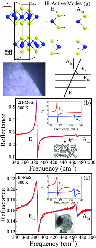
Figure 1: (Color online) (a) Crystal structure of 2H-MoS₂,Schonfeld1983 schematic view of the displacement patterns of the infrared-active modes, photo of a typical pressed pellet sample, and diagram for tilted oscillators. (b) Close-up view of the 300 K reflectance spectra of 2H-MoS₂ powder. The red solid curve is experimental data and the blue dashed line is a fit according to Eqs. (25) and (28). The insets show the dielectric constant and a schematic view of the 2H-MoS₂ platelets in a pressed pellet sample. (c) Close-up view of the 300 K reflectance of IF-MoS₂. An identical color scheme and line type is employed. The insets show the dielectric response and a high resolution TEM image of an IF-MoS₂ nanoparticle.

Table 1: Apparent parameters extracted from an oscillator fit to the measured reflectance spectrum of 2H-MoS₂ powder, and the intrinsic parameters from a single crystal sample. Wieting1971

	$\widetilde{S}_{j}$	$\widetilde{\epsilon}(\infty)$	$S_{j}$	$\epsilon(\infty)$
$E_{1u}$	0.114	10.3	0.20	15.2
$A_{2u}$	0.0036		0.030	6.2

Figure 1(b) displays a close-up view of the reflectance of 2H-MoS₂.Experiments As expected for a pressed powder sample, both the $E_{1u}$ and $A_{2u}$ modes are clearly observed. At normal incidence, the dielectric function is related to reflectance as:

$$R(\omega)={\displaystyle{\left|\frac{\sqrt{\epsilon(\omega)}-1}{\sqrt{\epsilon(\omega)}+1}\right|}}^{2}.$$ (25)

Equation (25) is formally valid for single-bounce reflectance at the interface of 2 semi-infinite media. For the case of real materials with finite thickness, sample thickness must be sufficient to assume that there is no back reflectance. Large attenuation due to a strong resonance is helpful here.

A fit to the 2H-MoS₂ powder data using Eqs. (23) and (25) (Fig. 1(b)) allows us to extract $\widetilde{\varepsilon}(\infty)=10.3$, $\widetilde{S}_{E_{1u}}=0.114$ and $\widetilde{S}_{A_{2u}}=0.0036$ (Table I). We refer to these values as “apparent oscillator parameters” because they are obtained from direct fits to the measured powder spectrum. They are distinct from the “intrinsic parameters” that are useful for evaluation of Born and ionic charge.

The apparent and intrinsic oscillator parameters are related according to Eqs. (24a- 24c) by the oscillator orientation. For MoS₂, one has:

$$\widetilde{\varepsilon}(\infty) = 1+[\varepsilon_{E_{1u}}(\infty)-1]\langle\cos^{2}(\theta_{E_{1u}})\rangle v$$ (26a)

$$+ [\varepsilon_{A_{2u}}(\infty)-1]\langle\cos^{2}(\theta_{A_{2u}})\rangle v$$

$$\widetilde{S}_{E_{1u}} = S_{E_{1u}}\langle\cos^{2}(\theta_{E_{1u}})\rangle v$$ (26b)

$$\widetilde{S}_{A_{2u}} = S_{A_{2u}}\langle\cos^{2}(\theta_{A_{2u}})\rangle v.$$ (26c)

Here, $$v=0.7$$ is the relative density of the unoriented pressed pellet compared with that of the single crystal.Experiments ; NoteDensity A benchmark is now needed to related the apparent and intrinsic oscillator parameters.

Fortunately, the polarized infrared reflectance of a 2H-MoS₂ single crystal has been studied by Wieting et al.Wieting1971 Fits to the reflectance yield $\epsilon(\infty)_{E_{1u}}=15.2$, $\epsilon(\infty)_{A_{2u}}=6.2$, $S_{E_{1u}}=0.20$, and $S_{A_{2u}}=0.03$ (Table 1). These intrinsic parameters are appropriate benchmarks for the our pellet samples, because they are made of $\mu m$ sized powders, for which the surface effect can be ignored as a good approximation.

In Eqs. (26a - 26c), the only unknowns are $\langle\cos^{2}(\theta_{E_{1u}})\rangle$ and $\langle\cos^{2}(\theta_{A_{2u}})\rangle$. Fig. 1(b) shows a schematic view of the pressed pellet of 2H- powder. Since the polarizations of the two modes are orthogonal, one has $\theta_{E_{1u}}+\theta_{A_{2u}}=\frac{\pi}{2}$. Hence, $\langle\cos^{2}(\theta_{E_{1u}})\rangle+\langle\cos^{2}(\theta_{A_{2u}})\rangle=1$, meaning that there is only one unknown, say, $\langle\cos^{2}(\theta_{E_{1u}})\rangle$. Using Eqs. (26b-26c), we find two independent values as 0.81 and 0.83 in good agreement with each other. To further check the self-consistency, we calculated $\widetilde{\epsilon}(\infty)$ using Eq. (26a) using an average value of $\langle\cos^{2}(\theta_{E_{1u}})\rangle$ = 0.82, yielding $\widetilde{\epsilon}(\infty)=9.8$, in excellent agreement with that obtained by direct fitting techniques ($\widetilde{\epsilon}(\infty)=10.3$). In addition to confirming the validity of our approach, this self-consistency also shows that the pressed powder sample of 2H-MoS₂ will have the same Born effective charge as the single crystal,Wieting1971 ; Sun2009 which, of course, it must. The dielectric response $\varepsilon_{1}$ was calculated using the intrinsic parameters of Ref. Sun2009, and is plotted in the inset of Fig. 1(b). The dispersive response is typical of an anisotropic insulator with two vibrational modes.

The availability of $\sim$30 - 70 nm average diameter nested MoS₂ nanoparticles provides an opportunity to investigate the impact of finite length scale effects on chemical bonding.Sun2009 Figure 1(c) displays a close-up view of the measured far infrared reflectance along with an oscillator fit. The apparent parameters obtained from this fit can be scaled toward a set of intrinsic oscillator parameters using the orientation and density corrections outlined above.Sun2009 From an analysis of these intrinsic oscillator strengths and high frequency dielectric constants along with mode frequencies, we can extract Born and local effective charges for the nanoparticles.Sun2009 In the intralayer direction, we find that the Born effective charge of the nanoparticles is 0.69 $e$ in the intralayer direction, significantly lower than that of the layered bulk (1.11 $e$). Here, $e$ is the charge of an electron. We attribute this difference to structural strain (and resulting change in intralayer polarizability) in the nanoparticles.Sun2009 The Born effective charge of the nanoparticles remains unchanged in the interlayer direction (0.52 $e$). The dielectric constant was again calculated using intrinsic parametersSun2009 and is plotted in the inset of Fig. 1(c). Clearly, the dispersive response of the nanoparticles is different from that of the bulk in the intralayer direction. They are the same in the interlayer direction.

Extension of Born and local (or ionic) charge concepts to nanomaterials is an important advance because most are not (and may never be) available in an oriented form.Long2007 ; Tenne2004 ; Poudel2008 ; Hochbaum2008 ; Boukai2008 ; Cao2007 Indeed, emerging mechanical and tribological applications of nanoscale MoS₂ require bulk quantities of powder with careful size-shape control but no orientational control. At the same time, the relationship between engineering properties such as solid state lubricationRapoport1997 ; Seifert2000 ; Remskar2007 and the microscopic aspects of charge and bonding is an open and interesting question that deserves further study.

VII Conclusion

We present an application of the Lorentz model in which fits to vibrational spectra or a Kramers Kronig analysis of the reflectance are employed along with several useful formalisms to quantify microscopic charge and polarizability in unoriented (powdered) materials. This paper provides a systematic development of the operative equations and a discussion of the conditions under which such techniques can be employed. We demonstrate the workability of our approach by analyzing the vibrational response of a layered transition metal dichalcogenide, and we include an evaluation of Born and local (or ionic charge) of its nanoscale analog to illustrate the modern utility. The extension to assess size effects advances the field of nanoscience and, at the same time, retains many attractive features of optical spectroscopy and the traditional Lorentz model.

Appendix A Other frameworks

For applications, it can be convenient to use other forms of Eq. (7) that are written in terms of parameters that are more related to the experimental observations. Before stepping into that, we take a careful look at Eq. (7) and note that there are only three independent parameters: $\alpha$, $q$, and $\omega_{0}$. Other three-variable sets offer equivalent expressions. Some of these are detailed below.

A.1 $\varepsilon(0)$, $\varepsilon(\infty)$ and $\omega_{TO}^{2}$ framework

This is a very useful framework because $\varepsilon(0)$, $\varepsilon(\infty)$, and $\omega_{TO}^{2}$ can all be straightforwardly extracted from the optical spectra.

A.1.1 Collinear Oscillators

Equation (8a) is already very close to employing this new set of parameters. Let’s define:

$$\varepsilon(0) = (1+\frac{\alpha/V}{1-\eta\alpha/V})+\frac{q^{2}}{\epsilon_{0}mV(1-\eta\alpha/V)^{2}}\frac{1}{\omega_{TO}^{2}}$$ (27)

$$= \varepsilon(\infty)+\frac{q^{2}}{\epsilon_{0}mV(1-\eta\alpha/V)^{2}}\frac{1}{\omega_{TO}^{2}}$$

Then,

$$A=\frac{q^{2}}{mV(1-\eta\alpha/V)^{2}}=\omega_{TO}^{2}[\varepsilon(0)-\varepsilon(\infty)]$$

with parameters $\varepsilon(0)$, $\varepsilon(\infty)$, and $\omega_{TO}^{2}$, one can rewrite Eq. (7):

$$\varepsilon=\varepsilon(\infty)+\omega_{TO}^{2}\frac{\varepsilon(0)-\varepsilon(\infty)}{\omega_{TO}^{2}-\omega^{2}-i\gamma\omega}$$ (28)

• $\omega_{0}^{2}$

It is a bit tedious, but not so difficult to show that:

$$\omega_{0}^{2}=\omega_{TO}^{2}\frac{\varepsilon(\infty)+1/\eta-1}{\varepsilon(0)+1/\eta-1}$$

• Ionic effective charge

$$q^{2} = \epsilon_{0}mV(1-\eta\alpha/V)^{2}A$$ (29)

$$= \epsilon_{0}mV(1-\eta\alpha/V)^{2}\omega_{TO}^{2}[\varepsilon(0)-\varepsilon(\infty)]$$

$$= \epsilon_{0}mV\frac{\omega_{TO}^{2}[\varepsilon(0)-\varepsilon(\infty)]}{\eta^{2}[\varepsilon(\infty)+1/\eta-1]^{2}}$$

• Born effective charge

$$q_{B}^{2}=\epsilon_{0}mV\omega_{TO}^{2}[\varepsilon(0)-\varepsilon(\infty)]$$ (30)

• $\omega_{LO}^{2}$

By definition, $\omega_{LO}$, $\varepsilon=0$ for a longitudinal mode. Using Eq. (28) (and ignoring $i\gamma\omega$), one has

$$0=\varepsilon(\infty)+\omega_{TO}^{2}\frac{\varepsilon(0)-\varepsilon(\infty)}{\omega_{TO}^{2}-\omega_{LO}^{2}}$$ (31)

which gives the Lyddane-Sachs-Teller relation,Ashcroft1976

$$\frac{\omega_{LO}^{2}}{\omega_{TO}^{2}}=\frac{\varepsilon(0)}{\varepsilon(\infty)}$$ (32)

One can write out $\omega_{LO}^{2}$ in terms of microscopic parameters $\alpha$, $q$ and $\omega_{0}$ using the Lyddane-Sachs-Teller relation as follows:

$$\omega_{LO}^{2} = \omega_{TO}^{2}\frac{\varepsilon(0)}{\varepsilon(\infty)}$$ (33)

$$= \omega_{TO}^{2}\frac{\varepsilon(\infty)+A\frac{1}{\omega_{TO}^{2}}}{\varepsilon(\infty)}$$

$$= \omega_{TO}^{2}+\frac{A}{\varepsilon(\infty)}$$

$$= \omega_{0}^{2}-\frac{q^{2}\eta}{\epsilon_{0}mV(1-\eta\alpha/V)}$$

$$+\frac{q^{2}}{\epsilon_{0}mV(1-\eta\alpha/V)^{2}}\frac{1}{1+\frac{\alpha/V}{1-\eta\alpha/V}}$$

$$= \omega_{0}^{2}+\frac{q^{2}}{\epsilon_{0}mV}\frac{1-\eta}{1+(1-\eta)\alpha/V}$$

Note that $\omega_{LO}^{2}$ is large than $\omega_{0}^{2}$, while $\omega_{TO}^{2}$ is smaller than $\omega_{0}^{2}$.

A.1.2 Multiple Collinear Oscillators

$$\varepsilon=1+\underset{j}{\sum}[\varepsilon_{j}(\infty)-1]+\underset{j}{\sum}\omega_{TO,j}^{2}\frac{\varepsilon_{j}(0)-\varepsilon_{j}(\infty)}{\omega_{TO,j}^{2}-\omega^{2}-i\gamma_{j}\omega}$$ (34)

A.1.3 Tilted Oscillators

$$\varepsilon = 1+[\varepsilon(\infty)-1)]\langle\cos^{2}(\theta)\rangle$$ (35)

$$+ \omega_{TO}^{2}\frac{\varepsilon(0)-\varepsilon(\infty)}{\omega_{TO}^{2}-\omega^{2}-i\gamma\omega}\langle\cos^{2}(\theta)\rangle$$

A.1.4 Multiple Tilted Oscillators

$$\varepsilon(\{\theta_{j}\}) = 1+\underset{j}{\sum}[\varepsilon_{j}(\infty)-1]\cos^{2}(\theta_{j})$$

$$+\underset{j}{\sum}\omega_{TO,j}^{2}\frac{\varepsilon_{j}(0)-\varepsilon_{j}(\infty)}{\omega_{TO,j}^{2}-\omega^{2}-i\gamma_{j}\omega}\cos^{2}(\theta_{j})$$

$$\widetilde{\varepsilon} =\langle\varepsilon(\{\theta_{j}\})\rangle$$

$$=1+\underset{j}{\sum}[\varepsilon_{j}(\infty)-1]\langle\cos^{2}(\theta_{j})\rangle$$

$$+\underset{j}{\sum}\omega_{TO,j}^{2}\frac{\varepsilon_{j}(0)-\varepsilon_{j}(\infty)}{\omega_{TO,j}^{2}-\omega^{2}-i\gamma_{j}\omega}\langle\cos^{2}(\theta_{j})\rangle$$ (36)

A.2 $\varepsilon(\infty)$, $\omega_{TO}^{2}$ and $\omega_{LO}^{2}$ framework

A.2.1 Collinear oscillators

Another choice is to use $\varepsilon(\infty)$, $\omega_{TO}^{2}$, and $\omega_{LO}^{2}$. Using the Lyddane-Sachs-Teller relation, Eq. (32), one can eliminate $\varepsilon(0)$, which yields

$$\varepsilon=\varepsilon(\infty)+\varepsilon(\infty)\frac{\omega_{LO}^{2}-\omega_{TO}^{2}}{\omega_{TO}^{2}-\omega^{2}-i\gamma\omega}$$ (37)

• Ionic effective charge

$$q^{2} = \epsilon_{0}mV(1-\eta\alpha/V)^{2}A$$ (38)

$$= \epsilon_{0}mV(1-\eta\alpha/V)^{2}\varepsilon(\infty)(\omega_{LO}^{2}-\omega_{TO}^{2})$$

$$= \epsilon_{0}mV\frac{\varepsilon(\infty)(\omega_{LO}^{2}-\omega_{TO}^{2})}{\eta^{2}[\varepsilon(\infty)+1/\eta-1]^{2}}$$

• Born effective charge

$$q_{B}^{2}=\epsilon_{0}mV\varepsilon(\infty)(\omega_{LO}^{2}-\omega_{TO}^{2})$$ (39)

A.2.2 Multiple Collinear Oscillators

$$\varepsilon=1+\underset{j}{\sum}[\varepsilon_{j}(\infty)-1]+\underset{j}{\sum}\varepsilon_{j}(\infty)\frac{\omega_{LO,j}^{2}-\omega_{TO,j}^{2}}{\omega_{TO,j}^{2}-\omega^{2}-i\gamma_{j}\omega}$$ (40)

A.2.3 Tilted Oscillators

$$\varepsilon = 1+[\varepsilon(\infty)-1]\langle\cos^{2}(\theta)\rangle$$ (41)

$$+ \varepsilon(\infty)\frac{\omega_{LO}^{2}-\omega_{TO,j}^{2}}{\omega_{TO}^{2}-\omega^{2}-i\gamma\omega}\langle\cos^{2}(\theta)\rangle$$

A.2.4 Multiple Tilted Oscillators

$$\varepsilon(\{\theta_{j}\}) =1+\underset{j}{\sum}[\varepsilon_{j}(\infty)-1]\cos^{2}(\theta_{j})$$

$$+\underset{j}{\sum}\varepsilon_{j}(\infty)\frac{\omega_{LO,j}^{2}-\omega_{TO,j}^{2}}{\omega_{TO,j}^{2}-\omega^{2}-i\gamma_{j}\omega}\cos^{2}(\theta_{j})$$ (42)

$$\widetilde{\varepsilon} =\langle\varepsilon(\{\theta_{j}\})\rangle$$

$$=1+\underset{j}{\sum}[\varepsilon_{j}(\infty)-1]\langle\cos^{2}(\theta_{j})\rangle$$

$$+\underset{j}{\sum}\varepsilon_{j}(\infty)\frac{(\omega_{LO,j}^{2}-\omega_{TO,j}^{2})}{\omega_{TO,j}^{2}-\omega^{2}-i\gamma_{j}\omega}\langle\cos^{2}(\theta_{j})\rangle$$ (43)

References

• (1) M. Born, Phys. Z. 19, 539 (1918).
• (2) B. Szigeti, Proc. R. Soc. London A 204, 51 (1950).
• (3) N. W. Ashcroft, and N. D. Mermin, Solid State Physics (Thomson Learning, New York, 1976).
• (4) C. Kittel, Introduction to Solid State Physics (Wiley, New York, 1966).
• (5) M. Born and K. Huang, Dynamic Theory of Crystal Lattices (Oxford University Press, London, 1954).
• (6) K. W. Lee and W. E. Pickett, Phys. Rev. B 68, 085308 (2003).
• (7) M. D. Fontana, G. Metrat, J. L. Servoin, and F. Gervais, J. Phys. C 17, 483 (1984).
• (8) W. Zhong, R.D. King-Smith, and D. Vanderbilt, Phys. Rev. Lett. 72, 3618 (1994).
• (9) J.W. Long and D.R. Rolison, Acc. Chem. Res. 40, 854 (2007).
• (10) R. Tenne and C. N. R. Rao, Phil. Trans. R. Soc. A 362, 2099 (2004).
• (11) B. Poudel, Q. Hao, Y. Ma, Y. C. Lan, A. Minnich, B. Yu, X. Yan, D. Z. Wang, A. Muto, D. Vashaee, X. Y. Chen, J. M. Liu, M. S. Dresselhaus, G. Chen, and Z. Ren, Science 320, 634 (2008).
• (12) A. I. Hochbaum, R. K. Chen, R. D. Delgado, W. J. Liang, E. C. Garnett, M. Najarian, A. Majumdar, and P. D. Yang, Nature 451, 163 (2008).
• (13) A. I. Boukai, Y. Bunimovich, J. Tahir-Kheli, J. K. Yu, W. A. Goddard, and J. R. Heath, Nature 451, 168 (2008).
• (14) J. Cao, J.L. Musfeldt, S. Mazumdar, N.A. Chernova, and M.S. Whittingham, Nano. Lett. 7, 2351 (2007).
• (15) G.L. Carr, S. Perkowitz, and D.B. Tanner, Infrared and Millimeter Waves 13, 177 (1985).
• (16) Q.-C. Sun, X. S. Xu, L. I. Vergara, R. Rosentsveig, and J. L. Musfeldt, Phys. Rev. B 79, 205405 (2009).
• (17) T. J. Wieting and J. L. Verble, Phys. Rev. B 3, 4286 (1971).
• (18) S. I. Uchida and S. Tanaka, J. Phys. Soc. Jpn 45, 153 (1978).
• (19) F. Wooten, Optical Properties of Solids (New York, Academic Press, 1972).
• (20) K. Huang and R. Q. Han, Solid State Physics (in Chinese) (Higher Education Press, China, 1988).
• (21) X. Gonze and C. Lee, Phys. Rev. B 55, 10355 (1997).
• (22) B. Schonfeld, J. J. Huang and S. C. Moss, Acta Crystallogr. Sect. B 39, 404 (1983).
• (23) J. L. Verble and T. J. Wieting, Phys. Rev. Lett. 25, 362 (1970).
• (24) IF-MoS2 was prepared as described previously.Sun2009 2H-MoS2 was purchased directly from Alfa Aesar (99%). Pressed pellet samples were prepared using low pressure (see Fig. 1(a)). The theoretical density of 2H-MoS2 single crystal is 4.996 g/cm3, and the actual densities of 2H- and IF- pellets are $\sim$3.5 g/cm3. Pellet densities are therefore $\sim$70% of the single crystal density, a difference that we correct for in our analysis. We checked that there is no significant infrared transmittance of the samples (thickness between 1.0 and 1.3 mm), indicating large attenuation due to strong resonance. Near normal infrared reflectance was measured using a Bruker 113V Fourier transform infrared spectrometer. A helium-cooled bolometer detector was employed in the far-infrared for added sensitivity. Both 0.5 and 2 cm-1 resolution were used in the infrared.Sun2009
• (25) For far infrared spectroscopy, the wavelength of the light is usually much larger than the particle size. Therefore, the measured oscillator strength is proportional to the concentration of the oscillators, which is inversely proportional to the mass density of the powder sample.
• (26) L. Rapoport, Y. Bilik, Y. Feldman, M. Homyonfer, S. R. Cohen, and R. Tenne, Nature 387, 791 (1997).
• (27) G. Seifert, H. Terrones, M. Terrones, G. Jungnickel, and T. Frauenheim, Phys. Rev. Lett. 85, 146 (2000).
• (28) M. Remskar, A. Mrzel, M. Virsek, and A. Jesih, Adv. Mater. 19, 4276 (2007).