Radio properties of the low surface brightness SNR G65.2+5.7

Abstract

Context. SNR G65.2+5.7 is one of few supernova remnants (SNRs) that have been optically detected. It is exceptionally bright in X-rays and the optical [O III]-line. Its low surface brightness and large diameter ensure that radio observations of SNR G65.2+5.7 are technically difficult and thus have hardly been completed.

Aims. Many physical properties of this SNR, such as spectrum and polarization, can only be investigated by radio observations.

Methods. The $\lambda$11 cm and $\lambda$6 cm continuum and polarization observations of SNR G65.2+5.7 were completed with the Effelsberg 100-m and the Urumqi 25-m telescopes, respectively, to investigate the integrated spectrum, the spectral index distribution, and the magnetic field properties. Archival $\lambda$21 cm data of the Effelsberg 100-m telescope were also used.

Results. The integrated flux densities of G65.2+5.7 at $\lambda 11$ cm and $\lambda 6$ cm are $21.9\pm 3.1$ Jy and 16.8$\pm$1.8 Jy, respectively. The power-law spectrum ($S\sim\nu^{\alpha}$) is well fitted by $\alpha=-0.58\pm 0.07$ from 83 MHz to 4.8 GHz. Spatial spectral variations are small. Along the northern shell, strong depolarizion is observed at both wavelengths. The southern filamentary shell of SNR G65.2+5.7 is polarized by as much as 54% at $\lambda 6$ cm. There is significant depolarization at $\lambda 11$ cm and confusion with diffuse polarized Galactic emission. Using equipartition principle, we estimated the magnetic field strength for the southern filamentary shell to be between 20 $\mu$G (filling factor 1) and 50 $\mu$G (filling factor 0.1). A faint HI shell may be associated with the SNR.

Conclusions. Despite its unusually strong X-ray and optical emission and its very low surface brightness, the radio properties of SNR G65.2+5.7 are found to be typical of evolved shell-type SNRs. SNR G65.2+5.7 may be expanding in a pre-blown cavity as indicated by a deficit of HI gas and a possible HI-shell.

1 Introduction

SNRs of low radio surface brightness and large diameter are difficult to identify in radio continuum surveys. The weakest source detected in our Galaxy is SNR G156.2+5.7 (Reich et al. 1992), which has a surface brightness $\rm\Sigma_{1GHz}\sim 5.8\times 10^{-23}Wm^{-2}Hz^{-1}sr^{-1}$, and SNR G65.2+5.7 is a similar weak object, whose low surface brightness may be caused by a low ambient magnetic field strength or a low electron density. In most cases, the supernova has exploded in a low-density medium, for instance in an interarm region or in a pre-existing cavity. In the case of a pre-existing cavity substantial radio emission is visible for only a relatively short time interval as the shock collides with the dense shell.

Gull et al. (1977) first identified G65.2+5.7 as a large diameter SNR located in the Cygnus region in an optical emission line survey, where it appeared to be exceptionally bright in [O III]. This is indicative of high shock velocities typically for an expanding SNR shell. Reich et al. (1979) used the Effelsberg 100-m telescope at $\lambda 21$cm to map G65.2+5.7 and confirmed its identification as a SNR by its non-thermal emission.

G65.2+5.7 is a bright soft X-ray source for which Shelton et al. (2004) analysed ROSAT PSPC data, classifying the SNR as a “thermal composite” object with a cool, dense shell and no X-ray emission. Bright centrally peaked thermal X-ray emission dominates the interior of these SNRs, although they are rare. W44 is another example (Cox et al. 1999), which is younger than G65.2+5.7.

Distance estimates were made by various authors. Boumis et al. (2004) used proper motion and expansion measurements of the remnant’s optical filament edges and obtained 770$\pm$200 pc. In the following, we assume a distance of 800 pc. The apparent size of G65.2+5.7 is about $4\degr\times 3\aas@@fstack{\circ}3$ (Gull et al. 1977), corresponding to a physical size of 56 pc $\times$ 46 pc. The centre of the SNR is located about 80 pc above the Galactic plane. G65.2+5.7 appears to be an evolved object, although its age is uncertain: It may be as old as $3\times 10^{5}$ years if one assumes an average shock velocity of $\sim$ 50 km s^-1 (Gull et al. 1977; Reich et al. 1979). Optical observations show the velocities in the range between 90 km s^-1 and 140 km s^-1 (Mavromatakis et al. 2002). ROSAT X-ray data infer shock velocities of about 400 km s^-1 (Schaudel et al. 2002), which implies an age of $2.8\times 10^{4}$ years.

The Princeton-Arecibo pulsar survey found a pulsar, PSR J1931+30, in the direction of G65.2+5.7 (Camilo et al. 1996). From its dispersion measure of 56$\pm 11$ cm^-3pc, a distance of about 3 kpc is inferred, which excludes a physical association with G65.2+5.7.

The only radio observations of G65.2+5.7 have been those by Reich et al. (1979) at $\lambda 21$ cm and the low-resolution, low-frequency observations by Kovalenko et al. (1994), reflecting the difficulty in mapping these faint large-diameter objects. With the availability of new sensitive and highly stable receivers, it is now possible to map this object also at higher frequencies with arc minute angular resolution and investigate its spectral properties and magnetic field structure. We describe new sensitive radio measurements in total power and linear polarization at $\lambda$11 cm and $\lambda$6 cm of G65.2+5.7 and present results on the spectral and polarization analysis in Sect. 2. A brief discussion of the radio results with respect to observations at other wavelengths is given in Sect. 3, followed by a summary in Sect. 4.

2 Observations and result analyses

Continuum and linear polarization observations of G65.2+5.7 at $\lambda$6 cm (4800 MHz) were completed with the 25-m telescope at Nanshan station of the Urumqi Observatory. The $\lambda$6 cm receiver is a copy of a receiver used at the Effelsberg 100-m telescope and was installed in 2004 for the $\lambda$6 cm polarization survey of the Galactic plane (Sun et al. 2007). Sun et al. (2006) described the performance of the receiving system in some detail. Between 2006 and 2007, nine observations of G65.2+5.7 were completed, which were centered at $\rm\alpha_{2000}=19^{h}33^{m}6^{s}$, $\delta_{2000}=31\degr 17\arcmin 31\arcsec$. The map size, $\Delta$RA $\times$ $\Delta$Dec, was $5\degr\times 4\aas@@fstack{\circ}5$. The maps were scanned either along the RA- or Dec-direction with a telescope scan velocity of $4\arcmin$/sec.

Table 1: Observational parameters

Wavelength	$\lambda$6 cm	$\lambda$11 cm
Frequency	4800 MHz	2639 MHz
Bandwidth	600 MHz	80 MHz
HPBW [′]	9.5	4.4
apperture efficiency[%]	62	53
beam efficiency[%]	67	58
Tsys[K]	22	17
T${}_{B}[K]$/S[Jy]	0.164	2.52
Main Calibrator	3C286	3C286
Flux Density	7.5 Jy	11.5 Jy
Polarization Percentage	11.3%	9.9%
Polarization Angle	33$\degr$	33$\degr$
No. of coverages	9	7
pixel integration time [sec]	7	3.5
r.m.s in TP [mK]	0.7	3.5
r.m.s in PI [mK]	0.3	1.7

The observations of G65.2+5.7 at $\lambda$11 cm (2639 MHz) were completed with a receiver installed at the secondary focus of the Effelsberg 100-m telescope in 2005. They were carried out in the same way as the observations with the Urumqi telescope. G65.2+5.7 was observed seven times in autumn 2007 mostly in clear sky. In Table 1, we list the parameters of the $\lambda$6 cm and $\lambda$11 cm observations with the data of the main calibrator 3C286. The $\lambda$11 cm observations were carried out with a 8-channel narrow band polarimeter. Each channel has a bandwidth of 10 MHz. The centre frequencies are separated by 10 MHz and range from 2604 MHz to 2674 MHz. The 9th broadband-channel has a bandwidth of 80 MHz and is centered on 2639 MHz. This channel was used for all observations in which no narrow band interference was present, which was the case for the observations of G65.2+5.7.

The data processing was completed in exactly the same way as described by Xiao et al. (2008) for the observations of the SNR S147, an object of similar size and faintness as G65.2+5.7. In brief, the individual maps for Stokes I, U, and Q were checked and low quality data caused by interference were removed. The baselines for Stokes I were corrected by subtracting a second order polynomial fit to the lower emission envelope; this step removed ground emission variations and also the smooth increase in Galactic emission towards the Galactic plane evident in the long scans. We suppressed scanning effects for U/Q maps by applying the “unsharp masking” method described by Sofue & Reich (1979). Finally, all maps were combined using the PLAIT-algorithm (Emerson & Gräve 1988).

2.1 Total intensity and linear polarization maps

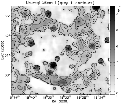
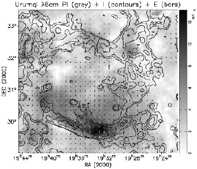
Figure 1: The Urumqi $\lambda$6 cm map of G65.2+5.7 with an angular resolution of $9\aas@@fstack{\prime}5$. The upper panel shows the distribution of total intensities. The lower panel shows polarized intensities (PI) in grey superimposed on total intensity contours (with point-like sources subtracted) and bars for E-field direction. The length of the bars is proportional to PI. Polarized intensity of 1 mK T_B corresponds to a bar-length of $0\aas@@fstack{\prime}86$. Both panels show total intensity contours starting at 0 mK T_B and increasing $\rm 2^{n}\times 3\sigma_{I}$, where n=0,1,2,3$\cdots$ and $\rm\sigma_{I}=0.7$ mK T_B.

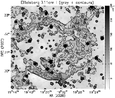
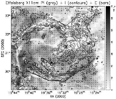
Figure 2: Same as Fig. 1, but for the Effelsberg $\lambda$11 cm map with an angular resolution of $4\aas@@fstack{\prime}4$. Polarized intensity of 1 mK T_B corresponds to a bar-length of $0\aas@@fstack{\prime}25$. Total intensity contours start at 21 mK T_B and increase in steps of $\rm 2^{n}\times 3\sigma_{I}$ with n=0,1,2,3$\cdots$, where $\rm\sigma_{I}=3.5$ mk T_B.

The Urumqi $\lambda$6 cm total intensity map of G65.2+5.7 and the corresponding polarization intensity map superimposed with vectors in the E-field direction are shown in Fig. 1. From low-intensity areas in the maps, we measured an r.m.s.-noise in total intensity and in linear polarized intensity of 0.7 mK T_B and 0.3 mK T_B, respectively. The $\lambda$11 cm maps are shown in Fig. 2. The r.m.s.-noise was measured to be 3.5 mK T_B in total intensity and 1.7 mK T_B in linear polarized intensity. Because of the higher angular resolution of the $\lambda$11 cm map of $4\aas@@fstack{\prime}4$, the filamentary elliptical shell is more clearly detected.

For the spectral index analysis we also used an archival $\lambda$21 cm map obtained with the Effelsberg 100-m telescope in November 1987 at 1408 MHz with a bandwidth of 20 MHz and an angular resolution of $9\aas@@fstack{\prime}4$. These observations were made in due course with a $\lambda$21 cm Galactic plane survey in total intensity (Reich et al. 1990), which covers the plane within an interval of $\pm 4\degr$ in latitude, so that a small part of G65.2+5.7 is included there. Polarization data were taken from a section of the “$\lambda$21 cm Effelsberg Medium Latitude Survey” (Reich et al. 2004), which was combined with data from the DRAO 1.4 GHz polarization survey (Wolleben et al. 2006) to help ensure detection of any missing large-scale polarized emission. The $\lambda$21 cm map is shown in Fig. 3.

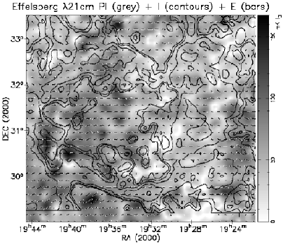
Figure 3: Effelsberg $\lambda$21 cm polarized intensity map of G65.2+5.7 with an angular resolution of $9\aas@@fstack{\prime}4$. The length of the bars is proportional to PI. Polarized intensity of 1 mK T_B corresponds to a bar-length of $0\aas@@fstack{\prime}075$. Contours show total intensities with compact sources removed starting at 66 mK T_B and increasing in steps of $\rm 2^{n}\times 36\leavevmode\nobreak\ mK\leavevmode\nobreak\ T_{\rm B}$ with n=0,1,2,3$\cdots$.

2.2 The integrated radio spectrum

To estimate the integrated flux density of the remnant, we subtracted 20 bright point-like sources by Gaussian fitting within the area of the SNR, and a few just outside, from the $\lambda$11 cm map and 16 sources from the $\lambda$6 cm map. The sources are listed in Table 2. The position accuracy of the two maps is about $7\arcsec$ on average, which was estimated by comparing the source positions with those from the NVSS (Condon et al. 1998).

Table 2: Bright sources in the area of SNR G65.2+5.7 fitted from the Effelsberg $\lambda$11 cm and Urumqi at $\lambda$6 cm maps, including source positions, flux densities from the NVSS at $\lambda$21 cm, as well as spectral indices. Sources ’outside’ G65.2+5.7 are listed for completeness.

	NVSS	NVSS	$S_{NVSS}$				$S_{11cm}$			$S_{6cm}$			$\alpha$	comment
	$\alpha_{2000}$	$\delta_{2000}$	(mJy)				(mJy)			(mJy)
1	19 23 25.26	30 42 35.4	574.	4$\pm$	19.	1	300	$\pm$	14	159	$\pm$	16	-0.83$\pm$0.05
2	19 25 13.64	30 31 18.9	70.	3$\pm$	2.	1	43	$\pm$	7	31	$\pm$	5	-0.81$\pm$0.19
3	19 25 27.29	31 29 23.9	384.	3$\pm$	12.	6	222	$\pm$	12	171	$\pm$	9	-0.64$\pm$0.07
4	19 26 16.04	32 35 51.6	105.	4$\pm$	3.	9	47	$\pm$	14				-1.28$\pm$0.49
5	19 26 40.65	32 56 55.9	67.	1$\pm$	3.	0	48	$\pm$	12				-0.53$\pm$0.42	3 unresolved sources
6	19 26 56.04	29 37 19.6	193.	2$\pm$	6.	0	111	$\pm$	6	67	$\pm$	17	-0.84$\pm$0.14	outside
7	19 27 11.53	29 52 54.5	51.	6$\pm$	2.	2	28	$\pm$	9	24	$\pm$	5	-0.77$\pm$0.21	outside
8	19 27 33.05	32 14 01.3	79.	2$\pm$	2.	8	52	$\pm$	9	43	$\pm$	8	-0.72$\pm$0.18
9	19 30 28.65	30 27 42.0	113.	1$\pm$	3.	4	71	$\pm$	4	37	$\pm$	4	-1.03$\pm$0.15
10	19 30 46.84	31 05 59.1	126.	2$\pm$	4.	4	62	$\pm$	8	43	$\pm$	9	-0.80$\pm$0.15
11	19 31 08.60	31 22 33.5	428.	6$\pm$	12.	9	311	$\pm$	11	232	$\pm$	14	-0.63$\pm$0.05	11/6cm fit
12	19 31 14.43	29 12 35.2	67.	7$\pm$	2.	1	59	$\pm$	16	55	$\pm$	5	-0.66$\pm$0.19	outside
13	19 32 45.08	31 06 10.7	35.	8$\pm$	1.	1	38	$\pm$	8				0.09$\pm$0.35
14	19 33 48.95	30 51 45.1	64.	7$\pm$	2.	0	90	$\pm$	15	98	$\pm$	8	0.14$\pm$0.07	11/6cm fit
15	19 34 19.84	29 20 07.4	65.	5$\pm$	2.	3	59	$\pm$	9	37	$\pm$	8	-0.84$\pm$0.20	outside
16	19 34 38.47	32 24 47.8	625.	7$\pm$	18.	8	299	$\pm$	13	146	$\pm$	13	-0.80$\pm$0.04
17	19 34 45.20	30 30 58.8	235.	2$\pm$	7.	1	469	$\pm$	14	579	$\pm$	23	0.35$\pm$0.11
18	19 35 34.24	30 08 00.9	688.	7$\pm$	23.	8	359	$\pm$	43	183	$\pm$	22	-0.81$\pm$0.04
19	19 35 56.39	33 08 22.0	77.	0$\pm$	2.	3	216	$\pm$	10	250	$\pm$	16	0.24$\pm$0.18	outside, 11/6cm fit
20	19 36 58.60	31 17 25.8	149.	7$\pm$	4.	5	93	$\pm$	9	55	$\pm$	14	-0.89$\pm$0.16
21	19 38 38.31	30 23 55.4	92.	6$\pm$	2.	8	172	$\pm$	15	171	$\pm$	18	-0.01$\pm$0.29	11/6cm fit
22	19 40 03.36	31 37 40.6	538.	5$\pm$	18.	4	353	$\pm$	15	220	$\pm$	17	-0.77$\pm$0.05
23	19 40 26.13	31 06 23.9	199.	4$\pm$	6.	0	112	$\pm$	15	61	$\pm$	8	-0.94$\pm$0.14
24	19 40 39.90	29 44 46.8	300.	1$\pm$	10.	6	147	$\pm$	9	73	$\pm$	17	-0.92$\pm$0.11	outside
25	19 42 14.83	32 15 38.7	177.	2$\pm$	5.	3	98	$\pm$	12				-0.93$\pm$0.23
26	19 42 29.66	32 24 46.9	83.	3$\pm$	2.	5	58	$\pm$	12				-0.58$\pm$0.35	outside
27	19 43 00.76	31 58 14.2	76.	3$\pm$	2.	3	60	$\pm$	10	43	$\pm$	16	-0.79$\pm$0.20
28	19 44 05.01	30 46 45.8	156.	6$\pm$	4.	7	82	$\pm$	4	37	$\pm$	12	-0.96$\pm$0.16	outside

We used the method of temperature-versus-temperature (TT) plot (Turtle et al. 1962) to adjust the base-levels of the entire SNR area at two wavelengths. Both maps were convolved to a common angular resolution of $10\arcmin$. In agreement with the TT-plot results for three different shell regions (see Sect. 3.3), we found a constant offset of $\rm-6\leavevmode\nobreak\ mK\leavevmode\nobreak\ T_{\rm B}$ at $\lambda$6 cm. At $\lambda$11 cm, we subtracted a “twisted” surface, which was defined by specific correction values at the four corners (3, 3, $-6$, and 3 mK T_B from lower left, right to upper left, right) of the map. The integrated flux densities were obtained by integrating the emission enclosed within polygons just outside the periphery of the SNR. From variations outside the SNR, we estimated a remaining uncertainty in the base-level setting of $\rm 1\leavevmode\nobreak\ mK\leavevmode\nobreak\ T_{\mathrm{B}}$ at $\lambda$6 cm and $\rm 2\ mK\ T_{\mathrm{B}}$ at $\lambda$11 cm. By assuming an estimated 5% calibration uncertainty, we obtained integrated flux densities of 16.8$\pm$1.8 Jy at $\lambda$6 cm and 21.9$\pm$3.1 Jy at $\lambda$11 cm.

In Fig. 4, these data are plotted together with flux density values from Reich et al. (1979) (408 MHz and 1415 MHz) and Kovalenko et al. (1994) (83 MHz and 111 MHz). All data are summarized in Table 3. For the Effelsberg $\lambda$21 cm map observed in 1987, we obtained the same flux density of $\rm 42.4\pm 4.1\$Jy for G65.2+5.7 that was obtained for the map published by Reich et al. (1979). We subtracted the flux densities of point-like sources listed in Table 2 by assuming a spectral index of $\alpha=-0.79$, which we decided on after caöculating the average by weighting the source spectral indices according to their flux densities. The linear fit to the integrated flux densities of G65.2+5.7 as shown in Fig. 4 yields a spectral index of $\alpha=-0.58\pm 0.07$.

Table 3: Integrated flux densities of G65.2+5.7, before ($S_{\nu}$) and after ($S_{\nu}cor$) subtraction of point-like sources within the boundary of SNR.

$\nu$	Resolution	$S_{\nu}$			$S_{\nu}$cor			Ref.
(MHz)	(arcmin)	(Jy)			(Jy)
83	310$\times$240	200.	0$\pm$	50	149.	2$\pm$	50	Kovalenko et al. (1994)
111	310$\times$240	175.	0$\pm$	40	134.	7$\pm$	40	Kovalenko et al. (1994)
408	37	91.	0$\pm$	15	76.	6$\pm$	15	Reich et al. (1979)
1415	9	42.	4$\pm$	4.6	37.	0$\pm$	4.6	Reich et al. (1979)
2639	4.4	.			21.	9$\pm$	3.1	this paper
4800	9.5	.			16.	8$\pm$	1.8	this paper

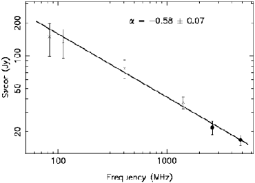
Figure 4: Spectrum of the integrated radio flux densities of G65.2+5.7. The spectral index is $\alpha=-0.58\pm 0.07$. All flux densities were corrected for the contribution of compact sources (Table 3).

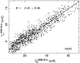
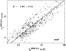
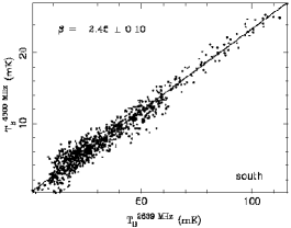
Figure 5: T-T plots for different shell sections of G65.2+5.7 between $\lambda$11 cm and $\lambda$6 cm.

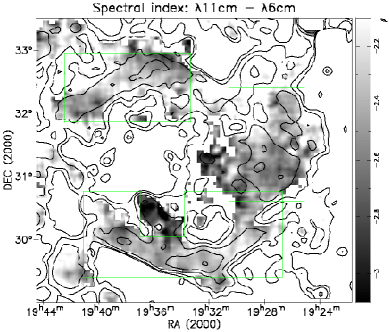
Figure 6: Spectral index map calculated between $\lambda$11 cm and $\lambda$6 cm at 10$\arcmin$ angular resolution for total intensities exceeding 12 mk T_B and 4 mk T_B at $\lambda$11 cm and $\lambda$6 cm, respectively. The overlaid contours show total intensities at $\lambda$11 cm starting at 12 mK T_B, increasing in steps of $\rm 2^{n}\times 3\sigma_{I}$, where n=0,1,2,3$\cdots$, and $\rm\sigma_{I}=2.2\leavevmode\nobreak\ mk\leavevmode\nobreak\ T_{\rm B}$. The regions used for TT-plots in Fig. 5 are indicated by boxes.

2.3 TT-plot spectral analysis

The TT-plot method used for relative zero-level setting in Sect. 2.2 was also used to investigate the spectrum of distinct emission structures in a way independent of a consistent base-level setting of both maps. Spectral index variations of structures within a source could then be recognized or the integrated spectrum checked. We smoothed both maps to $10\arcmin$ and applied this method for three different sections of the G65.2+5.7 shell, which are marked in Fig. 6. The results are shown in Fig. 5 for the $\lambda$11 cm/$\lambda$6 cm data. A clear temperature-temperature relation is evident in all cases. The same TT-plot procedure was used for the $\lambda$21 cm/$\lambda$6 cm data. The temperature spectral index $\beta(=\alpha-2)$ found from fitting the slope is $\beta_{11/6}=-2.45\pm 0.10$ and $\beta_{21/6}=-2.61\pm 0.24$ for the southern shell, $\beta_{11/6}=-2.46\pm 0.24$ and $\beta_{21/6}=-2.65\pm 0.27$ for the northeastern shell, and $\beta_{11/6}=-2.54\pm 0.44$ and $\beta_{21/6}=-2.71\pm 0.45$ for the western shell. The error in $\beta$ for the diffuse western part of the shell region is large, probably due to its weak emission and confusion with weak unresolved background sources, which could not be subtracted. All values agree with both each other and the spectral index of the integrated spectrum to within the errors. However, we always obtain somewhat steeper spectra for the $\lambda$21 cm/$\lambda$6 cm data than the $\lambda$11 cm/$\lambda$6 cm data, which reflects the slightly lower integrated flux density at $\lambda$11 cm relative to the fit shown in Fig. 4 and the marginally higher value we obtained at $\lambda$21 cm.

2.4 Spectral index map

The Urumqi $\lambda$6 cm and the Effelsberg $\lambda$11 cm maps with point-like sources removed and base-level corrected were both convolved to a common angular resolution of $10\arcmin$. We calculated the spectral index for each pixel from the brightness temperatures at the two frequencies. We defined a lower intensity limit of 4 mK T_B and 12 mK  T_B for the $\lambda$6 cm and $\lambda$11 cm map, respectively, to achieve reasonable spectral indices without the influence of noise and local distortions. We display the spectral index map between $\lambda$6 cm and $\lambda$11 cm in Fig. 6. Possible remaining variations in the base-levels at $\lambda$11 cm or $\lambda$6 cm cause a systematic uncertainty in the spectral indices of $\Delta\beta\sim 0.2$. The uncertainty is larger when total intensities are lower.

The filament emerging from the southern shell towards the north has a somewhat steeper spectrum than that of the southern shell. This is confirmed by $\beta_{11/6}=-2.75\pm 0.28$ obtained from TT-plot, although this spectral index value is within the errors of those obtained for the other shell regions.

Reich et al. (1979) found an indication of spectral flattening towards the centre of G65.2+5.7 of about $\Delta\beta\sim 0.3$ when comparing their Effelsberg $\lambda$21 cm map with low-resolution data at 408 MHz (Haslam et al. 1974). This finding cannot be verified by the present data. The emission in the central area is too faint at higher frequencies to derive meaningful spectral indices in relation to the base-level uncertainties.

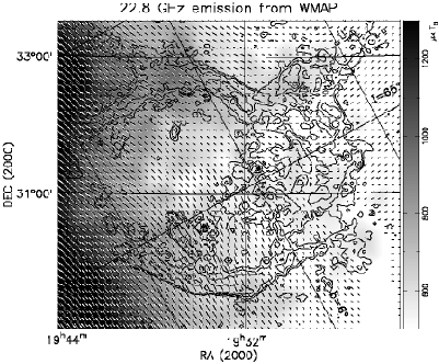
Figure 7: The WMAP 22.8 GHz map. The total intensity emission (grey-scale) map is smoothed to an angular resolution of $2\degr$ with polarization B-vectors overlaid. Their length is proportional to the polarized intensity. The overlaid contours show total intensities at $\lambda$11 cm at the same level as in Fig. 2 with compact sources removed.

2.5 The linear polarization properties of G65.2+5.7

The $\lambda$6 cm and $\lambda$11 cm polarization maps shown in the lower panels of Figs. 1 and 2 indicate the similar polarization features at the two frequencies. Four polarized patches appear at $\lambda$6 cm, three smaller and fainter ones located in the northern area of G65.2+5.7, and a single large patch covering the southern shell and part of the inner area of the SNR. Apart from the enhanced polarization along the SNR southern shell, most of the polarization structures might originate from polarized diffuse interstellar emission possibly mixed with polarized emission from the SNR of about similar strength. We note low polarized emission along the northern shell at both wavelengths.

As shown in Fig. 3 the $\lambda$21 cm polarization data do not indicate any polarized emission at all compared to G65.2+5.7, since neither the polarized intensity nor the polarization vectors change significantly in the direction of the SNR relative to its surroundings. This indicates that most of the polarized emission seen in this area at $\lambda$21 cm originates from the foreground within the distance to G65.2+5.7 of about 800 pc.

The large-scale emission components are missing in the two polarization maps at $\lambda$6 cm and $\lambda$11 cm, because the end-points of each scan in the individual U and Q maps were set to zero during data processing. This limits the interpretation of polarization structures (Reich 2006), except for the strong polarized region along the southern shell at $\lambda$6 cm.

Following Sun et al. (2007), we used the WMAP polarization data at 22.8 GHz (Page et al. 2007) to recover missing large-scale structures at $\lambda$6 cm. There is no signature of G65.2+5.7 in the Stokes U and Q maps at 22.8 GHz. The convolved 22.8 GHz PI map shows a smooth intensity increase below Galactic latitudes of about $5\aas@@fstack{\circ}5$. Above $5\aas@@fstack{\circ}5$, the orientation of the polarization B-vectors is less regular (Fig. 7). We convolved the WMAP 22.8 GHz U and Q maps corresponding to an angular resolution of $2\degr$ and scaled them to 4.8 GHz ($\lambda$6 cm) assuming a temperature spectral index of $\beta=-2.65$, which was taken from the spectral index map of total intensities between 408 MHz and 1420 MHz by Reich & Reich (1988). We assume the same spectral index for the Galactic diffuse polarized emission. The difference between the scaled WMAP data and the $\lambda$6 cm maps, when convolved to the same beam size of $2\degr$, results in an offset of $\rm-0.4\leavevmode\nobreak\ mK\leavevmode\nobreak\ T_{\rm B}$ for Stokes U and $\rm-2.3\leavevmode\nobreak\ mK\leavevmode\nobreak\ T_{\rm B}$ for Stokes Q, which is equivalent to $\rm 2.3\leavevmode\nobreak\ mK\leavevmode\nobreak\ T_{\rm B}$ of polarized intensity. The offsets were added to the original $\lambda$6 cm U and Q data. The polarized intensity map at $\lambda$6 cm derived from the restored data is shown in Fig. 8.

We then compared the $\lambda$6 cm polarization maps with and without absolute zero-level restoration. We found in general that the addition of missing large-scale polarization did not change the morphology of the observed polarization at $\lambda$6 cm significantly. The polarized signal from the southern shell of G65.2+5.7 was strong enough to remain almost unchanged when adding the large-scale emission component. Strong polarization emission of the diffuse interstellar medium near to the Galactic plane in the south-eastern area of the map is unrelated to G65.2+5.7. However, we note some changes in areas of lower polarized emission. For instance, the polarized emisssion is more pronounced in the direction of the extended HII-region LBN 150, also known as Sh2-96, ($\rm 19^{h}28.7^{m},+32\degr 41\arcmin$, J2000) in Fig. 8, which itself does not emit polarized emission, but may act as a Faraday screen by rotating polarized emission from larger distances.

The procedure for recovering missing large-scale emission by using the WMAP polarization data, needs to be modified in case the Faraday rotation is too large or becomes significant at longer wavelengths because of the $\lambda^{2}$-dependence of the polarization angle for a given RM. Therefore, it seems questionable that the $\lambda$11 cm U and Q maps should by corrected in the same way as the $\lambda$6 cm polarization data. The level of Galactic PI at $\lambda$11 cm, however, is calculated to be about $\rm 11.5\leavevmode\nobreak\ mK\leavevmode\nobreak\ T_{\rm B}$. This large-scale polarized signal needs to be compared with the observed polarized signals at $\lambda$11 cm, which are only three times stronger on the inner side of the southern shell and only twice as strong for the average polarization of the entire SNR. We conclude that the missing large-scale polarization is a serious contamination of the $\lambda$11 cm data and any RMs calculated from the $\lambda$11 cm and the $\lambda$6 cm data will by affected by an unknown amount by that effect.

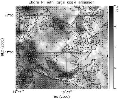
Figure 8: The $\lambda$6 cm polarized intensity map (grey scale) with large-scale polarized emission restored from WMAP 22.8 GHz polarization data. B-field vectors are shown for the case of negligible Faraday rotation. Contours show $\lambda$6 cm intensities as in Fig. 1.

2.6 The northern area of G65.2+5.7

The polarized emission seen in the northern area of the SNR is much weaker than in the southern area and not very clearly related to the SNR shell. Along the northern shell, depolarization at both $\lambda$11 cm and $\lambda$6 cm is evident, which may have various causes. Firstly, background polarization is depolarized by small-scale magneto-ionic fluctuations in the shell; secondly, polarized emission from the SNR shell has a different orientation and cancels, at least partly, the background emission; or, thirdly, Faraday rotation in the shell rotates background polarization in such a way that it cancels the foreground polarization. A combination of the different scenarios is certainly possible. We note that Mavromatakis et al. (2002) measured the highest thermal electron densities for the optical filaments in the northern shell, which may explain the high depolarization. The low percentage polarization in the northern area, compared to that of the southern shell, may indicate a less regular magnetic field. We conclude that the magnetic field properties along the northern shell cannot be determined reliably from the data available to us.

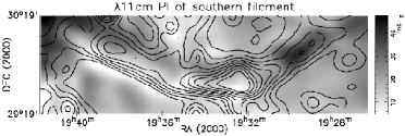
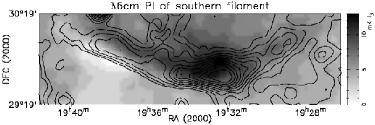
Figure 9: The observed polarized intensities in grey scales for the southern shell at $\lambda$11 cm and $\lambda$6 cm overlaid with contours of corresponding total intensities. Both maps are smoothed to $10\arcmin$ angular resolution.

2.7 The southern shell of G65.2+5.7

As shown in Fig. 9 the polarized emission at $\lambda$6 cm reaches its maximum at the southern shell. The polarization percentage of the southern shell locally is as high as 54% at $\lambda$6 cm. Lower polarized emission at $\lambda$11 cm at the same position indicates strong depolarization at this wavelength. Inside the shell the polarization percentage at $\lambda$11 cm is about 38%.

As expected for an evolved SNR, a well ordered magnetic field is detected in the shell. Rotating the polarization E-vectors shown in Fig. 1 by $90\degr$ results in an observed magnetic field direction that is almost tangential to the shell (Fig. 8). Thus, the magnetic field intrinsic to the shell is tangential when the Faraday rotation is low. If we accept the deviations (of about $15\degr$) from tangential orientations as the result of intrinsic plus foreground RMs, then the total RM should not exceed about $\rm 70\leavevmode\nobreak\ rad\leavevmode\nobreak\ m^{-2}$.

We estimated the contribution of RM from the foreground interstellar medium. The NE2001 model of Cordes & Lazio (2002) predicts a dispersion measure of $\rm DM\leavevmode\nobreak\ =\leavevmode\nobreak\ 9\leavevmode\nobreak\ pc\leavevmode\nobreak\ cm^{-3}$ in the direction of G65.2+5.7. The magnetic field strength along the light-of-sight, $B_{||}$, is about $\sim 2\mu$G, which is a typical value for the local regular magnetic field (Han et al. 2006). Then RM is calculated by RM = 0.81 B_|| DM resulting in about $\rm-14\leavevmode\nobreak\ rad\leavevmode\nobreak\ m^{-2}$. This Galactic foreground RM has little effect (only a few degrees) on the polarization vector orientation measured at $\lambda$6 cm.

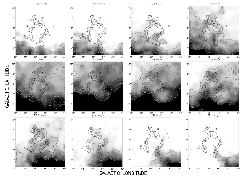
Figure 10: The $\lambda$21 cm HI-intensities in the area of G65.2+5.7 for the velocity range from $\rm-20\leavevmode\nobreak\ km\leavevmode\nobreak\ s^{-1}$ to 40 km s^-1, averaged over five consecutive channels ($\sim$5 km s^-1). The central LSR velocities are indicated above each panel. The grey-scale ranges between 40 and 300 K km s^-1. White contours are shown from 80 K km s^-1 (except for the 2.1 km s^-1 map, which starts at 100 k km s^-1) and increases in steps of 40 K km s^-1. The $\lambda$6 cm total intensities smoothed to $18\arcmin$ are superimposed as contours in black. The northern shell is located at about $67\degr$ longitude and the southern shell at about $64\degr$.

When rotating the E-vectors at $\lambda$11 cm in the same way as at $\lambda$6 cm, magnetic directions that differ up to $80\degr$ from a tangential orientation direction imply values of RM of the order of 150 rad m^-2 for the $\lambda$11 cm data to agree with a tangential magnetic field direction. This large RM disagrees with the $\lambda$6 cm data. However, as stated above, the observed level of the $\lambda$11 cm polarized emission is too low to be unaffected by unrelated Galactic large-scale emission. This needs to be taken into account before calculating any RM for G65.2+5.7, but we have insufficient information to do this. Clearly, we require observations at wavelengths shorter than $\lambda$6 cm of sufficiently high angular resolution to calculate the RM properties of G65.2+5.7 in combination with our $\lambda$6 cm data and thus contain the suggested tangential magnetic field orientation along its southern shell.

We can estimate the magnetic field strength in the southern shell by assuming energy equipartition between the magnetic field and electrons and protons in the SNR-shell using the formula by Fürst & Reich (2004), where the radius of a source is replaced by the volume V to deal with a shell section

$$B_{\min}\approx 175\cdot\Phi\,\mbox{}^{-2/7}\cdot V(pc^{3})\,\mbox{}^{-2/7}\cdot d(kpc)\,\mbox{}^{4/7}\cdot S_{1GHz}(Jy)\,\mbox{}^{2/7}$$ (1)

We extrapolated the integrated $\lambda$6 cm flux density without compact sources for the southern shell section centred on $\rm\alpha_{2000}=19^{h}33^{m}$, $\delta_{2000}=30\degr$ ($4\degr$ in $\alpha$, $1\degr$ in $\delta$) of $4.0$ Jy to $8.8$ Jy at 1 GHz for the error-weighted mean spectral index from TT-plots corresponding to $\alpha=-0.50$. We estimated the thickness of the southern shell from our highest angular resolution data at $\lambda$11 cm to be about 10% of the radius, or about 2.3 pc. For a distance of 0.8 kpc, we calculated a volume of the southern shell region of about $\rm 6500\leavevmode\nobreak\ pc^{3}$. The estimated equipartition magnetic field $\rm B_{min}$ is about $23\leavevmode\nobreak\ \mu$G for a filling factor $\Phi$ = 1, although this is a lower limit. In case of a highly filamentary shell, such as G65.2+5.7, a filling factor of $\Phi$ = 0.1 may be more appropriate, which would increase $\rm B_{min}$ to $45\leavevmode\nobreak\ \mu$G.

Another approach to estimating equipartition magnetic fields in SNRs was described by Foster (2005). This method results in a magnetic field strength of $\rm B\sim 36\leavevmode\nobreak\ \mu$G for $\alpha=-0.50$ over a frequency range of $\rm\nu_{min,max}=0.1-100\leavevmode\nobreak\$GHz, a line-of-sight extension of the radio-emitting region of 50 pc, and a radio intensity of the southern shell of $\rm I_{\nu}=0.2\times 10^{-18}ergs^{-1}cm^{-2}Hz^{-1}sr^{-1}$. We conclude that the magnetic field of the southern shell has a strength of between $\rm 20\leavevmode\nobreak\ and\leavevmode\nobreak\ 50\leavevmode\nobreak\ \mu$G.

3 Discussion

The radio properties of G65.2+5.7 show a number of similarities with another bilateral SNR G156.2+5.7 (Reich et al. 1992; Xu et al. 2007), which also has the lowest surface brightness of all known SNRs with a surface brightness of $\rm\Sigma_{1GHz}=5.8\times 10^{-23}$ W$\rm m^{-2}Hz^{-1}sr^{-1}$ at l GHz. The surface brightness of G65.2+5.7 is about $\rm\Sigma_{1GHz}=1.3\times 10^{-22}$ W$\rm m^{-2}Hz^{-1}sr^{-1}$, just about twice that of G156.2+5.7. Both SNRs are located outside the Galactic plane and at a similar distance of 800 pc or 1 kpc, although the shape of G65.2.+5.7 is more elliptical and its size is about 50% larger, possibly indicating that it is a more evolved object. Both are very bright in X-rays. The symmetry axis of both objects shows a large inclination relative to the Galactic plane, which has been taken as evidence that the ambient magnetic field has a similar inclination. The WMAP 22.8 GHz polarization data at an angular resolution of $2\degr$ in Fig. 7 indicate that the magnetic field is aligned almost parallel to the Galactic plane up to about $6\aas@@fstack{\circ}5$ latitude. Above $6\aas@@fstack{\circ}5$ latitude, the direction is less clearly defined. Of course, the WMAP data show the integrated polarization along the line-of-sight and local deviations in the magnetic field might be possible.

Some differences between G65.2+5.7 and G156.2+5.7 exist in their polarization properties. At $\lambda$6 cm and $\lambda$11 cm G156.2+5.7 has a higher fractional polarization. Depolarization along the outer shell of G65.2+5.7 seems to support the classification of a “thermal composite”, based on X-ray data, where a dense outer shell causes absorption of X-ray emission and strong depolarization (Shelton et al. 2004).

Orlando et al. (2007) presented simulations of the bilateral morphology of SNRs caused by density gradients in the interstellar medium or a gradient in the ambient magnetic field perpendicular to the radio shell. Smooth gradients are probably a simplification of the true conditions. However, we note that the intensity differences between the two arcs of the shell of G65.2+5.7 seem to agree with some of the simulations by Orlando et al. (2007) (their Fig.7, panels A and B), in which quasi-parallel particle injection was assumed and the viewing angle was perpendicular to both $\langle B\rangle$ and the gradients of either density or magnetic field strength. Slanting similar radio arcs were produced if the gradient was perpendicular to $\langle B\rangle$. In the quasi-perpendicular case, Orlando et al. (2007) found a bilateral shape when the gradient of the ambient $\langle B\rangle$ or density was parallel to $\langle B\rangle$. The symmetry axis of the SNR is always aligned with the gradient of density or the magnetic field. As indicated by the WMAP total intensity map (Fig. 7) or $\rm H_{\alpha}$ data (Fig. 13, right panel), thermal emission is evident along the northern and southern shell, and more smooth in the north than in the south. In addition to the general density gradient in the direction of Galactic latitude, this indicates a density difference in the direction of longitude, which results in compression differences in the interacting SNR shell and to a brightness difference as observed.

3.1 Analysis of HI-observations

Kalberla et al. (2005) published the Leiden/Argentina/Bonn (LAB) $\lambda$21 cm survey of neutral hydrogen, which covers the velocity range from $\rm-450\leavevmode\nobreak\ km\leavevmode\nobreak\ s^{-1}$ to $\rm+400\leavevmode\nobreak\ km\leavevmode\nobreak\ s^{-1}$ with a velocity resolution of $\rm 1.3\leavevmode\nobreak\ km\leavevmode\nobreak\ s^{-1}$. The HPBW of the survey was $0\aas@@fstack{\circ}6$, spectra were taken every $0\aas@@fstack{\circ}5$ and the r.m.s. brightness-temperature noise was about $\rm 0.07-0.09\leavevmode\nobreak\ K$.

A fully sampled HI-survey was also carried out with the DRAO 26-m telescope by Higgs et al. (2005). We found no significant difference between these two surveys, except that the DRAO HI-survey does not cover the very northern part of the SNR. Our HI-mass calculation is thus based on the LAB survey.

We extracted the HI-data of the G65.2+5.7 region from the LAB survey data-cube in the velocity range between $\rm-20\leavevmode\nobreak\ km\leavevmode\nobreak\ s^{-1}$ and $\rm 40\leavevmode\nobreak\ km\leavevmode\nobreak\ s^{-1}$. The 0.8 kpc distance corresponds to a velocity range $\rm 0-10\leavevmode\nobreak\ km\leavevmode\nobreak\ s^{-1}$ according to the Galactic rotation model given by Fich et al. (1989) of $\rm R_{0}=8.5\leavevmode\nobreak\ kpc$ and $\rm\Theta_{0}=220\leavevmode\nobreak\ km\leavevmode\nobreak\ s^{-1}$. Figure 10 displays the HI distribution after averaging five consecutive channels ($\rm\sim\leavevmode\nobreak\ 5\leavevmode\nobreak\ km\leavevmode\nobreak\ s^{-1}$) within the velocity interval from $-20$ to $\rm 40\leavevmode\nobreak\ km\leavevmode\nobreak\ s^{-1}$. The central velocity of each image is indicated at the top. Contours of $\lambda$6 cm total intensity (smoothed to $18\arcmin$) are superimposed to indicate the region of G65.2+5.7.

Although HI-fluctuations are visible across the entire field, we note signs of possible SNR interaction with the HI-gas in the images centered on $\rm v=-3.1\leavevmode\nobreak\ km\leavevmode\nobreak\ s^{-1}$, $\rm 2.1\leavevmode\nobreak\ km\leavevmode\nobreak\ s^{-1}$, and $\rm v=7.2\leavevmode\nobreak\ km\leavevmode\nobreak\ s^{-1}$. The northern shell correlates with the lower velocity maps, while the southern shell correlates with the $\rm 7.2\leavevmode\nobreak\ km\leavevmode\nobreak\ s^{-1}$ cloud. This may indicate that the northern shell is on the near side, or expands towards us, while the southern shell is on the far side or expands away from us.

In Fig. 11, we present the result for the integrated HI column densities over the velocity range $-5$ to $\rm 10\leavevmode\nobreak\ km\leavevmode\nobreak\ s^{-1}$. We integrated HI column densities over the velocity range $\rm-5\leavevmode\nobreak\ to\leavevmode\nobreak\ 10\leavevmode\nobreak\ km\leavevmode\nobreak\ s^{-1}$, and subtracted the large-scale diffuse emission using the ’unsharp-masking’ procedure described by Sofue & Reich (1979). A weak HI shell with an angular diameter of about 4$\degr$ is visible at the outer periphery of the radio continuum shell of SNR G65.2+5.7.

If a physical association exists, we would calculate the column density for the shell to be $\rm 2\leavevmode\nobreak\ \times\leavevmode\nobreak\ 10^{20}\leavevmode\nobreak\ cm^{-2}$. Assuming a thickness of the shell of 20% for a 2$\degr$ radius, this corresponds to a swept-up mass of about 1400 M$\odot$. The average density in the HI-shell is then about $\rm 1.2\leavevmode\nobreak\ cm^{-3}$. If this mass of neutral gas was originally uniformly distributed within a sphere of radius 2$\degr$, the pre-explosion ambient density would have been $\rm 0.6\leavevmode\nobreak\ cm^{-3}$, which is comparable to the value of $\rm 0.4\leavevmode\nobreak\ cm^{-3}$ estimated by Mason et al. (1979) for the X-ray emitting region. These densities are reasonable for a distance of $\sim$80 pc away from the Galactic plane.

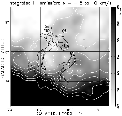
Figure 11: Integrated HI-intensities for the velocity range from $\rm-5\leavevmode\nobreak\ km\leavevmode\nobreak\ s^{-1}$ to 10 km s^-1 superimposed on with $\lambda$6 cm contours smoothed to $18\arcmin$. White contours for HI intensities are shown from 400 K km s^-1 and run in steps of 100 K km s^-1.

3.2 Comparison with observations from other bands

Figure 12: Superposition of an [O III] image (Boumis et al. 2004) with $\lambda$11 cm total intensity contours. The $\lambda$11 cm map has the same levels as shown in Fig. 2 but the compact sources were subtracted.

We show contours of $\lambda$11 cm total intensities of G65.2+5.7 superposed on an [O III] emission image by Boumis et al. (2004) in Fig. 12. The radio filaments are highly correlated with the [O III] filaments, which trace the fast SNR shock, except for the northwestern more diffuse part of the SNR. In this area, the SNR shock front seems to be distorted resulting in a less compressed magnetic field and a reduced efficiency in particle acceleration. We note that in some regions enhanced radio filamentary emission is seen without any corresponding optical emission. The magnetic fields might be stronger and/or the temperatures/densities lower in these bright radio filaments. This seems to be consistent with the measured incomplete cooling regions of G65.2+5.7 (Mavromatakis et al. 2002), which means that at least parts of the SNR are still in an adiabatic phase.

The G65.2+5.7 image ($\rm 0.14-0.284\leavevmode\nobreak\ keV$) from the ROSAT soft X-ray all-sky survey (Snowden et al. 1997) is shown in Fig. 13 (left panel) with contours of $\lambda$11 cm total intensity superimposed. The radio contours trace the outer SNR shock and clearly define an outer boundary of the X-ray emission. With its centrally filled X-ray thermal emission, G65.2+5.7 has been classified as a “thermal composite” SNR. Shelton et al. (2004) reviewed the evolution of “thermal composite” SNRs: A dense outer shell develops when the SNR enters the cooling phase, while the strong centrally peaked thermal X-ray emission may be explained by thermal conduction behind radiative shocks (Cox et al. 1999) and/or by the evaporation of interstellar clumps (White & Long 1991). More studies are needed to develop a detailed scenario of the evolution.

We show $\lambda$11 cm contours superposed on a $\rm H_{\alpha}$ image of G65.2+5.7 (Finkbeiner 2003) in Fig. 13 (right panel). A good correlation exists between the radio structures and enhanced $\rm H_{\alpha}$ emission, in particular along the southern shell. We estimate the thermal electron density within the southern shell using the observed emission measure (EM); this is defined as the integral of the square of electron density of the source along the line-of-sight l, $\rm EM=n_{e}^{2}$ $l$, and related to the $\rm H_{\alpha}$ intensity by

$$EM=2.75T_{4}^{0.9}I_{\rm H\alpha}\exp\left(\tau\right),$$ (2)

where $EM$ is in units of pc cm^-6, $I_{\rm H\alpha}$ is the H$\alpha$ intensity in Rayleigh, and the optical depth $\tau$ could be written in units of the product of $\rm E(B-V)$ magnitudes of reddening and 2.44 according to Finkbeiner (2003).

Assuming an electron temperature of 10000 K for the thermal gas and given an $\rm H_{\alpha}$ intensity of 18 Rayleigh for the southern filament by filtering out the diffuse emission, we obtained an EM of about 145 pc cm^-6 for a reddening $\rm E(B-V)$ of 0.44 (Schlegel et al. 1998). We then obtained an electron density $\rm n_{e}$ of between 38 cm^-3 and 22 cm^-3 for a thickness of between 0.1 pc and 0.3 pc. For the equipartition magnetic fields of $20\leavevmode\nobreak\ \mu$G to $50\leavevmode\nobreak\ \mu$G (filling factor 0.1), we may then calculate RMs ranging between 70 rad m^-2 and 245 rad m^-2 for the range of filament thicknesses and magnetic fields. We recall that for the case of a tangential magnetic field, the $\lambda$6 cm polarization angles constraint is about RM $\leq\rm 70\leavevmode\nobreak\ rad\leavevmode\nobreak\ m^{-2}$.

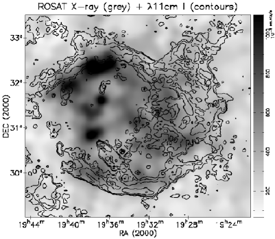
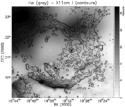
Figure 13: Superimposed images of SNR G65.2+5.7. Left: ROSAT X-ray emission (Snowden et al. 1997) (grey-scale) smoothed to $10\ arcmin$ angular resolution overlaid with $\lambda$11 cm total intensity contours . Right: $\rm H_{\alpha}$ map taken from Finkbeiner (2003) (grey-scale) overlaid with $\lambda$11 cm contours. Contour levels are as in Fig. 2. Note that compact sources were removed from the $\lambda$11 cm data shown here.

We also investigated the distribution of CO-emission from the “Composite CO-Survey” (Dame et al. 1987) for the SNR region, but found no evidence of any associated emission.

4 Summary

We have presented high sensitivity maps of the SNR G65.2+5.7 for total and polarized intensities at $\lambda$6 cm and $\lambda$11 cm. The spectral index of the integrated flux densities was found to be $\alpha=-0.58\pm 0.07$, which is consistent with the value obtained by Reich et al. (1979). The distribution of spectral indices shows some variation, although within the error margins of the spectral index obtained for the integrated emission.

Strong polarized emission is observed from the southern filament of G65.2+5.7, where a high percentage polarization around 50% at $\lambda$6 cm indicates the presence of a strong regular magnetic field component. Clear depolarization along its outer rim is seen at $\lambda$11 cm. The polarized emission at $\lambda$11 cm and $\lambda$6 cm are affected by a different amount of depolarization as well as confusion from diffuse Galactic polarized emission.

G65.2+5.7 is a faint large-diameter shell-type SNR with an exceptional low surface brightness in the radio range (Reich et al. 1979), but otherwise no unusual properties, e.g. no spectral bend as SNR S147 (Xiao et al. 2008). Except for possibly a few areas, G65.2+5.7 has almost entered the cooling phase. The strong depolarization along the outer SNR shell seems to support the classification of G65.2+5.7 as a rare example of a “thermal composite” SNR based on X-ray data.