Reconstructing 3-colored grids from
horizontal and vertical projections is NP-hard

Abstract

We consider the problem of coloring a grid using $k$ colors with the restriction that in each row and each column has an specific number of cells of each color. In an already classical result, Ryser obtained a necessary and sufficient condition for the existence of such a coloring when two colors are considered. This characterization yields a linear time algorithm for constructing such a coloring when it exists. Gardner et al. showed that for $k\geq 7$ the problem is NP-hard. Afterward Chrobak and Dürr improved this result, by proving that it remains NP-hard for $k\geq 4$. We solve the gap by showing that for $3$ colors the problem is already NP-hard. Besides we also give some results on tiling tomography problems.

1 Introduction

Tomography consists of reconstructing spatial objects from lower dimensional projections, and has medical applications as well as non-destructive quality control. In the discrete variant, the objects to be reconstructed are discrete, as for example atoms in a crystaline structure, see [1].

One of the first studied problem in discrete tomography involves the coloring of a grid, with a fixed number of colors with the requirement that each row and each column has a specific total number of entries of each color.

More formally we are given a set of colors $\cal C$, and an $m\times n$ matrix $M$, whose items are elements of $\cal C$. The projection of $M$ is a sequence of vectors $r^{c}\in{\mathbb{N}}^{m},s^{c}\in{\mathbb{N}}^{n}$, for $c\in\cal C$, where

$$r^{c}_{i} =|\{j:M_{ij}=c\}|, s^{c}_{j} =|\{i:M_{ij}=c\}|.$$

In the reconstruction problem, we are given only a sequence of vectors satisfying for $1\leq i\leq m$, $1\leq j\leq n$, $c\in\cal C$,

$$\sum_{c}r^{c}_{i} =n, \sum_{c}s^{c}_{j} =m, \sum_{i}r^{c}_{i} =\sum_{j}s^{c}_{j},$$ (1)

and the goal is to compute a matrix $M$ that has the given projections. If there are $k=|{\cal C}|$ colors, we call it the $k$-color Tomography Problem.

It was known since long time, that for 2 colors, the problem can be solved in polynomial time [8]. Ten years ago it was shown that the problem is NP-hard for 7 colors [5]. By NP-hardness, we mean that the decision variant — deciding whether a given instance is feasible, i.e. admits a solution — is NP-hard. Shortly after this proof was improved to show NP-hardness for 4 colors, leaving open the case when $|{\cal C}|=3$ [2]. This paper closes the gap, by showing that for 3 colors already the problem is NP-hard.

Just to fix the notation, for $|{\cal C}|=2$ we denote the colors as black and white, and use symbols $B,W$. For $|{\cal C}|=3$ we denote the colors as red, green and yellow and use symbols $R,G,Y$. Notice that we can think white and yellow as ground colors in the $2$ and $3-$color problem, respectively. Thus when we denote the instance of the tomography problem, we sometimes omit the white or yellow projections as they are redundant. In addition for a 2-color instance $(r^{B},s^{B})$ we omit the superscript when the context permits it.

First we recall some well known facts about the 2-color tomography problem.

Lemma 1 ([8])

Let $(r,s)$ be a feasible instance of the 2-color tomography problem. Let $I$ be some set of rows, and $J$ be some set of columns. If

$$\sum_{i\in I}r_{i}-\sum_{j\not\in J}s_{j}=|I\times J|,$$ (2)

then every solution to the instance will be all black in $I\times J$ and all white in $\overline{I}\times\overline{J}$.

Proof: The sets $I$,$J$ divide the grid into four parts, $I\times J$, $I\times\overline{J}$, $\overline{I}\times J$ and $\overline{I}\times\overline{J}$. The value $\sum_{i\in I}r_{i}$ equals the number of black cells in the first two parts, and $\sum_{j\not\in J}s_{j}$ the number of black cells in the second and last part. So the difference is the number of black cells in $I\times J$ minus the number of black cells in $\overline{I}\times\overline{J}$. So when (2) holds, the first part must be all black and the last part all white.     $\Box$

Before stating the next lemma, we need to introduce some notation about vectors. The conjugate of a vector $s\in\{0,1,\ldots,m\}^{n}$ is defined as the vector $s^{*}\in\{0,1,\ldots,n\}^{m}$ where $s^{*}_{i}=|\{j:s_{j}\geq i\}|$. There is a very simple graphical interpretation of this. Let be an $m\times n$ matrix $M$, such in column $j$, the first $s_{j}$ cells are colored black and the others are colored white. Then the conjugate of $s$ is just the row projection of $M$, see figure 1.

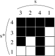
Figure 1: Example of a vector $s$ and its conjugate $s^{*}$.

Note that $s^{*}$ is always a non-increasing vector. If in addition $s$ is non-increasing we have that $(s^{*})^{*}=s$ since in this case $s^{*}_{i}=\max\{j:s_{j}\geq i\}$ and $s^{*}_{i}\geq j$ if and only if $s_{j}\geq i$.

For every $s,t\in\mathbb{N}^{n}$ we say that $s$ dominates $t$, denoted $s\succeq t$, if $\sum_{j=1}^{\ell}s_{j}\geq\sum_{j=1}^{\ell}t_{j}$ for every $1\leq\ell\leq n$. For any $0\leq k\leq n$ we define the set ${\cal X}_{n,k}:=\{x\in\{0,1\}^{n}:\sum x_{i}=k\}$. Clearly $\succeq$ defines a partial order on ${\cal X}_{n,k}$, and we show now that it has a small depth.

Lemma 2 ([2])

Let $n,k$ be two integers with $0\leq k\leq n$. Suppose we have a strictly increasing sequence

$$b^{0}\prec b^{1}\prec\ldots\prec b^{q},$$

of vectors from ${\cal X}_{n,k}$. Then $q\leq k(n-k)$.

Proof: For each vector $\alpha\in{\cal X}_{n,k}$ we associate the number $\varphi(\alpha)$ defined by $\varphi(\alpha)=\sum_{\ell=1}^{n}\sum_{i=1}^{\ell}\alpha_{i}$.

If $\alpha\prec\beta$ then $\sum_{j=1}^{\ell}\alpha_{j}\leq\sum_{j=1}^{\ell}\beta_{j}$ for every $1\leq\ell\leq n$ and the inequality is strict for at least one $\ell$. We conclude that $\alpha\prec\beta$ implies $\varphi(\alpha)<\varphi(\beta)$.

Therefore the vectors with extreme values for $\varphi$ are $\alpha=(0,\ldots,0,\underbrace{1,\ldots,1}_{k})$ and $\beta=(\underbrace{1,\ldots,1}_{k},0,\ldots,0)$. Since $\varphi(\alpha)=k(k-1)/2$ and $\varphi(\beta)=k(k-1)/2+k(n-k)$, this concludes the proof.     $\Box$

A well-known characterization of the feasible instances of the 2-color tomography problem can be expressed using dominance.

Lemma 3 ([8])

Let $(r,s)$ be an instance of the 2-color tomography problem, such that $r$ is non-increasing. Then $(r,s)$ is feasible if and only if $r\preceq s^{*}$. Moreover if $r=s^{*}$, then there is a single solution, namely the realization having the first $s_{j}$ cells of column $j$ colored black, and the others white.

There is a very simple graphical interpretation of this. Again let $M$ be a matrix where in column $j$ the first $s_{j}$ cells are colored black and the remaining cells white. Then the row projection of $M$ is $s^{*}$, and if $s^{*}=r$ we are done. Now if $s^{*}\neq r$, then some of the black cells in $M$ have to be exchanged with some white cells in the same column but a lower row. These operations transform the matrix in such a way, that the new row projection is dominated by $s^{*}$. So if $s^{*}$ does not dominate $r$, then there is no solution to the instance.

2 The gadget

The gadget depends on some integers $n,k,u,v$ with $1\leq k,u,v\leq n$ and $u\neq v$ as well as on two vectors $\alpha,\beta\in{\cal X}_{n,k}$. It is defined as the instance of $n$ rows, and $2n+2$ columns with the following projections for $1\leq i,j\leq n$

$$r^{R}_{i} =\left\{\begin{array}[]{ll}i+1&\mbox{if }i\in\{u,v\}\\ i&\mbox{otherwise}\end{array}\right. r^{G}_{i} =\left\{\begin{array}[]{ll}i&\mbox{if }i\in\{u,v\}\\ i+1&\mbox{otherwise}\end{array}\right.$$

$$s^{R}_{j} =n-j+\alpha_{j} s^{G}_{j} =0$$

$$s^{R}_{n+1} =1 s^{G}_{n+1} =n-1$$

$$s^{R}_{n+2} =n-k+1 s^{G}_{n+2} =k-1$$

$$s^{R}_{n+2+j} =0 s^{G}_{n+2+j} =n-j+1-\beta_{j}.$$

Lemma 4

If the instance above is feasible then $\alpha\preceq\beta$. Moreover, if $\alpha=\beta$ then the instance is feasible if and only if $\alpha_{u}+\alpha_{v}\geq 1$.

Proof: Assume the instance is feasible, we will show that this implies $\alpha\preceq\beta$. Consider the yellow projection vectors $r^{Y}=2n+2-r^{R}-r^{G}$ and $s^{Y}=n-s^{R}-s^{G}$. We have that $r^{Y}_{i}=2(n-i)+1$ for $1\leq i\leq n$. Note that $r^{Y}$ is a non-increasing vector. Similarly, we obtain that $s^{Y}_{j}=j-\alpha_{j}$ and $s^{Y}_{n+2+j}=j-1+\beta_{j}$, for $1\leq j\leq n$, and $s^{Y}_{n+1}=s^{Y}_{n+2}=0$. The conjugate of the column yellow projections is a vector $(s^{Y})^{*}$ with

$$(s^{Y})^{*}_{i}=2(n-i)+1-\alpha_{i}+\beta_{i}.$$

Then clearly $r^{Y}\preceq(s^{Y})^{*}$ if and only if $\alpha\preceq\beta$. By assumption the 3-color instance $(r^{R},r^{G},r^{Y},s^{R},s^{G},s^{Y})$ is feasible, therefore the 2-color instance $(r^{Y},s^{Y})$ is feasible as well — where yellow is renamed as black — which by Lemma 3 implies $r^{Y}\preceq(s^{Y})^{*}$ and therefore also $\alpha\preceq\beta$. This shows the first part of the lemma.

Now assume that the instance has a solution, and $\alpha=\beta$. The $n\times(2n+2)$ grid is divided into 3 parts (see figure 2): into an $n\times n$ block (called RY-block), a $n\times 2$ rectangle (called 2-column translator) and another $n\times n$ block (called GY-block). Again every block is sub-divided into an upper triangle, a diagonal and a lower triangle.

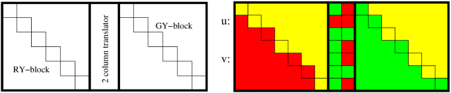
Figure 2: The structure of the gadget (left) and a realization (right) for $n=7$, $k=3$, $u=2$, $v=5$ and $\alpha=\beta=(0,0,1,0,1,1,0)$.

Since $\alpha=\beta$, we have $r^{Y}=(s^{Y})^{*}$. So by Lemma 3 any solution must color in yellow the $s^{Y}_{j}$ first cells in every column $j$, and no other cell. In particular it means that the lower triangle of the RY-block must be red, the lower triangle of the GY-block must be green, and both upper triangles have to be yellow.

Also on the first diagonal, the cell $(i,i)$ has to be red if $\alpha_{i}=1$ and yellow otherwise. On the second diagonal, the cell $(n+2+i,i)$ must be yellow if $\alpha_{i}=1$ and green otherwise.

What can we say about the colors of the translator? If $\alpha_{u}=\alpha_{v}=0$, then the cells $(n+1,u),(n+2,u),(n+1,v),(n+2,v)$ have to be all red to satisfy the row projections. This contradicts the column projection $s^{R}_{n+1}=1$, and hence the instance is not feasible.

Conversely, assume $\alpha_{u}+\alpha_{v}\geq 1$. We will color the cells of the translator in a manner that respects the required projections. If $i\not\in\{u,v\}$ and $\alpha_{i}=1$ — that is $(i,i)$ is red — we color the cells $(n+1,i),(n+2,i)$ in green. If $i\not\in\{u,v\}$ and $\alpha_{i}=0$, we color the cell $(n+1,i)$ in green and $(n+2,i)$ in red.

Without loss of generality assume that $\alpha_{u}=1$. Hence $(u,u)$ is red and we color $(n+1,u)$ in green and $(n+2,u)$ in red. We color $(n+1,v)$ in red. In addition we color $(n+2,v)$ in red if $\alpha_{v}=0$ and in green otherwise. It can be verified that the coloring defined above is a solution to the instance, which concludes the proof of the lemma.     $\Box$

3 The reduction

In this section we will construct a reduction from Vertex Cover to 3-color tomography. We basically use the same approach than in [2], but with a different gadget.

Vertex Cover is a well known intractable problem, indeed one of the first 21 problems shown to be NP-complete by Karp [6].

Vertex Cover Problem

• Input: a graph $G=(V,E)$ and an integer $k$.

• Output: a set $S\subseteq V$ of size $|S|=k$ such that for every $(u,v)\in E$, $u\in S$ or $v\in S$.

Given an instance $(G,k)$ of Vertex Cover, we construct an instance $(r^{R},r^{B},s^{R},s^{B})$ of the 3-color tomography problem which is feasible if and only if the former instance has a solution. Without loss of generality we assume that $k\leq n-2$.

Let be $n=|V|,m=|E|$, and $N=k(n-k)(m-1)+1$. We denote the $m$ edges as $E=\{e_{0},e_{1},\ldots,e_{m-1}\}$, and the $n$ vertices as $V=\{1,2,\ldots,n\}$. We define an instance with $N(n+1)+1$ rows and $N(n+2)+n$ columns.

For row $p=1,\ldots,N(n+1)+1$, let

$$x =\lfloor(p-1)/(n+1)\rfloor$$

$$i =(p-1)\bmod(n+1).$$

We think the set of rows as divided into $N$ blocks of $n+1$ rows each, and a last block with a single row. We have $x$ as the block index and $i$ the row index relative to the block, with $0\leq i\leq n$. Let $t=x\bmod m$ and consider the edge $e_{t}=(u,v)$. We define the projections

$$r^{R}_{p} =x(n+2)+\left\{\begin{array}[]{ll}n-k&\mbox{if }x<N\mbox{ and }i=0\\ 0&\mbox{if }x=N\mbox{ and }i=0\\ i+1&\mbox{if }i\in\{u,v\}\\ i&\mbox{if }i\in\{1,\ldots,n\}\setminus\{u,v\}\\ \end{array}\right.$$

$$r^{G}_{p} =(N-x-1)(n+2)+\left\{\begin{array}[]{ll}n+2&\mbox{if }x=0\mbox{ and }i=0\\ n+2+k&\mbox{if }x>0\mbox{ and }i=0\\ i&\mbox{if }i\in\{u,v\}\\ i+1&\mbox{if }i\in\{1,\ldots,n\}\setminus\{u,v\}.\\ \end{array}\right.$$

In the same manner, for column $q=1,\ldots,N(n+2)+n$, let

$$y =\lfloor(q-1)/(n+2)\rfloor$$

$$j =((q-1)\bmod(n+2))+1.$$

The reason for defining $j$ this way, is that if cell $(p,q)$ is part of an RY-block or an GY-block, then $(i,j)$ will be the relative position inside the block with ranges $1\leq i,j\leq n$. Similarly as for the rows, we think the set of columns as divided into $N$ blocks with $n+2$ columns each and a last block with only $n$ columns. Again, we have $y$ as the block index, and $j$ as the column index relative to a block with $1\leq j\leq n+2$. For block $0\leq y\leq N-1$ we define the red column projections as

$$s^{R}_{q} =(N-y-1)(n+1)+1+\left\{\begin{array}[]{ll}n-j+1&\mbox{if }j\in\{1,\ldots,n\}\\ 1&\mbox{if }j=n+1\\ n-k+1&\mbox{if }j=n+2,\\ \end{array}\right.$$

For $y=N$ we set $s^{R}_{q}=0$, for each $j=1,\ldots,n$. Similarly, for $y=0$ the green column projections are

$$s^{G}_{q} =\left\{\begin{array}[]{ll}0&\mbox{if }j\in\{1,\ldots,n\}\\ n&\mbox{if }j=n+1\\ k&\mbox{if }j=n+2.\\ \end{array}\right.$$

and for $1\leq y\leq N$ they are defined as

$$s^{G}_{q} =(y-1)(n+1)+1+\left\{\begin{array}[]{ll}j&\mbox{if }j\in\{1,\ldots,n\}\\ n-1&\mbox{if }j=n+1\\ k-1&\mbox{if }j=n+2.\\ \end{array}\right.$$

Figure 3: The general structure of our reduction

Clearly this a polynomial time reduction. It remains to show the following theorem.

Theorem 1

The 3-color tomography instance is feasible if and only if the vertex cover instance is feasible.

Proof: For one direction of the statement, assume that the vertex cover instance is feasible, and let $b\in{\cal X}_{n,k}$ be the characteristic vector of a vertex cover of size $k$, i.e. $b_{i}=1$ if and only if $i$ belongs to the vertex cover.

We construct now a solution to the tomography instance. Consider the partitioning of the grid, as in figure 3. For convenience we refer to the source also as the $0$-th row translator and to the sink as the $(N+1)$-th row translator. The $j$-th cell of the $x$-th row translator is defined as $(x(n+1)+1,x(n+2)+j)$. We color the R-frame in red and the G-frame in green.

Let be any $1\leq j\leq n$. We color the $j$-th cell of the source in yellow if $b_{j}=1$ and in red otherwise. For $x=1,\ldots,N-1$ we color the $j$-cell of the $x$-th row translator in green if $b_{j}=1$ and in red otherwise. In the sink we color the $j$-th cell in green if $b_{j}=1$ and in yellow otherwise.

Now for block $x=0,\ldots,N-1$, consider the instance to the gadget defined by $\alpha=\beta=b$, and $u,v$ such that $(u,v)=e_{x\bmod m}$. By Lemma 4 it is feasible, since $b$ is a vertex cover and hence $b_{u}+b_{v}\geq 1$. Then we color the $(n+1)\times(2n+2)$ cells starting at $((x-1)(n+2)+1,(x-1)(n+1)+1)$ exactly as in the solution to the gadget. It is straightforward to check that this grid satisfies the required projections, and therefore the tomography instance is feasible.

For the converse, assume that the tomography instance has a solution. For every $x=1,\ldots,N$ we apply Lemma 1 for the red color and intervals $I=[x(n+1)+1,N(n+1)+1]$ and $J=[1,x(n+2)]$. We deduce that in the solution the R-frame must be all red, and all GY-blocks (and also the G-frame) must be free of any red. Similarly, we show that the G-frame must be all green, and all RY-blocks must be free of any green.

This implies that in the source, $k$ cells are yellow, and $n-k$ are red, in the row translators $k$ cells are green and $n-k$ red, and in the sink $k$ cells are green and $n-k$ yellow. We define the vectors $b^{0},b^{1},\ldots,b^{N}\in{\cal X}_{n,k}$, such that for all $1\leq j\leq n$ we have

• $b^{0}_{j}=1$ iff the $j$-th cell in the source is yellow,

• $b^{x}_{j}=1$ iff the $j$-th cell in the $x$-th row translator is green, for all $1\leq x\leq N$.

For $x=0,\ldots,N$, consider the part $P$ of the solution that is the intersection of rows $[x(n+1)+2,x(n+1)+n+1]$ and columns $[x(n+2)+1,x(n+2)+2n+2]$. We number the rows of $P$ from $1$ to $n$ and the columns from $1$ to $2n+2$. Let $(u,v)=e_{x\bmod m}$. By subtracting from the row projections the number of red and green cells in the frames, we deduce that row $1\leq i\leq n$ in $P$ contains $i+1$ red cells and $i$ green cells if $i\in\{u,v\}$ and $i$ red cells and $i+1$ green cells if $i\not\in\{u,v\}$.

We proceed similarly for the columns $n+1$ and $n+2$. By subtracting from the column projections the quantities that are in the frames, we deduce that column $n+1$ of $P$ contains one red cell, and $n-1$ green cells, and column $n+2$ contains $n-k+1$ red cells and $k-1$ green cells.

Column $x(n+2)+j$ for $1\leq j\leq n$ contains $n-j+1$ red cells that are not in the R-frame. Since GY-blocks are free of red, these cells must either be in the $x$-th row translator or in column $j$ of $P$. Note that the $j$-cell of the $x$-th row translator is red iff $b^{x}_{j}=0$. Therefore column $j$ of $P$ contains $n-j+b^{x}_{j}$ red cells and no green cell. Similarly column $n+2+j$ of $P$ contains $n-j+1-b^{x+1}_{j}$ green cells and no red cell.

This implies that $P$ is the solution to the gadget defined by $u,v,\alpha,\beta$ with $\alpha=b^{x}$ and $\beta=b^{x+1}$. Then by Lemma 4 we obtain that $b^{x}\preceq b^{x+1}$ and in general

$$b^{0}\preceq b^{1}\preceq\ldots\preceq b^{N}.$$

By the choice of $N$ and Lemma 2 there exists an $\ell$ such that

$$b^{\ell}=b^{\ell+1}=\ldots=b^{\ell+m}.$$

By Lemma 4, we have $b^{\ell}_{u}+b^{\ell}_{v}\geq 1$ for all $(u,v)\in\{e_{\ell},e_{\ell+1\bmod m},\ldots,e_{\ell+m-1\bmod m}\}=E$. Therefore $b^{\ell}$ encodes a vertex cover of size $k$, and this completes the proof.     $\Box$

4 Related problems

4.1 Edge-colored graphs with prescribed degrees

We can reduce the $3$-color tomography problem to a similar graph problem.

Finding edge-colored graphs with prescribed degrees

Let be a set of two colors $\{R,G\}$, and a vertex set $V$. We are given prescribed degrees $d^{R},d^{G}:V\rightarrow\mathbb{N}$ and have to find two disjoint edge sets $E^{R},E^{G}\subseteq V^{2}$ such that the graph $G(V,E^{R}\cup E^{G})$ has the required degrees, i.e. for all $v\in V$

$$d^{R}(v)=|\{u:(u,v)\in E^{R}\}| d^{G}(v)=|\{u:(u,v)\in E^{G}\}|.$$

Note that in contrast, finding an uncolored graph with given degree sequences can be solved in polynomial time, see for example [7].

Lemma 5

The problem of finding an edge-colored graph with prescribed degrees is NP-hard.

Proof: We reduce from the $3$-color tomography problem. Let $(r^{R},r^{G},s^{R},s^{G})$ be an $m\times n$-instance of the 3-color tomography problem. We set $k=n+m$, $V=\{1,\ldots,k\}$, and the following degrees, for $1\leq i\leq n$ and $1\leq j\leq m$

$$d^{R}(i) =r^{R}_{i}+n-1 d^{G}(i) =r^{G}_{i}$$

$$d^{R}(n+j) =s^{R}_{j} d^{G}(n+j) =s^{G}_{j}+m-1.$$

Now we show that the instance $(r^{R},r^{G},s^{R},s^{G})$ is feasible if and only if the instance $(d^{R},d^{G})$ is feasible. For one direction, assume that there is a solution $M$ to the 3-color tomography instance. We construct a solution $E^{R},E^{G}$ to the graph problem as follows. For any $1\leq i\leq n$ and $1\leq j\leq m$, if $M_{ij}=R$, then $(i,n+j)\in E^{R}$, if $M_{ij}=G$, then $(i,n+j)\in E^{G}$. Also for any $1\leq i<i^{\prime}\leq n$, we have $(i,i^{\prime})\in E^{R}$ and for any $1\leq j<j^{\prime}\leq m$, we have $(n+j,n+j^{\prime})\in E^{G}$. Now clearly $E^{R},E^{G}$ satisfy the required degrees.

For the converse, we define the quantity $\Phi=\sum_{i=1}^{n}d^{R}(i)-\sum_{j=1}^{m}d^{R}(n+j)$. By assumption (1) this value is $n(n-1)$. Since this value equals also

$$|E^{R}\cap\{1,\ldots,n\}^{2}|-|E^{R}\cap\{n+1,\ldots,n+m\}|,$$

there is a red edge between every pair of vertices $(i,i^{\prime})$ with $1\leq i<i^{\prime}<n$, and no edge between every pair of vertices $(n+j,n+j^{\prime})$ with $1\leq j<j^{\prime}\leq m$. Similarly we can show that there is a green edge between every pair of vertices $(n+j,n+j^{\prime})$ with $1\leq j<j^{\prime}\leq m$.

Now let $M$ be the $m\times n$ grid, with cell $(i,j)$ colored in red if $(i,n+j)\in E^{R}$, and in green if $(i,n+j)\in E^{G}$. By the degree requirements, $M$ is a solution to the 3-color tomography instance.     $\Box$

4.2 Tiling Tomography

Tiling tomography was introduced in [3], and it consists of constructing a tiling that satisfies some given row and column projections for each type of tiles we admit.

Formally a tile is a finite set $T$ of cells of the grid $\mathbb{N}\times\mathbb{N}$, that are 4-connected, in the sense that the graph $G(T,E)$ is connected for $E=\{((i,j),(i^{\prime},j^{\prime})):|i-i^{\prime}|+|j-j^{\prime}|=1\}$. By $T+(i^{\prime},j^{\prime})=\{(i+i^{\prime},j+j^{\prime}):(i,j)\in T\}$ we denote a copy of $T$ that is shifted $i^{\prime}$ units down and $j^{\prime}$ units to the right. We say that a set of tiles is feasible if they do not intersect. In addition we say that it tiles the $m\times n$ grid if its (disjoint) union equals the set of all grid cells, and we refer it as a tiling.

In the tiling tomography problem we are given a finite set of tiles ${\cal T}=\{T_{1},\ldots,T_{k}\}$, and vectors $r^{d}\in{\mathbb{N}}^{m},s^{d}\in{\mathbb{N}}^{n}$ for $1\leq d\leq k$. The goal is to compute a matrix $M\in\{0,1,\ldots,k\}$ such that the set

$$\bigcup_{1\leq d\leq k}\{T_{d}+(i,j):1\leq i\leq n,1\leq j\leq m\mbox{ such that }M_{ij}=d,\mbox{ for }1\leq d\leq k\}$$

is a tiling of the $m\times n$ grid, with the projections

$$r^{d}_{i} =|\{j:M_{ij}=d\}| s^{d}_{j} =|\{i:M_{ij}=d\}|.$$

By width and height of a tile $T$ we understand the size of the smallest intervals $I,J$ such that $T\subseteq I\times J$. This definition extends to set of tiles. A tile $T$ is said to be rectangular if for every $(i^{\prime},j^{\prime})$ such that $\{T,T+(i^{\prime},j^{\prime})\}$ is feasible, we have that the width of $\{T,T+(i^{\prime},j^{\prime})\}$ is at least twice the width of $T$ or the height of the set is at least twice the height of $T$.

It was conjectured in [3], that for $T_{1}$ being a single cell and $T_{2}$ a non-rectangular tile, the $\{T_{1},T_{2}\}$-tiling tomography problem is NP-hard. This question is still open and intriguing.

4.3 Rectangular tiles

Consider two rectangular tiles, $T_{1}$ being a $p_{1}\times q_{1}$ rectangle and $T_{2}$ a $p_{2}\times q_{2}$ rectangle, i.e. $T_{c}=\{0,\ldots,p_{c}-1\}\times\{0,\ldots,q_{c}-1\}$, for $c\in\{1,2\}$. What can be said about the complexity of the $\{T_{1},T_{2}\}$-tiling tomography problem?

If $\gcd(p_{1},p_{2})=d>1$, then clearly any solution $\bar{M}\in\{0,1,2\}^{m\times n}$ to a $\{T_{1},T_{2}\}$-tiling tomography instance $(r^{c},s^{c})$, must satisfy that if $\bar{M}_{ij}\neq 0$, then $i\bmod d=1$. Therefore the $\{T_{1},T_{2}\}$-tiling tomography problem can be reduced to the $\{T^{\prime}_{1},T^{\prime}_{2}\}$-tiling tomography problem, with $T^{\prime}_{1}$ being a $(p_{1}/d)\times q_{1}$ rectangle, and $T^{\prime}_{2}$ a $(p_{2}/d)\times q_{2}$ rectangle. We omit the formal reduction, which is straightforward.

From now on suppose that $\gcd(p_{1},p_{2})=\gcd(q_{1},q_{2})=1$. We distinguish the following cases, up to row-column symmetry.

• If $p_{1}=p_{2}=1$, that is the tiles are two horizontal bars of length $q_{1}$ and $q_{2}$, then the problem can be solved in polynomial time (Theorem 2). We use an idea already present in [4], where it is proven for $q_{1}=1$.

• If $p_{1}=q_{2}=1$ and $p_{2}=q_{1}=2$, then the tiles are called dominoes, and again the problem can be solved in polynomial time, although with a more involved algorithm [9].

• If $p_{1}=q_{2}=1$, $p_{2}\geq 2$ and $q_{1}\geq 3$ then the problem is open. The first author conjectures that the problem is NP-hard, while the other two conjecture that it could be solved in polynomial time with a similar approach as in [9].

• If $p_{1},q_{1}\geq 2$, then the problem is NP-hard (Theorem 3). In [3] the special case $p_{1}=q_{1}=2$, $p_{2}=q_{2}=1$ was related to the 3-color tomography problem, and it is therefore also NP-hard. We generalize this reduction in section 4.6

• If there is a third rectangular tile $T_{3}$, then for the tile set $\{T_{1},T_{2},T_{3}\}$ the problem is NP-hard, see section 4.7.

4.4 An algorithm for vertical bars

Theorem 2

The tiling tomography problem can be solved in polynomial time for two rectangular tiles of dimensions $p_{1}\times 1$ and $p_{2}\times 1$.

Proof: The algorithm is the simple greedy algorithm, as the one used in [4]. It iteratively stacks bars in the matrix.

Formally the algorithm is defined like this. We construct a matrix $A\in\{0,1,2\}^{m\times n}$ with the required projections. Initially $A$ is all $0$. We maintain a vector $v$ such that $v_{j}$ is the minimal $i$ such that $A_{i,j}\neq 0$, and $v_{j}=m+1$ if column $j$ of $A$ is all zero. Initially $v_{j}=m+1$ for all $1\leq j\leq n$. We also maintaing vectors $\bar{r}^{1},\bar{r}^{2},\bar{s}^{1},\bar{s}^{2}$, which represent the remaining projections. Initially they equal the given projections of the instance. The vectors $(v,\bar{r}^{1},\bar{r}^{2},\bar{s}^{1},\bar{s}^{2})$ define a more general tiling problem, where in every column $j$, only the first $v_{j}-1$ cells have to be tiled.

The algorithm: Let $i=\max v_{j}$. If $i=1$ we are done, and return $A$, if all vectors $\bar{r}^{1},\bar{r}^{2},\bar{s}^{1},\bar{s}^{2}$ are zero, and return “no solution” otherwise.

If $i>1$, let $i_{1}=i-p_{1}$ and $i_{2}=i-p_{2}$. If $\bar{r}^{1}_{i_{1}}=\bar{r}^{2}_{i_{2}}=0$, abort and return “no solution”. Otherwise let $c\in\{1,2\}$ such that $\bar{r}^{c}_{i_{c}}>0$. Let $j$ be a column with $v_{j}+1=i$ that maximizes $\bar{s}^{c}_{j}$. Then drop the bar $p_{c}\times 1$ in column $j$, i.e. set $A_{i_{c},j}=c$, and decrease $\bar{r}^{c}_{i_{c}}$ and $\bar{s}^{c}_{j}$. Repeat the whole step.

Clearly, if this algorithm produces a matrix, then it defines a valid tiling with the required projections. We have to show that if the instance has a solution, then the algorithm will actually find one. For this purpose, let be some step of algorithm such that the intermediate instance ${\cal I}:=(v,\bar{r}^{1},\bar{r}^{2},\bar{s}^{1},\bar{s}^{2})$ is feasible. The initial step could be a candidate. Let $M$ be a solution to it. Let $i=\max v_{j}$. If $i=1$, then $\bar{r}^{1},\ldots,\bar{s}^{2}$ are all zero, since the instance is feasible.

Let $i_{1}=i-p_{1}$ and $i_{2}=i-p_{2}$. We have that either $M_{i_{1},j}=1$ or $M_{i_{2},j}=2$ for every column $j$ satisfying $v_{j}=i$, since $M$ is a valid tiling. Therefore some of $\bar{r}^{1}_{i_{1}},\bar{r}^{2}_{i_{2}}$ must be non zero. Let $c,j$ be the values the algorithm chooses. Let ${\cal I^{\prime}}$ be the instance obtained after the iteration of the algorithm, that is $\bar{r}^{c}_{i_{c}},\bar{s}^{c}_{j}$ are decreased by $1$ and $v_{j}$ by $p_{c}$.

If $M_{i_{c},j}=c$, then $M^{\prime}$ which equals $M$ except for $M_{i_{c},j}=0$ is a solution to ${\cal I^{\prime}}$.

If $M_{i_{c},j}\neq c$, then by the projections, there must be a another column $k$ with $v_{k}=i$ and $M_{i_{c},k}=c$. We will now transform $M$ such that $M_{i_{c},j}=c$. Then we are in the case above and done.

By the choice of the algorithm we have $\bar{s}^{c}_{k}\leq\bar{s}^{c}_{j}$. By this inequality, there exists $i_{0}$ such that the total number of $c$’s below the row $i_{0}$ is the same in both column $j$ and column $k$. Take $i_{0}$ being the largest one satisfying that. By the choice of $i_{0}$ we have that $M_{i_{0},j}=c$ and $M_{i_{0},j}\neq c$. Since $M$ is a valid tiling, then the restriction to cells below $i_{0}$ in column $k$ is also a tiling and then $M_{i_{0},j}\neq 0$. We conclude that between $i_{0}$ and $i$ the number of 1’s and 2’s in column $j$ is the same as in column $k$. Then exchanging the parts of columns $j$ and $k$ in $M$ between $i_{0}$ and $i$, does not change the projections of $M$, and we obtain the required property $M_{i_{c},j}=c$.

Figure 4: Transforming a solution $M$ for $c=1$.

By the choice of the algorithm we have $s^{c}_{k}\leq s^{c}_{j}$. Now we claim that there is a row $i_{0}$ such between $i_{0}$ and $i$ the number of 1’s and 2’s in column $j$ is the same as in column $k$. Indeed, consider the largest $i_{0}$ such that the total number of $c$’s below the row $i_{0}$ is the same in both column $j$ and column $k$. It must be that $M_{i_{0},j}=c$ and $M_{i_{0},k}\neq 0$ since $M$ is a valid tiling. Then exchanging the parts of columns $j$ and $k$ in $M$ between $i_{0}$ and $i$, does not change the projections of $M$, and we obtain the required property $M_{i_{0},j}=c$.

$\Box$

4.5 A general NP-hardness proof structure

In the next section we will reduce the 3-color tomography problem to the tiling tomography problem for some fixed set of tiles $\cal T$. The proof uses a particular structure that we explain now.

Let $(r^{R},r^{G},r^{Y},s^{R},s^{G},s^{Y})$ be an instance to the 3-color tomography problem for an $m\times n$ grid. In the reduction we will choose constant size grid $\ell\times k$ — that we call a block — and three $\cal T$-tilings of it, that we denote $\bar{M}^{R},\bar{M}^{G},\bar{M}^{Y}$. There will be two requirements: Let $\bar{r}^{c,d},\bar{s}^{c,d}$ be the $T_{d}$-projections of the tiling $\bar{M}^{c}$ for $c\in\{R,G,Y\}$ and $d\in\{1,2\}$.

The first requirement is that the vectors $\{\bar{r}^{R,1},\bar{r}^{G,1},\bar{r}^{Y,1}\}$ are affine linear independent. The same requirement holds for the column projections $\{\bar{s}^{R,1},\bar{s}^{G,1},\bar{s}^{Y,1}\}$. This implies that every vector $r$ spanned by $\bar{r}^{R,1},\bar{r}^{G,1},\bar{r}^{Y,1}$, has a unique decomposition into $r=n_{R}\bar{r}^{R}+n_{G}\bar{r}^{G}+n_{Y}\bar{r}^{Y}$ for $n_{R}+n_{G}+n_{Y}=n$.

The reduction, consists of an $m\ell\times nk$ grid, and the projections $1\leq i\leq\ell$, $1\leq j\leq k$, $1\leq x\leq m$, $1\leq y\leq n$, $d\in\{1,2\}$

$$r^{d}_{x\ell-\ell+i} =\sum_{c}r^{c}_{x}\cdot\bar{r}^{c,d}_{i}$$

$$s^{d}_{yk-k+j} =\sum_{c}s^{c}_{y}\cdot\bar{s}^{c,d}_{j}$$

The idea is that the $m\ell\times nk$ is partitioned into $mn$ blocks of dimension $\ell\times k$. The second requirement is that in every solution $\bar{M}$ to the tiling instance, all blocks of $\bar{M}$, are either $\bar{M}^{R},\bar{M}^{G},\bar{M}^{Y}$ or blocks that have equivalent projections.

Lemma 6

The instance to the $\cal T$-tiling problem has a solution if and only if the instance to the 3-color tomography problem has a solution.

Proof: Let $M\in\{R,G,Y\}^{m\times n}$ be a solution to the 3-color tomography problem. We transform it into a matrix $\bar{M}\in\{0,1,2\}^{m\ell\times nk}$ by replacing each cell $(i,j)$ of $M$ by the $\ell\times k$ matrix $\bar{M}^{c}$ for $c=M_{ij}$. By construction, this is a solution to the tiling problem.

For the converse, suppose that there is a solution $\bar{M}$ to the tiling problem. By the second requirement, every block of $\bar{M}$ can be associated to one of the colors $\{R,G,Y\}$. We construct a matrix $M\in\{R,G,Y\}^{m\times n}$ such that $M_{xy}=c$ if the block $(x,y)$ of $\bar{M}$ is $\bar{M}^{c}$, or something projection equivalent.

Fix some arbitrary $1\leq x\leq m$. By the first requirement, the projections of the rows $x\ell-\ell+1,\ldots,x\ell$ have a unique decomposition into $n_{R}r^{R,1}+n_{G}r^{G,1}+n_{Y}r^{Y,1}$ with $n_{R}+n_{G}+n_{Y}=n$. By the definitions of the projections $n_{R}=r^{R}_{x},n_{G}=r^{G}_{x},n_{Y}=r^{Y}_{x}$, and then row $x$ of $M$ has the required projections. We proceed in the same manner for the columns and show that $M$ is a solution to the 3-color tomography instance.     $\Box$

4.6 An NP-hardness proof for two rectangular tiles

Theorem 3

The tiling tomography problem is NP-hard for two rectangular tiles of dimensions $p_{1}\times q_{1}$ and $p_{2}\times q_{2}$ with $\gcd(p_{1},p_{2})=\gcd(q_{1},q_{2})=1$ and $p_{1},q_{1}\geq 2$.

Proof: We apply Lemma 6 for $\ell=2p_{1}p_{2}$ and $k=2q_{1}q_{2}$. The 3 tilings of the $\ell\times k$ grid are depicted in figure 5, and defined formally as follows. The rows $I=\{1,\ldots,\ell\}$ and the columns $J=\{1,\ldots,k\}$ are partitioned into sets $I_{1},I_{2},I_{3},I_{4}$ and $J_{1},J_{2},J_{3},J_{4}$ defined as

$$I_{1} =\{1,\ldots,p_{2}\} J_{1} =\{1,\ldots,q_{2}\}$$

$$I_{2} =\{p_{2}+1,\ldots,p_{1}p_{2}\} J_{2} =\{q_{2}+1,\ldots,q_{1}q_{2}\}$$

$$I_{3} =\{p_{1}p_{2}+1,\ldots,p_{1}p_{2}+p_{2}\} J_{3} =\{q_{1}q_{2}+1,\ldots,q_{1}q_{2}+q_{2}\}$$

$$I_{4} =\{p_{1}p_{2}+p_{2}+1,\ldots,2p_{1}p_{2}\} J_{4} =\{q_{1}q_{2}+q_{2}+1,\ldots,2q_{1}q_{2}\}.$$

Then $\bar{M}^{R}$ is defined as the block tiling that covers $(I_{1}\cup I_{4})\times(J_{3}\cup J_{4})$ with $T_{2}$ and the rest with $T_{1}$, $\bar{M}^{G}$ is defined as the block tiling that covers $(I_{3}\cup I_{4})\times(J_{1}\cup J_{4})$ with $T_{2}$ and the rest with $T_{1}$, while $\bar{M}^{Y}$ is defined as a tiling using only $T_{1}$. These tilings are uniquely defined. Clearly the row $T_{1}$-projections of the 3 tilings are affine linear independent, so the first requirement of the construction is satisfied.

Figure 5: The 3 valid block tilings.

The second requirement follows from a sequence of observations. Let $\bar{M}$ be the solution to the tiling instance, obtained by reduction from a 3-color instance $(r^{R},r^{G},r^{Y},s^{R},s^{G},s^{Y})$.

First note that in the tilings $\bar{M}^{R},\bar{M}^{G},\bar{M}^{Y}$, every tile is completely contained in the $\ell\times k$ block. Therefore the tiling instance has zero projections for $T_{1}$ at rows $x$ with $(x-1)\bmod\ell>\ell-p_{1}+2$. A similar observation holds for tile $T_{2}$ and for the column projections. As a result in $\bar{M}$ every tile is completely contained in some $\ell\times k$ block, and in other words every block of $\bar{M}$ is $\{T_{1},T_{2}\}$-tiled.

What can we say about the possible tilings? Again note that in the tilings $\bar{M}^{R},\bar{M}^{G},\bar{M}^{Y}$, every row in $I_{2}$ is completely covered by $T_{1}$-tiles. Therefore by the projections, this holds also for every block in $\bar{M}$. The same observation can be done about columns in $J_{2}$.

Note that if $ap_{1}+bp_{2}=2p_{1}p_{2}$, then $(a,b)\in\{(0,2p_{1}),(2p_{2},0),(p_{2},p_{1})\}$. This is simply because by $\gcd(p_{1},p_{2})=1$, in any solution to $ap_{1}=p_{2}(2p_{1}-b)$, $a$ must be a multiple of $p_{2}$. Together with the previous observation, this implies that every column of a block is either covered completely by $T_{1}$-tiles or covered half by $T_{1}$-tiles and half by $T_{2}$-tiles. The same observation holds for the rows.

The trickiest observation of this proof is that in every block of $\bar{M}$, the region $I_{1}\times J_{1}$ is covered by $T_{1}$. For a proof by contradiction, suppose it is covered by $T_{2}$, in fact by a single tile $T_{2}$ since $|I_{1}\times J_{1}|=|T_{2}|$. But since $I_{2}\times J$ is covered with $T_{2}$, and by $\gcd(q_{1},q_{2})=1$, it must be that the cell $(p_{2}+1,q_{2}+1)$ is covered by a tile $T_{2}+(p_{2}+1,j)$ for some column $j\leq q_{2}$. By the same argument, the cell $(p_{2}+1,q_{2}+1)$ is also covered by a tile $T_{2}+(q_{2}+1,i)$ for some row $i\leq p_{2}$. Therefore these two tiles overlap in $(p_{2}+1,q_{2}+1)$, which contradicts that $M$ is a (valid) tiling.

Now fix a block of $\bar{M}$. If row $1$ is partly covered by $T_{2}$, then $T_{2}-$tiles must cover the half columns in $J$. Hence in the row $1$ they cover exactly the columns in $J_{3}\cup J_{4}$. The same argument shows that every column $j\in J_{3}\cup J_{4}$ is then half covered by $T_{2}-$tiles. Previous observation state that $I_{2}\times\{j\}$ is covered by $T_{1}$. But the length of $I_{2}$ is a not a multiple of $p_{1}$. Therefore $(p_{1}p_{2}+1,j)$ must then also be covered by $T_{1}$ and hence $(I_{2}\cup I_{3})\cup\{j\}$ is covered by $T_{1}-$tiles. Therefore $(I_{1}\cup I_{4})\times\{j\}$ is covered by $T_{2}$. The choice of $j$ was arbitrary, and therefore the block-tiling is exactly $\bar{M}^{R}$.

Similarly we deduce that if column $1$ is covered partly by $T_{2}$, then the block-tiling is exactly $\bar{M}^{G}$. Now if row $1$ and column $1$ are completely covered by $T_{1}$, then $(I_{1}\cup I_{2})\times J$ and $I\times(J_{1}\cup J_{2})$ are completely covered by $T_{2}-$tiles. As a result the block-tiling only contains in $(I_{3}\cup I_{4})\times(J_{3}\cup J_{4})$ either $T_{1}-$tiles or $T_{2}-$tiles, that correspond with the $\bar{M}^{Y}$ tiling and another we call the bad tiling, respectively.

We will show that no bad tiling appears in $\bar{M}$. Let $N_{R}$ be the number of blocks in $\bar{M}$ that are $\bar{M}^{R}$. Similarly, let $N_{B}$ be number of bad block-tilings in $\bar{M}$. Note that the row projection of a bad tiling equal the row projections of $\bar{M}^{G}$ and that the column projections equal the projections of $\bar{M}^{R}$. Therefore by the projections we have the equalities

$$N_{R} =\sum_{i}r^{R}_{i} N_{R}+N_{B} =\sum_{j}s^{R}_{j}.$$

Since by assumption $\sum_{i}r^{R}_{i}=\sum_{j}s^{R}_{j}$, we have $N_{B}=0$. This shows the second requirement of our construction, and by Lemma 6 completes the proof.     $\Box$

4.7 An NP-hardness proof for three rectangular tiles

Theorem 4

The tiling tomography problem is NP-hard for any 3 rectangular tiles.

Proof:[sketch] Let $p_{1}\times q_{1}$, $p_{2}\times q_{2}$ and $p_{3}\times q_{3}$ the respective dimensions of 3 tiles $T_{1},T_{2},T_{3}$.

The idea of the construction is that we apply the general proof scheme from section 4.5 with 3 tilings $\bar{M}^{R},\bar{M}^{G},\bar{M}^{Y}$, such that $\bar{M}^{R}$ contains tile $T_{1}$ in position $(0,0)$, $\bar{M}^{G}$ contains $T_{2}$ and $\bar{M}^{Y}$ contains $T_{3}$ in position $(0,0)$. Moreover each of the 3 tiling minimizes lexicographically $n_{1},n_{2},n_{3}$, where $n_{c}$ is the number of tiles $T_{c}$ in the tiling.

Formally, let $i_{1}$ be the smallest number $i>0$ with $i\bmod p_{1}=0$ and either $i\bmod p_{2}=0$ or $i\bmod p_{3}=0$. Let $i_{2}$ be the smallest number $i\geq i_{1}$ with $(i-i_{1})\bmod p_{2}=0$ and $i\bmod p_{3}=0$. Let $i_{3}$ be the smallest number $i>0$ with $i\bmod p_{2}=0$ and $i\bmod p_{3}=0$. We define numbers $j_{1},j_{2},j_{3}$ in exactly the same manner with $q_{1},q_{2},q_{3}$ playing the same role as $p_{1},p_{2},p_{3}$.

We apply Lemma 6 for $k=\max\{i_{2},i_{3}\}$ and $\ell=\max\{j_{2},j_{3}\}$. The 3 tilings of the $\ell\times k$ grid are depicted in figure 6, and defined formally as follows. In this section we assume for convenience that the rows and column indices relative to a block start at $0$ instead of $1$.

In $\bar{M}^{R}$, the $[1,i_{1}]\times[1,j_{1}]$ subsquare is completely tiled with $T_{1}$. Then the region $[1,i_{2}]\times[1,j_{2}]-[1,i_{1}]\times[1,j_{1}]$ is completely tiled with $T_{2}$ and the remaining part with $T_{3}$. Note that by the choice of $k$, no column is intersects a tile $T_{1},T_{2}$ and $T_{3}$. For example column $0$ intersects $T_{1}$ tiles from row $0$ to $i_{1}-1$, and then either tiles $T_{3}$ from row $i_{1}$ to $k$ (if $i_{1}\bmod p_{3}=0$) or tiles $T_{3}$ from row $i_{1}$ to $k$ (if $i_{1}\bmod p_{3}\neq 0$). The same holds for rows.

In $\bar{M}^{G}$, the $[1,i_{3}]\times[1,j_{3}]$ subsquare is completely tiled with $T_{2}$, and the remaining part with $T_{3}$. In $\bar{M}^{Y}$, the whole $[1,k]\times[1,\ell]$ block is tiled with $T_{3}$.

Figure 6: The 3 valid block tilings.

Clearly the projections of these tiles satisfy the first requirement for the general proof structure. Now there are different interesting observations to make. In the tilings above, every tile $T_{c}+(i,j)$ satisfies $i\bmod p_{c}=1$ and $j\bmod q_{c}=1$. This means that the projections of tile $T_{c}$ are zero for any row $i\neq 1\pmod{p_{c}}$ or column $j\neq 1\pmod{q_{c}}$, and in any solution $M$ to the tiling instance resulting from the reduction, the property must hold for all blocks as well. This observation is crucial for the proof.

In particular it implies the following fact (*). Fix some solution $M$ to the tiling instance resulting from the reduction. Consider a block in $M$. If there is some vertical separation between two types of tiles, in the sense that cell $(i-1,j)$ is covered by some tile $T_{a}$ and $(i,j)$ by some tile $T_{b}$ with $a\neq b$, then we must have $i\bmod p_{a}=1$ and $i\bmod p_{b}=1$.

We use this observation to show that the construction satisfies also the second requirement. Fix some solution $M$ to the tiling instance resulting from the reduction. We distinguish 3 types of blocks: (1) Blocks that contain a tile $T_{1}$, (2) blocks that do not contain any tile $T_{1}$, but contain a tile $T_{2}$, and (3) blocks that are completely tiled with $T_{3}$. So blocks of the third type are exactly $\bar{M}^{Y}$, and we have to show that blocks of the first type are exactly $\bar{M}^{R}$ and blocks of the second type are $\bar{M}^{G}$.

Let $n_{R}$ be the number of blocks of the first type, and consider one of them. Then by the projections all tiles $T_{1}$ must be contained in the region $[1,i_{1}]\times[1,j_{1}]$, and by the observation (*) above, the whole region must be tiled with $T_{1}$. Now if $i_{2}>i_{1}$, then the region $[1,i_{2}]\times[1,j_{2}]-[1,i_{1}]\times[1,j_{1}]$ cannot contain tiles $T_{1}$ nor $T_{3}$ and must be completely tiled with $T_{2}$. Later we will show that the remaining part of the block is tiled with $T_{3}$.

Note that $n_{R}$ is also the total number of red projections in the original 3-color tomography instance, so if $i_{3}\leq i_{2}$, then all $T_{2}$-tiles that have to be placed in a block-row $i\geq\max\{i_{2},i_{3}\}$, are placed in a type 1 block. The same observation can be made for columns. Therefore all tiles $T_{2}$ in a type 2 block, must be placed at positions of the form $(i,j)\in[1,i_{3}]\times[1,j_{3}]$. By the observation (*), the whole region $[1,i_{3}]\times[1,j_{3}]$ is completely tiled with $T_{2}$. By the observation above, the remaining part can only be tiled with $T_{3}$, which shows that the type 2 blocks are exactly $\bar{M}^{G}$.

Let $n_{G}$ be the number of type 2 blocks in $M$. It is also the total number of green projections in the original 3-color tomography instance. Therefore by the projections, every tile $T_{2}+(i,j)$ with $i>\max\{i_{2},i_{3}\}$ or $j>\max\{j_{2},j_{3}\}$ must be contained in a type 2 block. This shows that the remaining part $[1,k]\times[1,\ell]-[1,i_{2}]\times[1,j_{2}]$ of a type 1 block, contains only $T_{3}$-tiles. This shows that the type 1 blocks are exactly $\bar{M}^{R}$.

Therefore the construction satisfies the second requirement for Lemma 6, and we are done.     $\Box$

5 Acknowledgement

We thank Christophe Picouleau and Dominique de Werra for correcting an earlier version of this manuscript.

References

- [1] A. Alpers, L. Rodek, H.F. Poulsen, E. Knudsen, and G.T. Herman. Advances in Discrete Tomography and Its Applications, chapter Discrete Tomography for Generating Grain Maps of Polycrystals, pages 271–301. Birkhäuser Boston, 2007.
- [2] M. Chrobak and C. Dürr. Reconstructing polyatomic structures from discrete X-rays: NP-completeness proof for three atoms. Theoretical Computer Science, 259:81–98, 2001.
- [3] Marek Chrobak, Peter Couperus, Christoph Dürr, and Gerhard Woeginger. On tiling under tomographic constraints. Theoret. Comput. Sci., 290(3):2125–2136, 2003.
- [4] Christoph Dürr, Eric Goles, Ivan Rapaport, and Eric Rémila. Tiling with bars under tomographic constraints. Theoret. Comput. Sci., 290(3):1317–1329, 2003.
- [5] R. Gardner, P. Gritzmann, and D. Prangenberg. On the computational complexity of reconstructing lattice sets from their X-rays. Discr. Math., 202:45–71, 1999.
- [6] M.R. Garey and D.S. Johnson. Computers and Intractability: A Guide to the Theory of NP-Completeness. W.H.Freeman and Co., 1979.
- [7] Attila Kuba and Gabor T. Herman. Discrete tomography: Foundations, Algorithms and Applications, chapter Discrete tomography: A Historical Overview. Birkhäuser, 1999.
- [8] H.J. Ryser. Matrices of zeros and ones. Bull. Am. Math. Soc., 66:442–464, 1960.
- [9] Nicolas Thiant. Constructions et reconstructions de pavages de dominos. PhD thesis, Université Paris 6, 2006.