Soliton Generation and Multiple Phases in Dispersive Shock and Rarefaction Wave Interaction

Abstract

Interactions of dispersive shock (DSWs) and rarefaction waves (RWs) associated with the Korteweg-de Vries equation are shown to exhibit multiphase dynamics and isolated solitons. There are six canonical cases: one is the interaction of two DSWs which exhibit a transient two-phase solution, but evolve to a single phase DSW for large time; two tend to a DSW with either a small amplitude wave train or a finite number of solitons, which can be determined analytically; two tend to a RW with either a small wave train or a finite number of solitons; finally, one tends to a pure RW.

Shock waves in processes dominated by weak dispersion and nonlinearity have been experimentally observed in plasmas Taylor et al. (1970), water waves Smyth and Holloway (1988), and more recently in Bose-Einstein condensates Hoefer et al. (2006); Chang et al. (2008) and nonlinear optics Wan et al. (2007); these dispersive shock waves (DSWs) have yielded novel dynamics and interesting interaction behavior which has only recently begun to be studied theoretically (cf. El and Grimshaw (2002); Hoefer and Ablowitz (2007)). Here we consider DSWs which are described by the Korteweg-de Vries (KdV) equation,

$$u_{t}+uu_{x}+\varepsilon^{2}u_{xxx}=0,\qquad 0<\varepsilon\ll 1.$$ (1)

Individual DSWs are characterized by a soliton train front with an expanding oscillatory wave at its trailing edge; these waves have been well-studied (cf. Gurevich and Pitaevskii (1974); Kamchatnov (2000)) using wave averaging techniques, often referred to as Whitham theory Whitham (1965, 1974).

When illustrative, we contrast DSW interaction with classical or viscous shock waves (VSWs), which are dominated by weak dissipation and nonlinearity, using Burgers’ equation

$$u_{t}+uu_{x}-\nu u_{xx}=0,\qquad 0<\nu\ll 1.$$ (2)

The interaction of VSWs is an entire field and has been extensively studied (cf. Courant and Friedrichs (1948)), while little is known about DSW interactions.

In this letter, we use analytic, asymptotic and numeric methods to investigate (1) (and (2)) using the “step-like” initial data

$$u(x,0)=u_{0}(x)=\begin{cases}h_{0},&x<0,\\ h_{1},&0<x<L,\\ h_{2},&x>L,\end{cases}$$ (3)

where $h_{0}$, $h_{1}$ and $h_{2}$ are distinct, real and non-negative. This gives six canonical cases, which we denote:

I (   ): $$h_{0}>h_{1}>h_{2},\quad h_{0}>h_{2}>h_{1},$$ II (   ):

III (   ): $$h_{1}>h_{0}>h_{2},\quad h_{2}>h_{0}>h_{1},$$ IV (   ):

V (   ): $$h_{1}>h_{2}>h_{0},\quad h_{2}>h_{1}>h_{0},$$ VI (   ):

where an icon of the initial step data is shown in parentheses. When convenient, and without loss of generality, we take $h_{i}$ to be $0$, $1$ and $0<h_{*}<1$ (by using a scaling symmetry and Galilean invariance). The case of an initial depression (e.g. Case II, $h_{0}=h_{2}=0>h_{1}$) and an initial box (e.g., Case III, $h_{0}=h_{2}=0<h_{1}$) has been studied in El and Grimshaw (2002), where the asymptotic solution was constructed analytically.

This letter is organized as follows. We first discuss Case I (     ), where two DSWs interact and exhibit a two-phase region which evolves into effectively a one-phase solution for large time. Single phase Whitham theory is then introduced to describe the DSW with a small amplitude wave train which develops in Case II (     ). We then briefly discuss multiphase Whitham theory to describe the two-phase region in Case I (     ). In Case III (     ), the interaction produces a DSW with a finite number of solitons, which remarkably can be determined analytically using Inverse Scattering Transform (IST) theory (cf. Ablowitz and Clarkson (1991)). There is no analogue for emerging solitons in VSWs. We then use Whitham and IST theory to describe the interactions in Case IV (     ), V (     ) and VI (     ). Finally, we comment on the numerical scheme we used to solve (1) and (2).

(a)  $t=2$	(d)  $t=400$
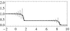
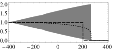
(b)  $t=10$	(e)

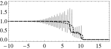
(c)  $t=50$

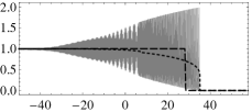
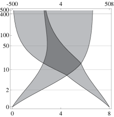
Figure 1: Plots (a)–(d) show the numerically computed solution of (1) and (e) the boundary of the one- (light gray) and two-phase (dark gray) regions computed using Whitham theory. The averaged solution, $\bar{u}$, is computed using Whitham averaging (cf. Levermore (1988)) and shown as dotted lines in (a)–(d); the solution of (2) is shown as dashed lines in (a)–(d). In all plots, $\varepsilon^{2}=0.001$, $h_{0}=1$, $h_{1}=0.4$, $h_{2}=0$ and $L=8$. The vertical axis in (e) is log-time and the horizontal axis is $-t\leq x\leq t+8$ (and matches the domain in (a)–(d)).

In Case I (     ), two one-phase DSWs form and propagate to the right (see Fig. 1a). When the shock front of the left DSW reaches the expanding oscillatory tail of the right DSW, they interact and form a quasi-periodic two-phase solution (see Fig. 1b). The shock front of the left DSW subsequently overtakes the shock front of the right DSW and forms a one-phase solution to the right of the two-phase region (see Fig. 1c). To the left of the two-phase solution, an essentially one-phase DSW tail emerges (see Fig. 1c); although the tail is weakly modulated by a quasi-periodic wave, its behavior is essentially one-phase. For large time, the two-phase region closes and a one-phase DSW remains (see Fig. 1d–e); Whitham theory indicates that the amplitude of the two-phase modulations decrease with time and result in an effectively one-phase DSW. This closing of the two phase region is suggested by the rigorous (Whitham theory) results in Grava and Tian (2002), though the authors studied smooth initial data. The computation of the boundaries of the one- and two-phase regions using multiphase Whitham theory are discussed later in this letter.

Although the (initial) shock front speed is different for DSWs and VSWs ($2h_{0}/3$ and $h_{0}/2$, respectively), the averaged DSWs are similar in behavior to VSWs (see Fig. 1a–d); in both, two shock waves merge to form a single shock wave.

(a)  $t=2$	(c)  $t=100$
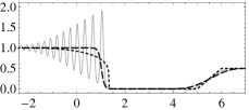
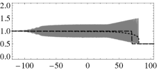
(b)  $t=10$	(d)  $t=800$

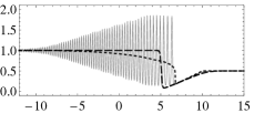
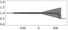
Figure 2: Plots of the numerical and averaged Whitham solutions of (1) for Case II (     ) where $\varepsilon^{2}=0.001$, $h_{0}=1$, $h_{1}=0$, $h_{2}=0.5$ and $L=5$.

For Case II (     ), a large DSW forms on the left and a small RW forms on the right (see Fig. 2a). The front of the DSW then interacts with the trailing edge of the RW; the interaction decreases the DSW’s speed and height (see Fig. 2b). The front of the DSW is faster than the front of the RW and overtakes it (see Fig. 2c). The size of the interaction region continues to expand with a DSW emerging in front with a small amplitude wave train behind, whose amplitude is proportional to $t^{-1/2}$ (see Fig. 2d). As in Case I (     ), the averaged DSW and the VSW (see Fig. 2) both tend to a single DSW (VSW) once the front of the DSW (VSW) passes the front of the RW.

Figure 3: The initial data regularization of Case II (     ) for $h_{0}>1$, $h_{1}=0$ and $h_{2}=1$; the dashed line is the initial condition, $u_{0}(x)$, and the solid lines are $r_{1}$, $r_{2}$, and $r_{3}$. The figure also gives the speed of the front and back of the DSW and RW at $t=0$.

We can use the one-phase Whitham equations to characterize the interaction of the DSW and RW in Case II (     ). In this context, Whitham theory consists of looking for a fully nonlinear single- or multi-phase solution whose parameters (amplitude, wave number and frequency) are slowing varying with respect to the phase(s) and then deriving new equations for the evolution of the slowly varying wave properties. The one-phase Whitham equations for (1) are

$$\frac{\partial r_{i}}{\partial t}+v_{i}(r_{1},r_{2},r_{3})\frac{\partial r_{i}}{\partial x}=0,\qquad i=1,2,3,$$ (4a)

where

$$v_{1} =V-\frac{2}{3}(r_{2}-r_{1})\frac{K(m)}{K(m)-E(m)},$$ (4b)

$$v_{2} =V-\frac{2}{3}(r_{2}-r_{1})\frac{(1-m)K(m)}{E(m)-(1-m)K(m)},$$

$$v_{3} =V+\frac{2}{3}(r_{3}-r_{1})\frac{(1-m)K(m)}{E(m)},$$

$V=(r_{1}+r_{2}+r_{3})/3$, $m=(r_{2}-r_{1})/(r_{3}-r_{1}),$ $K(m)$ is the complete elliptic integral of the first kind, and $E(m)$ is the complete elliptic integral of the second kind Gurevich and Pitaevskii (1974). Then, the asymptotic solution is

$$u_{a}(x,t)\approx r_{1}+r_{2}-r_{3}+2(r_{3}-r_{1})\operatorname{dn}^{2}\left(\theta;m\right),$$

where $\theta_{x}=\kappa$, $\theta_{t}=-\omega=-\kappa V$, $\kappa=\sqrt{(r_{3}-r_{1})/(6\varepsilon^{2})}$, and $r_{i}$ are slowly varying functions of $x$ and $t$. We can make a global dispersive regularization for the initial value problem (1) and (3) by choosing appropriate initial data for the $r_{i}$ Hoefer et al. (2006); Kodama (1999) which result in a global solution. A global dispersive regularization of Case II (     ) is shown in Fig. 3; the $r_{i}$ are taken to be nondecreasing, $r_{i}(x,0)<r_{i+1}(x,0)$ and $\bar{u}_{a}(x,0)=u(x,0)$ for all $x\in\mathbb{R}$.

(a)  $t=50$	(b)  $t=50$

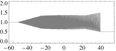
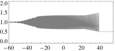
Figure 4: Plot (a) shows the Whitham approximation and (b) direct numerics of the solution of (1) for Case II (     ) with the same initial condition as Fig. 2.

In order to study the interaction we evolve the $r_{i}$ numerically. A simple and effective method for evolving the $r_{i}$ is to discretize the initial data regularization along the dependent variable, $r_{i}$, and then compute the shift in $x$ of each data point using (4). Fig. 4 compares a numerically evolved Whitham approximation with direct numerics for Case II (     ); the first order Whitham approximation does not capture the small quasi-periodic modulations in the tail because they are higher order effects. Both direct numerics and the Whitham approximation agree and show that for large enough time, the amplitude of the tail in Cases II (     ) is proportional to $t^{-1/2}$; this is typical of a uniform linear wave train when the total energy remains constant (cf. Whitham (1965)) and was observed in the context of a depression initial condition in El and Grimshaw (2002).

Multiphase Whitham theory is more complicated than one-phase Whitham theory and dates back to 1970 Ablowitz and Benny (1970); multiphase Whitham equations were developed for the KdV equation in Flaschka et al. (1980). The interaction of two DSWs from certain step-like data was recently analyzed in Hoefer and Ablowitz (2007) for the nonlinear Schrödinger equation. The one- and two-phase regions and the averaged solution in Case I (     ) are found by numerically evolving the two-phase Whitham equations for the KdV (see Levermore (1988)),

$$\frac{\partial r_{i}}{\partial t}+v_{i}(r_{1},\dotsc,r_{5})\frac{\partial r_{i}}{\partial x}=0,\qquad i=1,2,\dotsc,5,$$ (5)

where $v_{i}=(2r_{i}^{3}-\chi r_{i}^{2}-\beta_{1}r_{i}-\beta_{2})/(r_{i}^{2}-\alpha_{1}r_{i}-\alpha_{2}),$ $\chi=\sum_{j=1}^{5}r_{j}$, and $\alpha_{1}$, $\alpha_{2}$, $\beta_{1}$ and $\beta_{2}$ are solutions of

$$\begin{bmatrix}I_{1}^{1}&I_{1}^{0}\\ I_{2}^{1}&I_{2}^{0}\end{bmatrix}\begin{bmatrix}\alpha_{1}\\ \alpha_{2}\end{bmatrix}=\begin{bmatrix}I_{1}^{2}\\ I_{2}^{2}\end{bmatrix},\quad\begin{bmatrix}I_{1}^{1}&I_{1}^{0}\\ I_{2}^{1}&I_{2}^{0}\end{bmatrix}\begin{bmatrix}\beta_{1}\\ \beta_{2}\end{bmatrix}=\begin{bmatrix}2I_{1}^{3}-\chi I_{1}^{2}\\ 2I_{2}^{3}-\chi I_{2}^{2}\end{bmatrix},$$

with

$$I_{j}^{k}=\int_{r_{2j-1}}^{r_{2j}}\frac{\xi^{k}}{\sqrt{\prod_{i=1}^{5}(\xi-r_{i})}}\,d\xi.$$ (6)

(a)  $t=2$	(c)  $t=2$
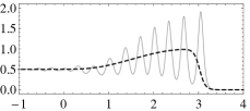
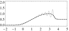
(b)  $t=50$	(d)  $t=50$

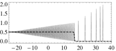
Figure 5: Plots of Cases (a) & (b) III (     ) with $h_{0}=0.5$, $h_{1}=1$, $h_{2}=0$ and (c) & (d) V (     ) with $h_{0}=0$, $h_{1}=1$, $h_{2}=0.5$, where $\varepsilon^{2}=0.001$ and $L=2$. There are six solitons in both cases, see (8).

In Case III (     ), a small RW forms on the left and a large DSW forms on the right. The front of the RW then interacts with the tail of the DSW and reduces the amplitude of the waves—essentially cutting off the top of the box. Since the front speed of the RW is less than the front speed of the initial DSW, a finite number of solitons can escape the interaction (see Fig. 5). These solitons have no analogue in the VSW solution of Case III (     ). We can compute the number of solitons which escape using IST theory.

From IST theory, the number of solitons correspond to the time-independent number of zeroes of $a(k)$ (which is the number of poles of the reflection coefficient $R\equiv b(k)/a(k)$) in the upper half $k$-plane. Associated with (1), the data $a(k)$ is defined by

$$\phi(x;k) \equiv a(k)\bar{\psi}(x;k)+b(k)\psi(x;k),$$

$$\bar{\phi}(x;k) \equiv\bar{a}(k)\psi(x;k)+\bar{b}(k)\bar{\psi}(x;k),$$

corresponding to the eigenfunctions,

$$\phi(x;k)\sim e^{-ik_{0}x},\qquad\bar{\phi}(x;k)\sim e^{ik_{0}x},\qquad\text{as }x\to-\infty,$$

$$\psi(x;k)\sim e^{ik_{2}x},\qquad\bar{\psi}(x;k)\sim e^{-ik_{2}x},\qquad\text{as }x\to+\infty,$$

which satisfy the Schrödinger scattering problem,

$$w_{xx}+w\{u/6+k^{2}\}/\varepsilon^{2}=0.$$ (7)

The solution of (7), at $t=0$, is

$$w(x)=\begin{cases}Ae^{ik_{0}x}+Be^{-ik_{0}x},&x<0,\\ Ce^{ik_{1}x}+De^{-ik_{1}x},&0<x<L,\\ Ee^{ik_{2}x}+Fe^{-ik_{2}x},&x>L,\end{cases}$$

where $k_{0}=\sqrt{h_{0}/6+k^{2}}/\varepsilon$, $k_{1}=\sqrt{h_{1}/6+k^{2}}/\varepsilon$, and $k_{2}=\sqrt{h_{2}/6+k^{2}}/\varepsilon$. The eigenfunctions, $\phi$, $\bar{\phi}$, $\psi$ and $\bar{\psi}$ are determined by requiring that $w$ and $w^{\prime}$ are continuous across $x=0$ and $x=L$. Indeed, $\phi$ is found by taking $A=0$ and $B=1$ and then solving for $C$, $D$, $E\equiv b(k)$, $F\equiv a(k)$, so that

$$a(k)=e^{ik_{2}L}\frac{k_{0}+k_{2}}{2k_{2}}\bigg{\{}\cos(k_{1}L)-i\frac{k_{1}^{2}+k_{0}k_{2}}{k_{1}(k_{0}+k_{2})}\sin(k_{1}L)\bigg{\}}.$$

Since $e^{ik_{2}L}(k_{0}+k_{2})/(2k_{2})\neq 0,$ the zeroes of $a(k)$ occur when $\tan(k_{1}L)=ik_{1}(k_{0}+k_{2})/(k_{1}^{2}+k_{0}k_{2})$.

It can be shown that the zeroes of $a(k)$ are purely imaginary; thus, we let $k=i\kappa$ (where $\kappa\in\mathbb{R}$ and $\kappa>0$). For Case III (     ), where $h_{1}=1>h_{0}=h_{*}$ and $h_{2}=0$, the zeroes of $a(i\kappa)$ occur when

$$\tan\left(\sqrt{1/6-\kappa^{2}}L/\varepsilon\right)=\frac{\sqrt{1/6-\kappa^{2}}\left(\sqrt{\kappa^{2}-h_{*}/6}+\kappa\right)}{1/6-\kappa^{2}-\kappa\sqrt{\kappa^{2}-h_{*}/6}}.$$ (8)

The number of periods for $\sqrt{h_{*}/6}\leq\kappa\leq\sqrt{1/6}$ of the RHS of (8), $L\sqrt{1-h_{*}}/(\varepsilon\pi\sqrt{6})$, is an estimate of the number of solitons. The number of zeroes determined using (8) exactly corresponds to the number of solitons observed using direct numerics (for various values of $h_{*}$, $L$ and $\varepsilon$)!

(a)  $t=5$	(b)  $t=400$

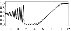
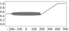
Figure 6: Plots of the solution of (1) for Case IV (     ) where $\varepsilon^{2}=0.001$, $h_{0}=0.5$, $h_{1}=0$, $h_{2}=1$ and $L=5$.

In Case IV (     ), a small DSW forms on the left and a large RW forms on the right (see Fig. 6a). As in Case II (     ), the front of the DSW interacts with the trailing edge of the RW and decreases the DSW’s amplitude and speed. Unlike Case II (     ), the front of the DSW does not overtake the front of the RW. The DSW becomes a small amplitude tail on the left of the RW and decreases in amplitude proportional to $t^{-1/2}$ (see Fig. 6b).

As in Case III (     ), Case V (     ) cannot be completely characterized using Whitham averaging. For Case V (     ), a large RW forms on the left and a small DSW forms on the right; the front of the RW interacts with the tail of the DSW and results in a RW and a finite number of solitons. The number of solitons corresponds to the number of zeroes of (8) where where $h_{0}=0$ and $h_{1}=1>h_{2}=h_{*}$.

In Case VI (     ), two rarefaction waves form; the small amplitude oscillatory tail (see for instance the RW in 6a) of the right RW interacts with the front of left RW; the tail of the right and left RW then interact to form a small amplitude, modulated, quasi-periodic tail; this modulation decreases with time and Case VI (     ) tends to a pure RW for large time.

We numerically solve (1) and (2) using an adaptation of the modified exponential time-differencing fourth-order Runge-Kutta (ETDRK4) method (see Kassam and Trefethen (2005)). We use this (sophisticated) numerical method because (1) is very stiff and standard numerical methods require the time step to be $O(\varepsilon^{3})$, while for ETDRK4 the time step need only be $O(\varepsilon)$. When this numerical scheme was used to compute a known exact solution, it was accurate to more than six decimal digits.

For spectral accuracy when using the ETDRK4 method, the initial data must be both smooth and periodic. Therefore, we differentiate (1) with respect to $x$ and define $v\equiv u_{x}$ to get $v_{t}+(uv)_{x}+\varepsilon^{2}v_{xxx}=0.$ Transforming to Fourier space gives $\hat{v}_{t}=i\varepsilon^{2}k^{3}\hat{v}-ik\widehat{uv}\equiv\mathbf{L}\hat{v}+\mathbf{N}(\hat{v},t),$ where we define $(\mathbf{L}\hat{v})(k)\equiv i\varepsilon^{2}k^{3}\hat{v}$ and $\mathbf{N}(\hat{v},t)=\mathbf{N}(\hat{v})\equiv-ik\mathcal{F}\{[h_{0}+\int_{-\infty}^{x}\mathcal{F}^{-1}(\hat{v})dx^{\prime}]\mathcal{F}^{-1}(\hat{v})\}$. It is important that the integral in $\mathbf{N}$ is computed using a spectrally accurate method. Moreover, we approximate the initial step data with the analytic function $2wv(x,0)=(h_{2}-h_{1})\operatorname{sech}^{2}[(x-L)/w]+(h_{1}-h_{0})\operatorname{sech}^{2}(x/w)$, where $w$ is small. See Kassam and Trefethen (2005) for details about how this $\mathbf{L}$ and $\mathbf{N}$ are used to numerically compute the solution of (1).

For large time Case I (     ) and II (     ) go to a single DSW, while Case IV (     ) and VI (     ) go to a single RW; this is consistent with VSW theory. However, unlike VSW theory, Case III (     ) and V (     ) form a finite number of solitons in addition to the DSW or RW, respectively. Moreover, unlike VSW theory, Case I (     ) exhibits a transient two-phase region and Case II (     ) and IV (     ) have a small amplitude tail which decays at a rate proportional to $t^{-1/2}$.