Quasi-Optical Characterization of Dielectric and Ferrite Materials

17th International Symposium on Space THz Technology, Paris 2006 May 10-12

I Introduction

In the millimeter-submillimeter range, Quasi-Optical (QO) benches can be relatively compact, typically of order 10cm wide and 1m long. The focussing elements used in these benches are dielectric lenses, or off-axis elliptical mirrors. Simultaneous Transmission $T$ (corresponding to the complex $S21$ parameter), and Reflection $R$ (corresponding to the complex S ii parameter) are vectorially detected versus frequency in the frequency range 40-700 GHz. A parallel-faced slab, thickness $e$, of dielectric material is placed at a Gaussian beam waist within the system. It is straightforward to determine the refractive index $n$ (with $\varepsilon^{\prime}=n^{2}$) of this sample from the phase rotation $\Delta\Phi$:

$$(n-1)e/\lambda=\Delta\Phi/360$$ (1)

The loss factor $\tan\delta$ is known from the damping of the transmitted signal, Fig. 1:

$$\tan\delta=1.1~{}\alpha\textrm{(dB/cm)}/nF\textrm{(GHz)}$$ (2)

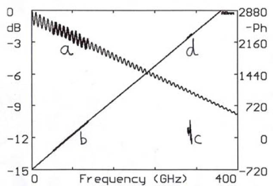
Figure 1: Transmission through 10.95 mm nylon. (a) thick line is the observed amplitude in V-W bands. (b) is the corresponding phase (represented in opposite sense for clarity). Around 305 GHz, the measured (d) phase value, in good alignment with extrapolated (b), shows that the permittivity $\varepsilon^{\prime}=3.037$ is constant with frequency. On the contrary, the position of the amplitude (c) shows that the loss, which was $\tan\delta=0.013$ at low frequencies, has increased to $\tan\delta=0.019$, since (c) is far from the extrapolated (a).

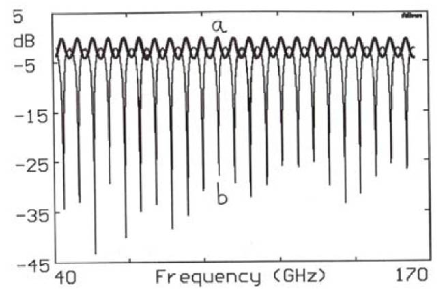
Figure 2: Transmission (a) and reflection (b) through 9.53 mm AIN. The dielectric parameters, observed in V-W-D bands, are constant with $\varepsilon^{\prime}=8.47S$, $\tan\delta=0.0007$, also measured the same in cavity at 140.4 GHz.

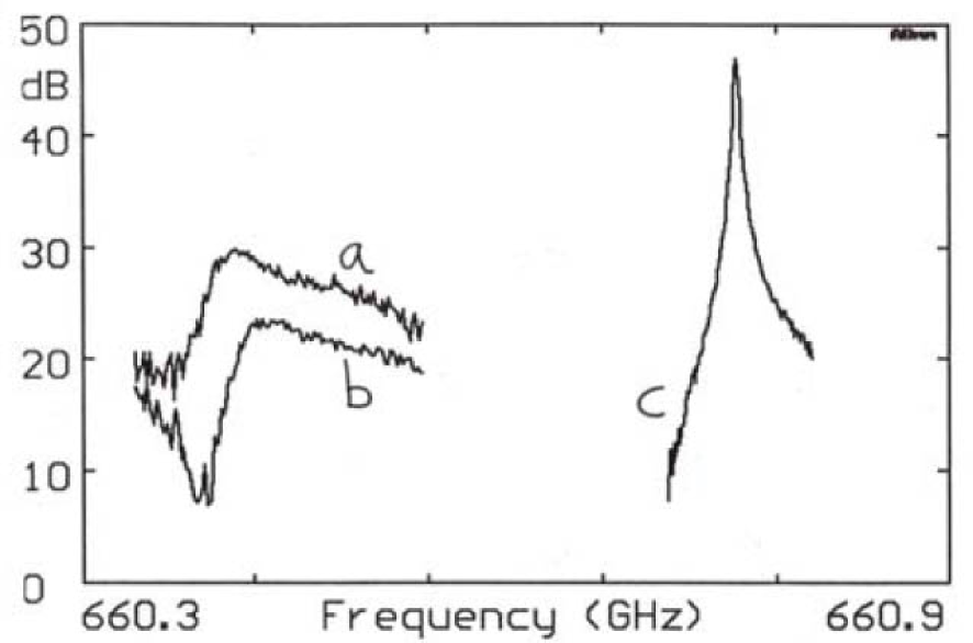
Figure 3: Resonances observed in an open Fabry-Perot cavity loaded by a 10.03 mm thick slab of slightly birefringent Teflon. In (a) the RF field is along the large index axis $\varepsilon^{\prime}=2.0664$, in (b) along the small index axis $\varepsilon^{\prime}=2.0636$. In (c), is the empty cavity resonance. The $\varepsilon^{\prime}$ anisotropy is exactly the same as observed at 135 GHz. The loss has increased from $\tan\delta=0.0003$ at 135 GHz to $0.0008$ at 660 GHz.

The samples in this measurement system act as Fabry-Perot resonators with maximum transmission corresponding to minimum reflection, and vice-versa (see Fig.2), with a period $\Delta F=c/(2ne)$. For very low loss materials, there is however some difficulty in measuring the loss term by a single crossing, since the maximum transmission is very close to 0 dB. One uses the cavity perturbation technique, which makes visible the low losses after many crossings through the dielectric slab (see Fig.3).

II Experimental Setup for free-space propagation

In V-W-D bands (extended down to ca 41 GHz, close to the V-band cutoff), we use the following waveguide components. On the source side, the harmonic Generator HG sends its millimeter power through a full-band Faraday isolator FI1, cascaded with a fixed attenuator AT1, a directional coupler DC (from port 2 to port 1) and a Scalar Horn SH1. The reflection (Channel 1) is detected by a Harmonie Mixer HM1 attached to output 3 of the DC through the isolator F12. On the transmission detection side, the Scalar Horn SH2 sends the collected wave to the Harmonic Mixer HM2 (Channel 2) through cascaded AT2 and FI3.

III Isolators FIs and Attenuators ATs, what for?

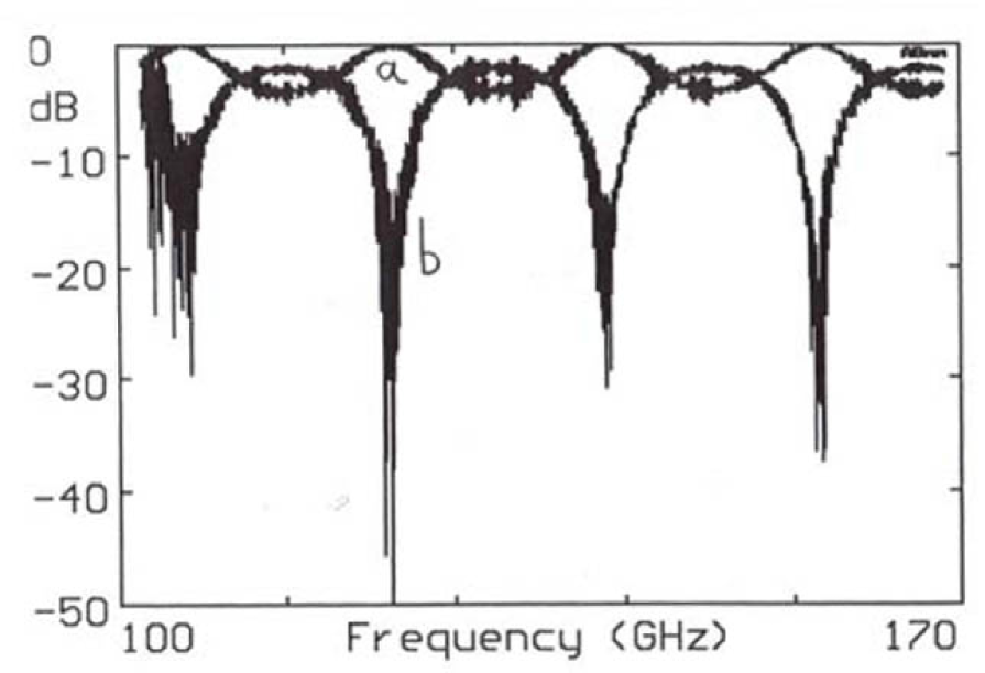
Figure 4: Transmission (a) and reflection (b) through a 3 mm thick $MgAl_{2}O_{3}$ slab. These raw data show parasitic standing waves appearing as noise

The first use of isolators is to assume a one-way propagation. The non-linear devices HG and HMs contain Schottly diodes. In case the wave can travel go-and-back from one device to the other, the combination of non-linear and standing waves effect can send microwave power from a given harmonic to another harmonic [1] . This is why multipliers cascaded without isolation (like $\times 2~{}\times 3$ ) can create unexpected harmonics (like $\times 5~{}\times 7$). We have also observed, for instance with cascaded tripiers ($\times 3~{}\times 3$ ), measurable amounts of unexpected $\times 10,~{}\times 11$, or $\times 12$ [2]. The devices HG and HMs can be viewed as Schottky diodes across waveguides, meaning unmatched structures. The second use of the FIs is to reduced the VSWR. Their typical return is -20 dB (VSWR ca 1.22). We improve this value down to - 30 dB (VSWR ca 1.07) when introducing the fixed attenuators ATs.

IV Experimental difficulties

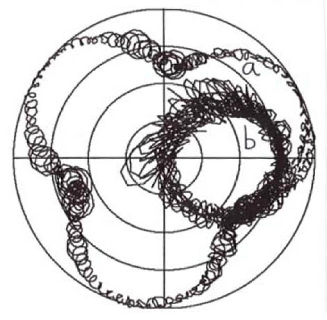
Figure 5: Polar plot of Fig.5

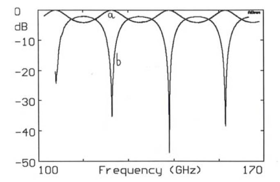
Figure 6: Same as Fig.4 after FT filtering.. The measured dielectric parameters are $\varepsilon^{\prime}=8.080$, and $\tan\delta=0.0005$.

Figure 7: Polar plot of Fig.6

Figure 8: Transmission across 9.97 mm sapphire, from 469 GHz, point (a), to 479 GHz, point (b), with absorbers, total 30 dB, between source and detection, in order to reduce the parasitic standing waves. Despite this strong attenuation, the measurement quality is far from being as good as at lower frequencies, like in Fig.7. In (c) is the 473.3 to 474.5 GHz sweep without absorbers, showing big standing waves effects.

Even with our best benches using the complete chains assuming a low VSWR ( $<1.1$ see sec III), the parasitic standing waves effects are clearly visible on raw data, Fig.4-5. They are due to multiple reflections between the sample, placed perpendicular to the beam, and the components of the bench. However, they can be completely filtered by FT calculations (see Figs.6-7). There is a lack of FIs waveguide isolators above 220 GHz and, as far as we know, of DCs above 400 GHz. As a consequence, characterization at submillimeter wavelengths is operated by transmission only, and is much more difficult, Fig.8, than in V-W-D-bands, due to large parasitic standing waves.

V Non-magnetized ferrites characterization

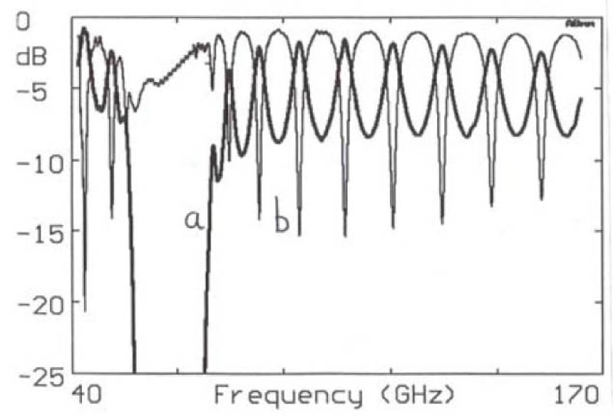
Figure 9: Transmission (a), and reflection (b) through a 2.55 mm thick non-magnetized TDK ferrite sample.

In the case of ferrite materials, the properties are very strongly frequency dependent. Non-magnetized ferrites show a strong resonance in the range 50-60 GHz (see Fig.9), and the asymptotic behavior, far from resonance, starts to be visible beyond 200 GHz. Measurements performed at 475 GHz on six samples give $\varepsilon^{\prime}$ in the range 18.8 to 21.4, and $\tan\delta$ in the range 0.012 to 0.018.

VI Magnetized ferrites

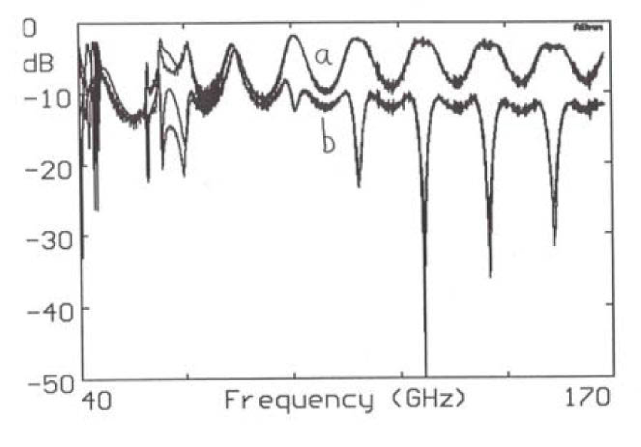
Figure 10: Transmission through 2 mm magnetized sample FB6H1, (a) is $-45^{\circ}$, (b) is $+45^{\circ}$. Experimental traces and superimposed fittings.

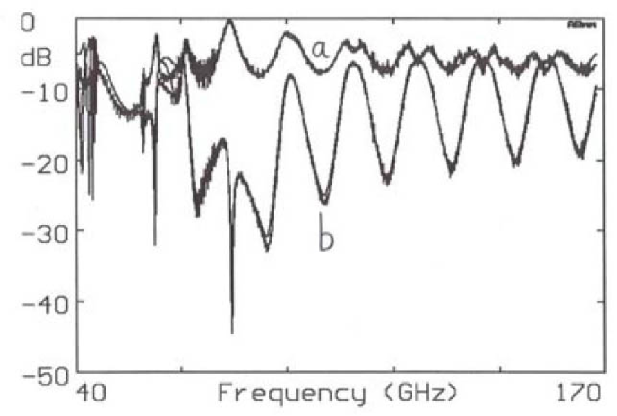
Figure 11: Same as Fig.10, where (a) is $90^{\circ}$ and (b) is $0^{\circ}$.

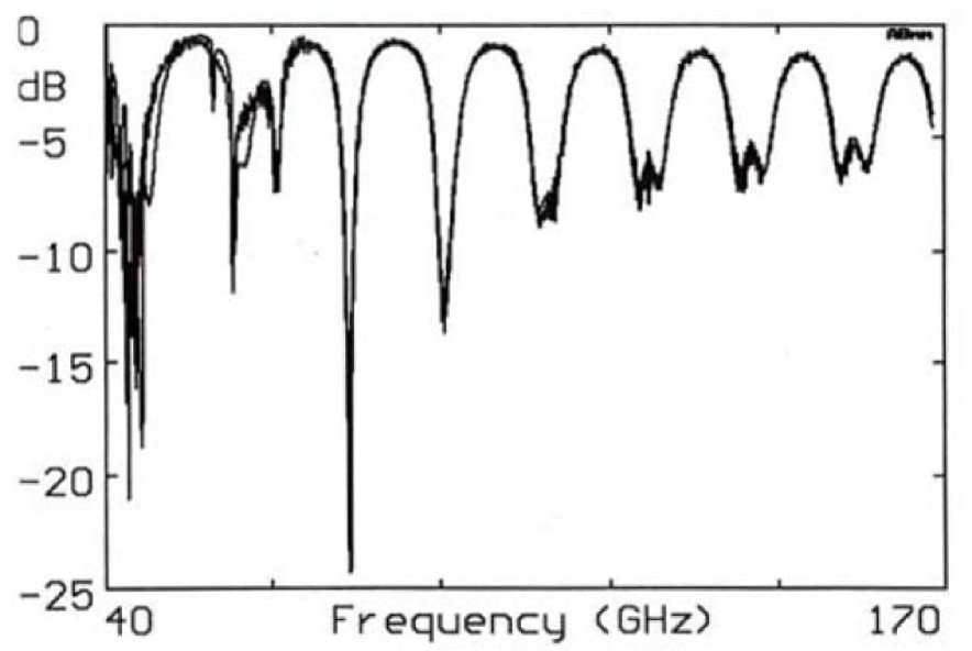
Figure 12: Reflection at $0^{\circ}$ from the magnetized sample FB6H1, experiment and fit.

When a ferrite is submitted to an external, or internal, magnetic field, there is a strong anisotropy of propagation according to the circular polarization of the crossing electromagnetic wave [3]. The two refractive indices $n^{\pm}$ are given by:

$$(n^{\pm})^{2}=\varepsilon^{\prime}[1+F_{m}/(F_{0}\pm F)]$$

, where $F$ is the frequency, $F_{0}$ the Larmor frequency, $F_{m}$ is proportional to the remanent magnetization of the ferrite, and $\varepsilon^{\prime}$ is the dielectric constant. Any linearly polarized wave, like ours at the SH outputs, can be viewed as the superposition of two opposite senses circularly polarized components. After crossing the ferrite, one of the components has experienced a larger retardation than the other, so that, when recombining the two, the plane of linear polarization has been rotated. In order to characterize magnetized ferrite samples, it is necessary to measure not only the transmitted signals with a polarization parallel to the source, but also those with polarization at $\pm 45$ degrees, and 90 degrees, see Figs.10-11-12.

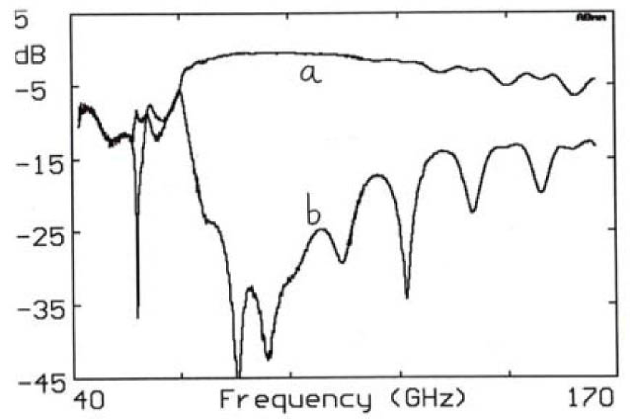
Figure 13: Reflection at $0^{\circ}$ from the magnetized sample FB6H1, experiment and fit.

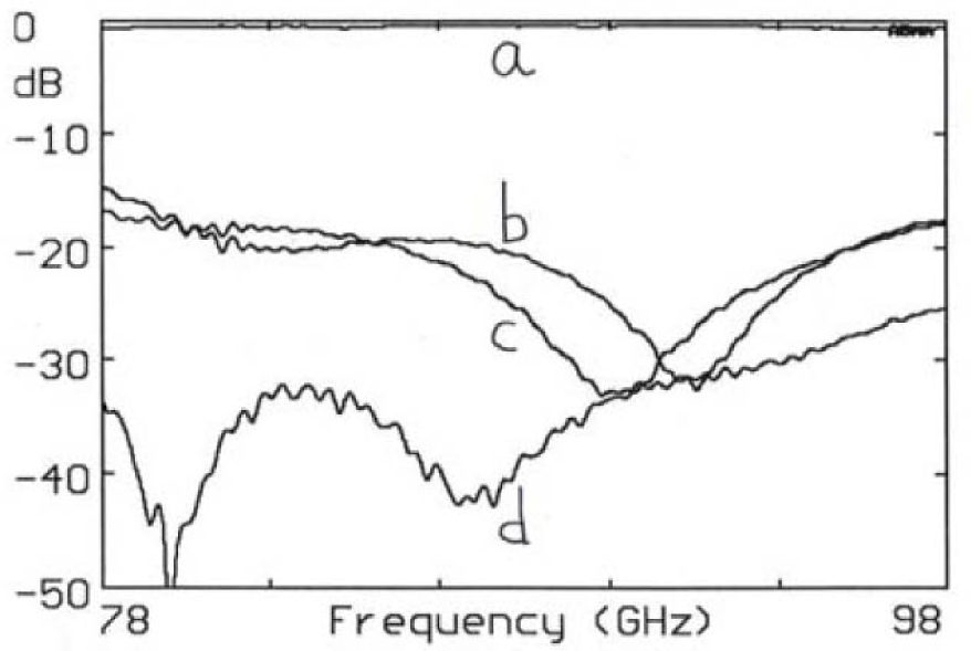
Figure 14: Reflection at $0^{\circ}$ from the magnetized sample FB6H1, experiment and fit.

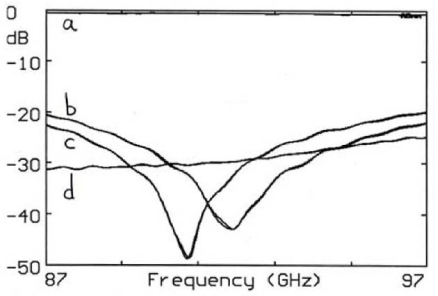
Figure 15: Reflection at $0^{\circ}$ from the magnetized sample FB6H1, experiment and fit.

When adding an anti-reflection coating on each side of the magnetized ferrite, the thickness of the ferrite being chosen so that the rotation through it is $45^{\circ}$ at the required frequency, one can obtain a good QO Faraday Rotator, Fig.13. The performances observed around the central frequency, Figs.14-15, are at least similar (for isolation or matching) or better (for insertion loss) than the equivalent waveguide isolators.

VII QOFRs expected to become submillimeter isolators and directional Couplers

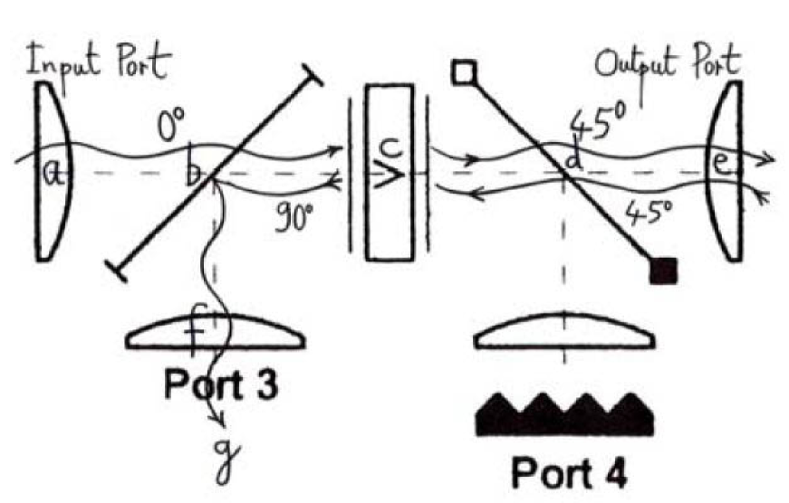
Figure 16: Schematic diagram of a QOFR used as an isolator (there is a inatched load at (g) ) Port 3, or as a Directional Coupler DC for detecting reflected waves at (g). The vertical polarisation at (a), fully transmitted through the horizontal grid (b), rotates by $+45^{\circ}$ through the magnetized ferrite (c), then is fully transmitted through the $-45^{\circ}$ grid (d). Any reflected signal without polarisation change will cross back (d) without loss, then will rotate by $+45^{\circ}$ again across (c), becoming horizontal, then will be totally reflected by the horizontal grid (b), towards Port 3.

Our QO benches studying samples perpendicular to the wave beam, are, up to now, less performing in submillimeter (Fig.8) than in the millimeter domain (Fig.7), due to parasitic standing waves. Introducing the appropriate QO Faraday Rotators will reduce this effect. On figure 16 one can see how a QOFR can be simply configurated for that purpose.

VIII Conclusion

Precise and quick QO measurements in the 40-170 GHz interval, in particular for ferrites characterization, opens the possibility of similar precise and easy measurements at high frequencies, including the submillimeter domain, by using these ferrites in QOFRs in progress [4]. At the same time, widely sweepable solid-state submillimeter sources must be developed.

References

- [1] P. Goy, M. Gross, and S. Caroopen. Millimeter and Submillimeter Wave Vector Measurements with a network analyzer up to 1000 GHz. Basic Principles and Applications. In 4th International Conference on Millimeter and Submillimeter Waves and Applications, San Diego, California USA, 1998 Jul 20-23.
- [2] P. Goy. Private communicatuions. 2005-2006.
- [3] R.I. Hunter, D.A. Robertson, and G.M. Smith. Ferrite Materials for Quasi-Optical Devices and Applications. In Int Confon IR and mmWaves, Karlsruhe, 2004 Sep 27 - Oct 1.
- [4] P. Goy R.I. Hunter, D.A. Robertson and G.M. Smith. Characterization of Ferrite Materials for use in Quasi-Optical Faraday Rotators. In to be published.