Schnyder woods for higher genus triangulated surfaces, with applications to encoding

Abstract.

Schnyder woods are a well-known combinatorial structure for plane triangulations, which yields a decomposition into 3 spanning trees. We extend here definitions and algorithms for Schnyder woods to closed orientable surfaces of arbitrary genus. In particular, we describe a method to traverse a triangulation of genus $g$ and compute a so-called $g$-Schnyder wood on the way. As an application, we give a procedure to encode a triangulation of genus $g$ and $n$ vertices in $4n+O(g\log(n))$ bits. This matches the worst-case encoding rate of Edgebreaker in positive genus. All the algorithms presented here have execution time $O((n+g)g)$, hence are linear when the genus is fixed.

This is the extended and revised journal version of a conference paper with the title “Schnyder woods generalized to higher genus triangulated surfaces”, which appeared in the Proceedings of the ACM Symposium on Computational Geometry 2008 (pages 311-319).

1. Introduction

Schnyder woods are a nice and deep combinatorial structure to finely capture the notion of planarity of a graph. They are named after W. Schnyder, who introduced these structures under the name of realizers and derived as main applications a new planarity criterion in terms of poset dimensions [37], as well as a very elegant and simple straight-line drawing algorithm [38]. There are several equivalent formulations of Schnyder woods, either in terms of angle labeling (Schnyder labeling) or edge coloring and orientation or in terms of orientations with prescribed out-degrees. The most classical formulation is for the family of maximal plane graphs, i.e., plane triangulations, yielding the following striking property: the internal edges of a triangulation can be partitioned into three trees that span all inner vertices and are rooted respectively at each of the three vertices incident to the outer face. Schnyder woods, and more generally $\alpha$-orientations, received a great deal of attention [38, 19, 25, 21]. From the combinatorial point of view, the set of Schnyder woods of a fixed triangulation has an interesting lattice structure [7, 3, 20, 15, 16], and the nice characterization in terms of spanning trees motivated a large number of applications in several domains such as graph drawing [38, 25], graph coding and random sampling [14, 24, 4, 33, 22, 5, 10, 1]. Previous work focused mainly on the application and extension of the combinatorial properties of Schnyder woods to 3-connected plane graphs [19, 25]. In this article, we focus on triangulations, but, which is new, we consider triangulations in arbitrary genus.

1.1. Related Work

1.1.1. Vertex spanning tree decompositions

In the area of tree decompositions of graphs there exist some works dealing with the higher genus case. We mention one recent attempt to generalize Schnyder woods to the case of toroidal graphs [6] (genus $1$ surfaces), based on a special planarization procedure. In the genus $1$ case it is actually possible to choose two adjacent non-contractible cycles, defining a so-called tambourine, whose removal makes the graph planar; the graph obtained can thus be endowed with a Schnyder wood. In the triangular case this approach yields a process for computing a partition of the edges into three edge-disjoint spanning trees plus at most $3$ edges. Unfortunately, as pointed out by the authors, the local conditions of Schnyder woods are possibly not satisfied for a large number of vertices, because the size of the tambourine might be arbitrary large. Moreover, it is not clear how to generalize the method to genus $g\geq 2$.

1.1.2. Planarizing graphs on surfaces

A possible solution to deal with Schnyder woods (designed originally for plane triangulations) in higher genus would consist in performing a planarization of the surface. Actually, given a triangulation $\mathcal{T}$ with $n$ vertices on a surface $\mathcal{S}$ of genus $g$, one can compute a cut-graph or a collection of $2g$ non-trivial cycles, whose removal makes $\mathcal{S}$ a topological disk (possibly with boundaries). There is a number of recent contributions [8, 17, 18, 27, 28, 43] for the efficient computation of cut-graphs, optimal (canonical) polygonal schemas and shortest non-trivial cycles. For example some work makes it possible to compute polygonal schemas in time $O(gn)$ for a triangulated orientable manifold [28, 43]. Nevertheless we point out that a planarization approach would not be best suited for our purpose. From the combinatorial point of view this would imply to deal with boundaries of arbitrary size (arising from the planarization procedure), as non-trivial cycles can be of size $\Omega(\sqrt{n})$, and cut-graphs have size $O(gn)$. Moreover, from the algorithmic complexity point of view, the most efficient procedures for computing small non-trivial cycles [8, 27] require more than linear time, the best known bound being currently of $O(n\log n)$ time.

1.1.3. Schnyder trees and graph encoding

One of our main motivations for generalizing Schnyder woods to higher genus is the great number of possible applications in graph encoding and mesh compression that take advantage of spanning tree decompositions [26, 34, 41], and in particular of the ones underlying Schnyder woods (and related extensions) for planar graphs [1, 13, 14, 22, 24, 33]. The combinatorial properties of Schnyder woods and the related characterizations (canonical orderings [25]) for planar graphs yield efficient procedures for encoding tree structures based on multiple parenthesis words. In this context a number of methods have been proposed for the simple compression [24] or the succinct encoding [14, 13] of several classes of planar graphs. More recently, this approach based on spanning tree decompositions has been further extended to design a new succinct encoding of labeled planar graphs [1]. Once again, the main ingredient is the definition of three traversal orders on the vertices of a triangulation, directly based on the properties of Schnyder woods. Finally we point out that the existence of minimal orientations (orientations without counterclockwise directed cycles) recently made it possible to design the first optimal (linear time) encoding for triangulations and $3$-connected plane graphs [22, 33], based on bijective correspondences with families of plane trees. Such bijective constructions, originally introduced by Schaeffer [36], have been applied to many families of plane graphs (also called planar maps) and give combinatorial interpretations of enumerative formulas originally found by Tutte [42]. In recent work, some of these bijections are extended to higher genus [12, 11], but a bijective construction for triangulations or 3-connected plane graphs in higher genus is not yet known. The difficulty of extending combinatorial constructions to higher genus is due the fact that some fundamental properties, such as the Jordan curve theorem, hold only in the planar case (genus $0$). Nevertheless, the topological approach used by Edgebreaker (using at most $3.67$ bits per vertex in the planar case) has been successfully adapted to deal with triangulated surfaces having arbitrary topology: orientable manifolds with handles [31] and also multiple boundaries [29]. Using a different approach, based on a partitioning scheme and a multi-level hierarchical representation [9], it is also possible to encode a genus $g$ triangulation with $f$ faces and $n$ vertices using $2.175f+O(g\log f)+o(f)$ bits (or $4.35n+o(gn)$ bits) which is asymptotically optimal for surfaces with a boundary: nevertheless, the amount of additional bits hidden in the sub-linear $o(n)$ term can be quite large, of order $\Theta(\frac{n}{\log n}\log\log n)$.

1.2. Contributions

Our contributions start in Section 4, where we give a definition of Schnyder woods for triangulations of arbitrary genus, which extends the definition of Schnyder for plane triangulations. Then we describe a traversal algorithm to actually compute such a so-called $g$-Schnyder wood for any triangulation of genus $g$, in time $O((n+g)g)$. Again our procedure extends to any genus the known procedures to traverse a plane triangulation and compute a Schnyder wood on the way [37, 7]. Finally, in Section 5, we show that a $g$-Schnyder wood yields an algorithm to efficiently encode a triangulation of genus $g$ and with $n$ vertices, in $4n+O(g\log(n))$ bits. This is again an extension to arbitrary genus of a procedure described in [24, 2] to encode plane triangulations. Our result matches the same worst-case encoding rate as Edgebreaker [34], which uses at most $3.67n$ bits in the planar case, but requires up to $4n+O(g\log n)$ bits for meshes with positive genus [31, 29]. As far as we know this is the best known rate for linear time (in fixed genus) encoding of triangulations with positive genus $g$, quite close to the information theory bound of $3.24n+\Omega(g\log n)$ bits (a more detailed discussion is given in Section 5).

2. Schnyder woods for Plane Triangulations

2.1. Definition

A plane triangulation $\mathcal{T}$ is a graph with no loops nor multiple edges and embedded in the plane such that all faces have degree 3. The edges and vertices of $\mathcal{T}$ incident to the outer face are called the outer edges and outer vertices. The other ones are called the inner edges and inner vertices.

We recall here the definition of Schnyder woods for plane triangulations, which we will later generalize to higher genus. While the definition is given in terms of local conditions, the main structural property, as stated in Fact 1, is more global, namely a partition of the inner edges into 3 trees, see Figure 1 .

Definition 1 ([38]).

Let $\mathcal{T}$ be a plane triangulation, and denote by $v_{0},v_{1},v_{2}$ the outer vertices in counterclockwise (ccw) order around the outer face. A Schnyder wood of $\mathcal{T}$ is an orientation and labeling, with labels in $\{0,1,2\}$ of the inner edges of $\mathcal{T}$ so as to satisfy the following conditions:

• root-face condition: for $i\in\{0,1,2\}$, the inner edges incident to the outer vertex $v_{i}$ are all ingoing of color $i$.

• local condition for inner vertices: For each inner vertex $v$, the edges incident to $v$ in counterclockwise (ccw) order are: one outgoing edge colored $2$, zero or more incoming edges colored $1$, one outgoing edge colored $0$, zero or more incoming edges colored $2$, one outgoing edge colored $1$, and zero or more incoming edges colored $0$, which we write concisely as

  $$(\mathrm{Seq}(\mathrm{In}\ \!1),\mathrm{Out}\ \!0,\mathrm{Seq}(\mathrm{In}\ \!2),\mathrm{Out}\ \!1,\mathrm{Seq}(\mathrm{In}\ \!0),\mathrm{Out}\ \!2).$$

Fact 1 ([38]).

Each plane triangulation $\mathcal{T}$ admits a Schnyder wood. Given a Schnyder wood on $\mathcal{T}$, the three directed graphs $T_{0}$, $T_{1}$, $T_{2}$ induced by the edges of color $0$, $1$, $2$ are trees that span all inner vertices and are naturally rooted at $v_{0}$, $v_{1}$, and $v_{2}$, respectively.

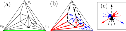
Figure 1. (a) A rooted planar triangulation, (b) endowed with a Schnyder wood. (c) The local condition of Schnyder woods.

2.2. Computation of Schnyder woods for plane triangulations

In this section we briefly review a well-known linear time algorithm designed for computing a Schnyder wood of a plane triangulation, following the presentation by Brehm [7]. It is convenient here (in view of the generalization to higher genus) to consider a plane triangulation as embedded on the sphere $S$, with a marked face that plays the role of the outer face. The procedure consists in growing a region $C$, called the conquered region, delimited by a simple cycle $B$ ($B$ is considered as part of $C$) . Initially $C$ consists of the root-face (as well as its incident edges and vertices). A chordal edge is defined as an edge not in $C$ but with its two extremities on $B$. A free vertex is a vertex of $B\setminus\{v_{0},v_{1}\}$ with no incident chordal edges. One defines the conquest of such a vertex $v$ as the operation of transferring to $C$ all faces incident to $v$, as well as the edges and vertices incident to these faces; the boundary $B$ of $C$ is easily verified to remain a simple cycle. Associated with a conquest is a simple rule to color and orient the edges incident to $v$ in the exterior region. Let $v_{r}$ be the right neighbor and $v_{l}$ the left neighbor of $v$ on $B$, looking toward $\mathcal{T}\backslash C$ (in the figures, toward the shaded area). Orient outward of $v$ the two edges $(v,v_{r})$ and $(v,v_{l})$; assign color $0$ to $(v,v_{r})$ and color $1$ to $(v,v_{l})$. Orient toward $v$ and color $2$ all edges exterior to $C$ incident to $v$ (these edges are between $(v,v_{r})$ and $(v,v_{l})$ in ccw order around $v$).

The algorithm for computing a Schnyder wood of a plane triangulation with $n$ vertices is a sequence of $n-2$ conquests of free vertices, together with the operations of coloring and orienting the incident edges (the initial conquest, always applied to the vertex $v_{2}$, is a bit special: the edges going to the right and left neighbors are not colored nor oriented, since these are outer edges).

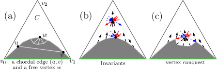
Figure 2. (a) A chordal edge and a free vertex, (b) the invariants valid in the planar case, (c) the result of a vertex conquest.

The correctness and termination of the traversal algorithm described above is based on the following fundamental property illustrated in Figure 3. A planar chord diagram (i.e., a topological disk with chordal edges that do not cross each other) with root-edge $\{v_{0},v_{1}\}$ always has on its boundary a vertex $v\notin\{v_{0},v_{1}\}$ not incident to any chord, see for instance [7] for a detailed proof.

Figure 3. In a planar chord-diagram with a root-edge $e=\{v_{0},v_{1}\}$, there must be a vertex $v$ not incident to $e$ nor to any chord.

One proves that the structure computed by the traversal algorithm is a Schnyder wood by considering some invariants (see Figure 2):

• the edges that are already colored and directed are the inner edges of $C\backslash B$.

• for each inner vertex $v$ of $C\backslash B$, all edges incident to $v$ are colored and directed in such a way that the Schnyder rule (Figure 1(c)) is satisfied;

• every inner vertex $v\in B$ has exactly one outgoing edge $e$ in $C\backslash B$; and this edge has color $2$. Let $v_{r}$ be the right neighbor and $v_{l}$ the left neighbor of $v$ on $B$, looking toward $\mathcal{T}\backslash C$. Then all edges strictly between $(v,v_{r})$ and $e$ in cw order around $v$ are ingoing of color $1$ and all edges strictly between $e$ and $(v,v_{l})$ in cw order around $v$ are ingoing of color $0$.

These invariants are easily checked to be satisfied all along the procedure (see [7] for a detailed presentation), which yields the following result:

Lemma 2 (Brehm [7]).

Given a planar triangulation $\mathcal{T}$ with outer face $(v_{0},v_{1},v_{2})$ the traversal algorithm described above computes a Schnyder wood of $\mathcal{T}$ and can be implemented to run in time $O(n)$.

Note that a triangulation $\mathcal{T}$ can have many different Schnyder woods (as shown by Brehm [7], the set of Schnyder woods of $\mathcal{T}$ forms a distributive lattice). Furthermore, the same Schnyder wood can be obtained from many different total orders on vertices for the above-described traversal procedure. Such total orders on the vertices of $\mathcal{T}$ are called canonical orderings [25].

3. Concepts of topological graph theory

Before generalizing the definition of Schnyder woods and computation methods to any genus, we need to define the necessary concepts of topological graph theory. The graphs considered here are allowed to have loops and multiple edges.

3.1. Graphs on surfaces, maps, subcomplexes.

A graph on a surface $M$ is a graph $G=(V,E)$ embedded without edge-crossings on a closed orientable surface $S$ (such a surface is specified by its genus $g$, i.e., the number of handles). If the components of $S\backslash G$ are homeomorphic to topological disks, then $M$ is called a (topological) map, which implies that $G$ is a connected graph. A subgraph $G^{\prime}=(V^{\prime},E^{\prime})$ of $G$ is called cellular if the components of $S\backslash G^{\prime}$ are homeomorphic to topological disks, i.e., the graph $G^{\prime}$ equipped with the embedding inherited from $G$ is a map. A subgraph $G^{\prime}=(V^{\prime},E^{\prime})$ is spanning if $V^{\prime}=V$. A cut-graph of $M$ is a spanning cellular subgraph $G^{\prime}=(V^{\prime},E^{\prime})$ with a unique face, i.e., $S\backslash G^{\prime}$ is homeomorphic to a topological disk.

Note that a map has more structure than a graph, since the edges around each vertex are in a certain cyclic order. In addition, a map has faces (the components of $M\backslash S$). By the Euler relation, the genus $g$ of the surface on which $M$ is embedded satisfies

$$2-2g=\chi(M)=|V|-|E|+|F|,$$

where $\chi(M)$ is the Euler characteristic of $M$, and $V$, $E$, and $F$ are the sets of vertices, edges, and faces in $M$. It is convenient to view each edge $e=\{u,v\}\in E$ as made of two brins (or half-edges), originating respectively at $u$ and at $v$, the two brins meeting in the middle of $e$; the two brins of $e$ are said to be opposite to each other. (Brins are also called darts in the literature). The follower of a brin $h$ is the next brin after $h$ in clockwise order (shortly cw) around the origin $v$ of $h$. A facial walk is a cyclic sequence $(b_{1},\ldots,b_{k})$, where for $i\in[1..k]$, $b_{i+1}$ (with the convention that $b_{k+1}=b_{1}$) is the opposite brin of the follower of $b_{i}$. A facial walk corresponds to a walk along the boundary of a face $f$ of $M$ in ccw order (i.e., with the interior of $f$ on the left).

The face incident to a brin $h$ is defined as the face on the left of $h$ when one looks toward the origin of $h$. Note that to a brin $h$ of $M$ corresponds a corner of $M$, which is the pair $c=(h,h^{\prime})$ where $h^{\prime}$ is the follower of $h$. The vertex incident to $c$ is defined as the common origin of $h$ and $h^{\prime}$, and the face $f$ incident to $c$ is defined as the face of $M$ in the sector delimited by $h$ and $h^{\prime}$ (so $f$ coincides with the face incident to $h$).

Maps can also be defined in a combinatorial way. A combinatorial map $M$ is a connected graph $G=(V,E)$ where one specifies a cyclic order for the set of brins (half-edges) around each vertex. One defines facial walks of a combinatorial map as above (note that the above definition of a facial walk as a certain cyclic sequence of brins does not need an embedding, it just requires the cyclic cw order of the brins around each vertex). One obtains from the combinatorial map a topological map by attaching a topological disk at each facial walk; and the genus $g$ of the corresponding surface satisfies again $2-2g=|V|-|E|+|F|$, with $F$ the number of topological disks (facial walks), which are the faces of the obtained topological map [32].

In this article we will focus on triangulations; precisely a triangulation is a map with no loops nor multiple edges and with all faces of degree 3 (each face has 3 edges on its contour).

Duality.

The dual of a (topological) map $M$ is the map $M^{*}$ on the same surface defined as follows: $M^{*}$ has a vertex in each face of $M$, and each edge $e$ of $M$ gives rise to a dual edge $e^{*}$ in $M^{*}$, which connects the vertices of $M^{*}$ corresponding to the faces of $M$ sharing $e$. Note that the adjacencies between the vertices of $M^{*}$ correspond to the adjacencies between the faces of $M$. Duality for edges can be refined into duality for brins: the dual of a brin $h$ of an edge $e$ is the brin of $e^{*}$ originating from the face incident to $h$ (the face on the left of $h$ when looking toward the origin of $h$). Note that the dual of the dual of a brin $h$ is the opposite brin of $h$.

Subcomplexes.

Given a map $M$ on a surface $S$, with $V$, $E$, and $F$ the sets of vertices, edges, and faces of $M$, a subcomplex $C=(V^{\prime},E^{\prime},F^{\prime})$ of $M$ is given by subsets $V^{\prime}\subset V$, $E^{\prime}\subset E$, $F^{\prime}\subset F$ such that the edges around any face of $F^{\prime}$ are in $E^{\prime}$ and the extremities of any edge in $E^{\prime}$ are in $V^{\prime}$. The subcomplex $S$ is called connected if the graph $G^{\prime}=(V^{\prime},E^{\prime})$ is connected. The Euler characteristic of a connected subcomplex $S$ is defined as

(1) $$\chi(S):=|V^{\prime}|-|E^{\prime}|+|F^{\prime}|.$$

Boundary walks and boundary corners for subcomplexes. Note that a connected subcomplex $C$ of $M$ naturally inherits from $M$ the structure of a combinatorial map (the brins for edges in $E^{\prime}$ inherit a cw cyclic order around each vertex of $V^{\prime}$). Hence one can also define facial walks for $C$. Such a facial walk is called a boundary walk for $C$ if it does not correspond to a facial walk of a face in $F^{\prime}$. A boundary brin is a brin $h$ in a boundary walk, and the corresponding boundary corner of $C$ $b=(h,h^{\prime})$ is the pair formed by $h$ and the next brin $h^{\prime}$ in $C$ in cw order around the origin $v$ of $h$. Note that a boundary corner of $C$ is not a corner of $M$ if there are brins $h_{1},\ldots,h_{k}$ of $M\backslash C$ in cw order strictly between $h$ and $h^{\prime}$. These brins are called the exterior brins incident to $b$. By extension, the edges to which these brins belong are called the exterior edges incident to $b$. The faces of $M$ incident to $v$ in cw order between $h$ and $h^{\prime}$ are called the exterior faces incident to $b$. Recall that a facial walk is classically encoded by the list of brins $(b_{1},\ldots,b_{k})$, where $b_{i+1}$ is the opposite brin of the follower $b_{i}^{\prime}$ of $b_{i}$ (for a subcomplex $C$, it means that $b_{i}^{\prime}$ is the next brin in $C$ after $b_{i}$ in cw order around the origin of $b_{i}$). For a boundary walk, one also adds to the list of brins the exterior brins in each corner, that is, one inserts between $b_{i}$ and $b_{i+1}$ the ordered list of brins of $M$ that are strictly between $b_{i}$ and $b_{i}^{\prime}$ in cw order. The obtained (cyclic) list is called the complete list of brins for the boundary walk. In this list the brins $b_{1},\ldots,b_{k}$ are called the boundary brins, the other ones are called the exterior brins.

The topological map associated with a connected subcomplex.

The topological map $\widehat{C}$ associated with $C$ is obtained by attaching to each of the $k$ boundary walks a topological disk; therefore $\chi(\widehat{C})=\chi(C)+k$. The genus $g^{\prime}$ of $\widehat{C}$, given by $2-2g^{\prime}=\chi(\widehat{C})$, is at most the genus $g$ of the surface on which $C$ is embedded. The $k$ faces of $\widehat{C}$ corresponding to the added disks are called the boundary faces of $\widehat{C}$; by a slight abuse of terminology, we call these the boundary faces of $C$. Note that each boundary walk of $C$ corresponds to a facial walk for a boundary face of $\widehat{C}$.

Duality for subcomplexes.

Given $C=(V^{\prime},E^{\prime},F^{\prime})$ a subcomplex of a map $M$, the complementary dual $D$ of $C$ is the subcomplex of $M^{*}$ formed by the vertices of $M^{*}$ dual to faces in $F\setminus F^{\prime}$, the edges of $M^{*}$ dual to edges in $E\setminus E^{\prime}$, and the faces of $M^{*}$ dual to vertices in $V\setminus V^{\prime}$.

Lemma 3 (correspondence between boundary walks).

Let $C$ be a connected subcomplex of a map $M$ such that the complementary dual complex $D$ is also connected. For a brin $h\in M$ define $\phi(h)=h^{*}$ if $h\in C$ and $\phi(h)=\mathrm{opposite}(h^{*})$ if $h\notin C$.

If $L=(h_{1},\ldots,h_{k})$ is the complete list of brins of a boundary walk of $C$, then $\Phi(L):=(\phi(h_{k}),\ldots,\phi(h_{1}))$ is the complete list of brins of a boundary walk of $D$. The exterior brins of $L$ correspond to the boundary brins of $\Phi(L)$, and the boundary brins of $L$ correspond to the exterior brins of $\Phi(L)$. Since $\Phi$ is involutive, $\Phi$ induces a bijection between the boundary faces of $C$ and the boundary faces of $D$.

3.2. Handle operators

Following the approach suggested in [31, 30], based on Handlebody theory for surfaces, we design a new traversal strategy for higher genus surfaces: as in the planar case, our strategy consists in conquering the whole graph incrementally. We use an operator conquer similar to the conquest of a free vertex used in the planar case, as well as two new operators—split and merge—designed to represent the handle attachments that are necessary in higher genus. We start by setting some notations and definitions. We consider a genus $g$ triangulation $\mathcal{T}$ with $n$ vertices. In addition, we mark an arbitrary face of $\mathcal{T}$, called the root-face.

The traversal procedure consists in growing a connected subcomplex of $\mathcal{T}$, denoted $C$, which is initially equal to the root-face (together with the edges and vertices of the root-face); and such that the complementary dual subcomplex, denoted $D$, remains connected all along the traversal procedure.

3.2.1. Handle operator of first type

Definition 4.

A chordal edge is an edge of $\mathcal{T}\setminus C$ whose two brins $h_{1}$ and $h_{2}$ are exterior brins of some boundary corners $b_{1}$ and $b_{2}$. A boundary corner $b$ of $C$ is free if no exterior edge of $b$ is a chordal edge.

We can now introduce the first operator, called $\mathtt{conquer}$ (see Figure 5). Given $b$ a free boundary corner of $C$, $\mathtt{conquer}(b)$ consists in adding to $C$ all exterior faces of $\mathcal{T}$ incident to $b$, as well as the edges and vertices incident to these faces.

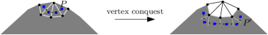
Figure 4. The effect of a conquest on $D$ is to delete a set of vertices $v_{1},\ldots,v_{r}$ together with their incident edges, denoted by $P=v_{1}\rightarrow v_{2}\ldots v_{r-1}\rightarrow v_{r}$. Call $D_{\mathrm{old}}$ the complex $D$ before conquest and call $D_{\mathrm{new}}$ the complex $D$ after conquest. As shown in the right picture, there is a neighboring path $P^{\prime}$ disjoint from $P$. Thanks to $P^{\prime}$, any path in $D_{\mathrm{old}}$ starting and ending out of $P$ and passing possibly by vertices and edges of $P$ can be modified into a path with same starting and ending vertices but not passing by $P$. Therefore $D_{\mathrm{new}}$ is connected.

The effect of the conquest on $D$ is shown in Figure 4; note that $D$ remains connected after the conquest. In addition, the number of boundary faces of $C$ is unchanged, as well as the Euler characteristic (indeed, if the number of faces transferred to $C$ is $k$, then the number of vertices transferred to $C$ is $k-1$ and the number of edges transferred to $C$ is $2k-1$). Therefore a conquer operation does not modify the topology of $C$.

3.2.2. Handle operators of second type

A chordal edge $e$ for $C$ is said to be separating if its dual edge $e^{*}$ is a bridge of $D$ (a bridge is an edge whose removal disconnects the graph). Otherwise it is called non-separating.

Definition 5 (split edge).

A split edge for $C$ is a non-separating chordal edge $e$ such that the two brins of $e$ are incident to boundary corners in the same boundary face of $C$.

According to the equivalence stated in Lemma 3, a split edge $e$ is such that $e^{*}$ is not a bridge but has the same boundary face (of $D$) on both sides.

We can now define the second operation, split, related to a split edge $e$: double $e$ into two parallel edges delimiting a face $f$ of degree $2$, and add the face $f$ and the two edges representing $e$ to $C$. Note that $D$ remains connected since $e^{*}$ is not a bridge. When doing the split operation, the boundary walk at the two extremities of $e$ is split into two boundary walks. Therefore the number of boundary faces of $C$ increases by $1$. Note that the Euler characteristic $\chi(C)$ decreases by $1$; indeed in $C$ the number of vertices is unchanged, the number of edges increases by $2$ (addition of the split edge, which is doubled) and the number of faces increases by $1$ (addition of the special face). And the Euler characteristic of the map $M$ associated with $C$ is unchanged (when including the boundary faces, the number of faces both increases by $2$, as the number of edges), hence the genus of $M$ is also unchanged.

Definition 6 (merge edge).

A merge edge for $C$ is a chordal edge having its two brins incident to boundary corners in distinct boundary faces of $C$.

According to Lemma 3, if $e$ is a merge edge, the faces of $D$ on both sides of $e^{*}$ are distinct boundary faces, hence $e^{*}$ cannot be a bridge of $D$, i.e., $e$ is non-separating.

We can now define the third operation, merge, related to a merge edge $e$: double $e$ into two parallel edges delimiting a face $f$ of degree $2$, and add the face $f$ and the two edges representing $e$ to $C$. Note again that $D$ remains connected since $e^{*}$ is not a bridge. When doing a merge operation, the boundary faces at the two extremities of $e$ are merged into a single boundary face, so that the number of boundary faces of $C$ decreases by $1$. Similarly as for a split operation, the Euler characteristic $\chi(C)$ decreases by $1$ (addition of a doubled special edge and of one special face); and the Euler characteristic of the map $M$ associated with $C$ decreases by $2$ (when including the boundary faces, the number of faces is unchanged, and the number of edges increases by $2$), hence the genus of $M$ increases by $1$; informally a merge operation “adds a handle”.

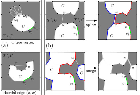
Figure 5. Illustrated on a toroidal graph, (a) the result of a conquer operation, and a contractible chordal edge $(u,w)$ (in gray); (b) the result of a split (respectively, merge) operation on a split edge $(u,w)$ (respectively, merge edge $(u,w)$).

4. Schnyder woods for triangulations of arbitrary genus

4.1. Definition of Schnyder Woods extended to arbitrary genus

We give here a definition of Schnyder woods for triangulations that extends to arbitrary genus the definition known in the planar case, see Figure 6 for an example. We consider here triangulations of genus $g$ with a marked face, called the root-face. As in the planar case, the edges and vertices are called outer or inner whether they are incident to the root-face or not.

Definition 7.

Consider a genus $g$ triangulation $\mathcal{T}$ with $n$ vertices, and having a root-face $f=(v_{0},v_{1},v_{2})$ (the vertices are ordered according to a walk along $f$ with the interior of $f$ on the right). Let $\mathcal{E}$ be the set of inner edges of $\mathcal{T}$. A $g$-Schnyder wood of $\mathcal{T}$ (also called genus $g$ Schnyder wood) is a partition of $\mathcal{E}$ into a set of normal edges and a set $\mathcal{E}^{s}$ of special edges considered as fat, i.e., each special edge is doubled into two edges delimiting a face of degree $2$, called a special face. In addition, each edge, a normal edge or one of the two edges of a special edge, is directed and has a label (also called color) in $\{0,1,2\}$, so as to satisfy the following conditions:

• root-face condition: The outer vertex $v_{2}$ is incident to no special edges. All inner edges incident to $v_{2}$ are ingoing of color $2$.

  Let $k\geq 0$ be the number of special edges incident to $v_{0}$ (each of these special edges is doubled), and let $L=(e_{1},f_{1},e_{2},f_{2},\ldots,e_{r},f_{r})$ be the cyclic list of edges and faces incident to $v_{0}$ in ccw order ($f_{i}$ is the face incident to $v_{0}$ between $e_{i}$ and $e_{(i+1)\ \mathrm{mod}\ r}$). A sector of $v$ is a maximal interval of $L$ that does not contain a special face nor the root-face. Note that there are $k+1$ sectors, which are disjoint; the one containing the edge $\{v_{0},v_{1}\}$ is called the root-sector.

  Then, all inner edges in the root-sector are ingoing of color $0$. In all the other $k$ sectors, the edges in ccw order are of the form

  $$\mathrm{Seq}(\mathrm{In}\ \!1),\mathrm{Out}\ \!0,\mathrm{Seq}(\mathrm{In}\ \!2),\mathrm{Out}\ \!1,\mathrm{Seq}(\mathrm{In}\ \!0).$$

  The definitions of sectors and conditions are the same for $v_{1}$, except that all edges in the root-sector are ingoing of color $1$.

• local condition for inner vertices: Every inner vertex $v$ has exactly one outgoing edge $e$ of color $2$. Let $k$ be the number of special edges incident to $v$ (each of these edges is doubled and delimits a special face), and let $L=(e_{1},f_{1},e_{2},f_{2},\ldots,e_{r},f_{r})$ be the cyclic list of edges and faces incident to $v$ in ccw order. A sector of $v$ is a maximal interval of $L$ that does not contain a special face nor the edge $e$. Note that there are $k+1$ sectors around $v$, which are disjoint.

  Then, in each sector the edges in ccw order are of the form

  $$\mathrm{Seq}(\mathrm{In}\ \!1),\mathrm{Out}\ \!0,\mathrm{Seq}(\mathrm{In}\ \!2),\mathrm{Out}\ \!1,\mathrm{Seq}(\mathrm{In}\ \!0).$$

• Cut-graph condition: The graph $T_{2}$ formed by the edges of color 2 is a tree spanning all vertices except $v_{0}$ and $v_{1}$, and rooted at $v_{2}$, i.e., all edges of $T_{2}$ are directed toward $v_{2}$. The embedded subgraph $G_{2}$ formed by $T_{2}$ plus the two edges $(v_{0},v_{2})$ and $(v_{1},v_{2})$ plus the special edges (not considered as doubled here) is a cut-graph of $\mathcal{T}$, which is called the cut-graph of the Schnyder wood.

(Note that the cut-graph condition forces the number of special edges to be $2g$.)

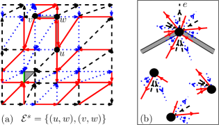
Figure 6. (a) A toroidal triangulation endowed with a $g$-Schnyder wood (the root-face is dashed). (b) The local condition for an inner vertex with two special edges (each of which is doubled and delimits a 2-sided face), below are shown the 3 sectors delimited by the special edges and the outgoing edge of color $2$.

As an example, Figure 6(a) shows a toroidal triangulation endowed with a g-Schnyder wood.

Remark 1. Note that if an inner vertex $v$ is incident to no special edge, then there is a unique sector around $v$, which is formed by all edges incident to $v$ except the outgoing one of color $2$. The local condition above implies that the edges around $v$ are of the form

$$(\mathrm{Seq}(\mathrm{In}\ \!1),\mathrm{Out}\ \!0,\mathrm{Seq}(\mathrm{In}\ \!2),\mathrm{Out}\ \!1,\mathrm{Seq}(\mathrm{In}\ \!0),\mathrm{Out}\ \!2),$$

as in the planar case. Since at most $4g$ vertices are incident to special edges, our definition implies that in fixed genus, almost all inner vertices satisfy the same local condition as in the planar case. In addition the vertices incident to special edges satisfy a local condition very similar to the one in the planar case.

Remark 2.

The last condition, stating that $T_{2}$ is a tree, is redundant in the planar case (it is implied by the local conditions) but not in higher genus: one easily finds an example of structure where all local conditions are satisfied but the edges of color $2$ form many disjoint circuits.

Remark 3.

Finally, we point out (see Proposition 14 and the remark after) that $g$-Schnyder woods (precisely, those computed by a traversal algorithm described later on) give rise to decompositions into 3 spanning cellular subgraphs, one with one face and the two other ones with $1+2g$ faces. This generalizes the decomposition of a plane triangulation into 3 spanning trees.

4.2. Computing Schnyder woods for any genus

This section presents an algorithm for traversing a triangulation of arbitrary genus $g\geq 0$ and computing a $g$-Schnyder wood on the way. Our algorithm naturally extends to any genus the procedure of Brehm. As in the planar case, the traversal is a greedy sequence of conquest operations, with here the important difference that these operations are interleaved with $2g$ merge/split operations. Another point is that, in higher genus, the region that is grown is more involved than in the planar case (recall that in the planar case, the grown region is delimited by a simple cycle). This is why we need the more technical terminology of subcomplex. It also turns out that a vertex might appear several times on the boundary of the grown complex, therefore we have to use the refined notion of free boundary corner, instead of free vertex in the planar case (in the planar case, a vertex appears just once on the boundary of the grown region).

Let us now give the precise description of the traversal procedure on a triangulation of genus $g$ with a root-face. As in the planar case, we grow a “region” $C$. Precisely, $C$ is a connected subcomplex all along the traversal. Initially, $C$ is the root-face $\{v_{0},v_{1},v_{2}\}$, together with the edges and vertices of that face; at the end, $C$ is equal to $\mathcal{T}$. We make use of the operation conquer$(b)$—with $b$ a free boundary corner of $C$—as defined in Section 3.2.1. Associated with such a conquest is the colorient rule, similar to the operation for free vertices described in Section 2.2 (planar case):

colorient

colorient($b$), with $b$ a free boundary corner of $C$: let $v$ be the vertex incident to $b$, and let $e$, $e^{\prime}$ be the two edges delimiting $b$, with $e^{\prime}$ after $e$ in cw order around $v$. Orient $e$ and $e^{\prime}$ outward of $v$, giving color $1$ to $e$ and color $0$ to $e^{\prime}$. Orient all the exterior edges of $b$ toward $v$ and give color $2$ to these edges (these edges are strictly between $e$ and $e^{\prime}$ in cw order around $v$).

We also make use of the handle operations split and merge, as defined in Section 3.2. Define an update-candidate for $C$ as either a free boundary corner, or a split edge, or a merge edge.

ComputeSchnyderAnyGenus($\mathcal{T}$) ($\mathcal{T}$ a triangulation of genus $g$)
Initialize $C$ as the root-face $f$ plus the vertices and edges of $f$;
while $C\neq\mathcal{T}$ find an update-candidate $\sigma$ for $C$
If $\sigma$ is a free boundary corner $b$
conquer($b$); colorient($b$);
If $\sigma$ is a merge edge $e=\{u,w\}$ for $C$
merge(u,w);
If $\sigma$ is a split edge $e=\{u,w\}$ for $C$
split(u,w);
end while

Note that the above algorithm performs conquests, merge operations, and split operations in whichever order, i.e., with no priority on the 3 types of operations.

Figure 8 shows the traversal algorithm executed on a toroidal triangulation. Observe the subtlety that, for positive genus, the vertices incident to merge/split edges have several corners that are conquered, as illustrated in Figure 7. Precisely, for a vertex $v$ incident to $k\geq 0$ merge/split edges, its conquest occurs $k+1$ times if $v$ is an inner vertex and $k$ times if $v\in\{v_{0},v_{1}\}$.

Note also that, if the algorithm terminates (which will be proved next), the number of merge edges must be $g$ and the number of split edges must be $g$. Indeed, in the initial step, $C$ has $k=1$ boundary face and genus $g^{\prime}=0$, while (just before) the last step $C$ has $k=1$ boundary face and genus $g^{\prime}=g$. Since the effect of each split is $\{k\leftarrow k+1,g^{\prime}\leftarrow g^{\prime}\}$ and the effect of each merge is $\{k\leftarrow k-1,g^{\prime}\leftarrow g^{\prime}+1\}$, there must be the same number of splits as merges (for $k$ to be the same finally as initially) and the number of merges must be $g$ (for $g^{\prime}$ to increase from $0$ to $g$). As we will see, these $2g$ edges are the special edges of the Schnyder wood computed by the traversal algorithm.

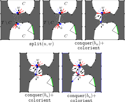
Figure 7. These pictures show the result of colorient operations in the higher genus case. Any split (or merge) edge $(u,w)$ can be directed in one or two directions (having possibly two colors), depending on the traversal order on its extremities (we denote by $b_{w}$ a boundary corner incident to vertex $w$).

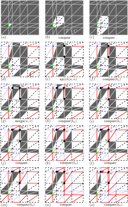
Figure 8. Execution of our traversal algorithm. (a) The traversal starts with a conquest at the outer vertex $v_{2}$. (b)-(c) As far as only $\mathtt{conquer}$ operations, (d) the area already explored (white triangles) remains homeomorphic to a disk. Whenever there remain no free corners, it is possible to find split (e) and merge (g) edges (incident to black circles). Once the region $\mathcal{T}\setminus C$ is a topological disk (h), the traversal can be completed with a sequence of conquer operations.

Theorem 8.

Any triangulation $\mathcal{T}$ of genus $g$ admits a $g$-Schnyder wood, which can be computed in time $O((n+g)g)$.

This theorem is proved in several steps: first we show in Lemma 9 that the traversal algorithm terminates and in Lemma 10 that it can be implemented to run in time $O((n+g)g)$. Then we show in Lemma 11 (local conditions) and Corollary 13 (cut-graph condition) that it computes a $g$-Schnyder wood.

4.3. Termination and complexity of the algorithm

Here $C$ denotes the growing subcomplex in the traversal algorithm, and $D$ denotes the complementary dual of $C$.

Lemma 9 (Termination).

Let $\mathcal{T}$ be a genus $g$ triangulation. Then at any step of ComputeSchnyderAnyGenus($\mathcal{T}$) strictly before termination, there is an update-candidate incident to the boundary face containing $\{v_{0},v_{1}\}$. Hence the procedure ComputeSchnyderAnyGenus($\mathcal{T}$) terminates.

Proof.

Consider the boundary face $f_{0}$ of $C$ containing the edge $\{v_{0},v_{1}\}$, at some step strictly before termination of the traversal. Assume that there is no split edge nor merge edge incident to $f_{0}$ (i.e., no split nor merge edge has one of its two extremities incident to a boundary corner of $f_{0}$): we are going to show that, in this case, there must be a free boundary corner incident to $f_{0}$. Each chordal edge $e$ incident to $f_{0}$ is separating. Hence $e$ is in fact incident to $f_{0}$ at its two extremities (otherwise $e$ would be a merge edge). Consider the complete list $L$ of brins around $f_{0}$, as defined in Section 3.1. Let $d$ and $e$ be any pair of chordal edges incident to $f_{0}$ (provided $f_{0}$ has at least two incident chordal edges). Note that $d^{*}$ and $e^{*}$ are bridges of $D$.

We claim that the brins $(d_{1},d_{2})$ of $d$ and $(e_{1},e_{2})$ of $e$ are not in a crossing-configuration, i.e., cannot appear as $(\ldots,d_{1},\ldots,e_{1},\ldots,d_{2},\ldots,e_{2},\ldots)$ in $L$. Indeed, if the order was so, Lemma 3 would imply that the dual brins appear as $(\ldots,e_{2}^{*},\ldots,d_{2}^{*},\ldots,e_{1}^{*},\ldots,d_{1}^{*},\ldots)$ in $\Phi(L)$. But this would imply that the dual edge $d^{*}$ of $d$ belongs simultaneously to the two connected components of $D\backslash e^{*}$.

Hence the cyclic boundary of $f_{0}$ (the contour of $f_{0}$ unfolded as a cycle) together with its chordal edges forms a planar chord-diagram with a root-edge $\{v_{0},v_{1}\}$, as shown in Figure 3. It is well known that, in such a diagram (as shown for instance by Brehm [7]), one can find a vertex $v\notin\{v_{0},v_{1}\}$ not incident to any chord. The corner at that vertex is hence free. ∎

Lemma 10 (Execution time).

The algorithm ComputeSchnyderAnyGenus($\mathcal{T}$) can be implemented to have running time $O((n+g)g)$—with $g$ the genus and $n$ the number of vertices of $\mathcal{T}$—and such that the update-candidate is always incident to the boundary face containing $\{v_{0},v_{1}\}$.

Proof.

At each step, call $f_{0}$ the boundary face of $C$ containing $\{v_{0},v_{1}\}$ and call $f_{0}^{*}$ the corresponding boundary face of $D$. Note that there are $2g$ merge/split operations during the execution of the algorithm. Accordingly, the execution time consists of $2g+1$ periods: each of the $2g$ first periods ends with a merge/split, and the last period finishes the traversal. To prove that the execution time is $O((n+g)g)$, it is enough to show that each period can be implemented to run in time $O(|E|)$, with $|E|$ the number edges of the triangulation (by the Euler relation, $|E|$ is $O(n+g)$). Our implementation here chooses always an update-candidate incident to $f_{0}$ and gives priority to free boundary corners over split and merge edges.

We manipulate maps using the half-edge data-structure; each brin has several pointers: to the incident vertex, the incident face, the opposite brin, the following brin, and the dual brin. There are fixed half-edge data structures for the triangulation $\mathcal{T}$ and for its dual $\mathcal{T}^{*}$, and there are evolving half-edge data-structures for $C$ and for the complementary dual $D$. Each brin of $D$ incident to a boundary face is dual to a brin exterior to a boundary corner of $C$. Accordingly such a brin of $D$ has an additional pointer to the corresponding boundary corner of $C$ (a boundary corner of $C$ is identified with a boundary brin of $C$) . And the brins of $D$ that are on an edge with a boundary face on both sides have a flag indicating this property; the dual of these edges are precisely the chordal edges for $C$. The boundary corners of $C$ have an additional parameter indicating the number of incident chordal edges. Hence, those that have this parameter equal to $0$ are the free boundary corners (except for the two corners at each extremity of $\{v_{0},v_{1}\}$). The free boundary corners incident to $f_{0}$ are stored in a list. As long as this list is not empty, one chooses the free boundary corner at the head of the list and performs the conquest/colorient operations. After performing a conquest, as shown in Figure 4, some edges of $D$ are deleted and some faces $f_{1},\ldots,f_{r}$ of $D$ are merged with a boundary face of $D$. The edges of $f_{1},\ldots,f_{r}$ that are not deleted are called uncovered by the conquest. Note that the only edges that might change status (i.e., become chordal) are the uncovered edges. If an uncovered edge $e$ becomes chordal (i.e., has now a boundary face of $D$ on both sides), one updates the status of $e$ as chordal, and accordingly one increments the parameter for the number of incident chordal edges of the boundary corners (for $C$) at the two extremities of the dual edge of $e$. Since an edge can be uncovered by at most two conquests and since the number of operations performed on an uncovered edge is constant, the complexity of updating the half-edge data structures over the whole period is $O(|E|)$.

At the end of a period, there is no free boundary corner incident to $f_{0}$. Hence, by Lemma 9, either the algorithm directly terminates, or there is a merge or split edge incident to $f_{0}$. To check for a merge edge incident to $f_{0}$, one scans the edges of $D$. If there is an edge $e\in D$ having distinct boundary faces on both sides and one of these faces is $f_{0}^{*}$, then one performs a merge operation at $e$, which finishes the period. Note that scanning all edges of $D$ in search of merge edges takes time $O(|E|)$.

If the traversal is not finished and one finds no merge edge incident to $f_{0}$, then by Lemma 9 there must be a split edge incident to $f_{0}$, i.e., an edge of $D$ that is not a bridge but has $f_{0}^{*}$ on both sides. One can find all the bridges of $D$ in $O(|E|)$ time using the depth-first search principles of Tarjan [39, 40]. Then one looks for a non-bridge edge $e$ of $D$ with $f_{0}^{*}$ on both sides, and performs a split operation at $e$, which finishes the period. Again this scanning process in search of a split edge takes time $O(|E|)$. ∎

4.4. The local conditions

We introduce some invariants on the colors and directions of the edges of a genus $g$ triangulation $\mathcal{T}$ that remain satisfied all along the traversal and ensure that the computed structure is a $g$-Schnyder wood.

In order to describe the invariants, we need to introduce some terminology. First we recall that the special edges are “fat”, i.e., considered as two parallel edges that delimit a face of degree 2 (this face is part of $C$ as soon as the special edge is in $C$). Given a vertex $v\in C$, let $L=(e_{1},f_{1},e_{2},f_{2},\ldots,e_{r},f_{r})$ be the sequence of edges and faces (which are either triangular or special) incident to $v$ in ccw order around $v$. In this list, the faces that are special (2-sided) are only those for special edges that are already in $C$. Let us first introduce two invariants that are easily checked to remain satisfied all along the traversal:

• The edges already colored and directed are those whose two incident faces are in $C$ (we include the special faces for the special edges already in $C$).

• Each inner vertex $v\in C$ has a unique outgoing edge of color $2$; the outer vertices do not have any outgoing edge of color $2$.

At each step, let $k$ be the number of special edges of $C$ incident to $v\in C$. If $v$ is an inner vertex of $\mathcal{T}$, define a sector as a maximal interval of $L$ that contains no special face nor the outgoing edge $e$ of color $2$. Note that $v$ has $k+1$ sectors, which are disjoint. A sector is called filled if all its faces are in $C$. We introduce the following invariants:

• Both faces incident to $e$ are in $C$.

• The edges in each filled sector are in ccw order:

  $$\mathrm{Seq}(\mathrm{In}\ \!1),\mathrm{Out}\ \!0,\mathrm{Seq}(\mathrm{In}\ \!2),\mathrm{Out}\ \!1,\mathrm{Seq}(\mathrm{In}\ \!0).$$

• In each non-filled sector the faces not in $C$ form an interval $I$ of faces around $v$. In ccw order in the sector, the directed/colored edges of $C$ before $I$ are ingoing of color $1$, and the directed/colored edges of $C$ after $I$ are ingoing of color $0$.

Similarly we define an invariant for $v_{2}$ (which is true from the first conquest):

• All inner edges incident to $v_{2}$ are non-special and are ingoing of color $2$.

Finally we define invariants for $v_{0}$ (and similarly for $v_{1}$). At each step, let $k$ be the number of special edges of $C$ that are incident to $v_{0}$. Let $L=(e_{1},f_{1},e_{2},f_{2},\ldots,e_{r},f_{r})$ be the sequence of edges and faces (which are triangular or special) incident to $v_{0}$ in ccw order around $v_{0}$ (again, the special faces are those for special edges already in $C$). Define a sector as a maximal interval of $L$ that contains no special face nor the root-face. Note that $v$ has $k+1$ sectors, which are disjoint; the one containing the edge $\{v_{0},v_{1}\}$ is called the root-sector. Again a sector is called filled if all its faces are in $C$. We introduce the following invariants:

• In each sector the faces not in $C$ form an interval $I$ of faces around $v_{0}$.

• The non-root face incident to $\{v_{0},v_{1}\}$ is never in $C$ strictly before termination. Hence the root-sector is never filled strictly before termination. All the colored/directed edges in the root-sector are going toward $v_{0}$ and have color $0$.

• The edges in each filled non-root sector are in ccw order:

  $$\mathrm{Seq}(\mathrm{In}\ \!1),\mathrm{Out}\ \!0,\mathrm{Seq}(\mathrm{In}\ \!2),\mathrm{Out}\ \!1,\mathrm{Seq}(\mathrm{In}\ \!0).$$

• In ccw order in a non-filled non-root sector, the directed/colored edges of $C$ before $I$ are ingoing of color $1$, and the directed/colored edges of $C$ after $I$ are ingoing of color $0$.

The invariants are the same for $v_{1}$, except that the colored/directed edges in the root-sector are going toward $v_{1}$ and have color $1$.

One easily checks that these invariants remain satisfied after each conquest, split, or merge operation.

Lemma 11.

The structure computed by ComputeSchnyderAnyGenus($\mathcal{T}$) satisfies the local conditions of a $g$-Schnyder wood.

Proof.

At the end, the fact that the invariants are satisfied directly implies that the local conditions for edge directions and colors of a $g$-Schnyder wood are satisfied. ∎

4.5. The cut-graph property.

Let $\mathcal{T}$ be a genus $g$ triangulation on which the traversal algorithm is applied. Let $G_{2}$ be the graph formed by the edges of color $2$, the two edges $\{v_{1},v_{2}\}$ and $\{v_{0},v_{2}\}$, and the $2g$ special edges, not considered as doubled here.

Lemma 12.

At each step strictly before the end of the traversal algorithm, let $M$ be the map associated with $C$ and let $G_{2}^{\prime}$ be the embedded subgraph of $G_{2}$ consisting of the edges and vertices of $G_{2}$ that are in $C$.

Then $G_{2}^{\prime}$ is a cellular spanning subgraph of $M$. In addition there is a natural bijection between the faces of $G_{2}^{\prime}$ and the boundary faces of $M$: each boundary face of $M$ is included in a unique face of $G_{2}^{\prime}$.

Proof.

First let us observe that $G_{2}^{\prime}$ is a cellular spanning subgraph of $M$ iff it is connected, spanning, and has the same genus as $M$.

The property is true initially. Indeed, $C$ is the root-face, which is planar, so $M$ is the triangulation of the sphere with one inner face and one root-face, which plays the role of the boundary face; whereas $G_{2}^{\prime}$ consists of the two edges $\{v_{1},v_{2}\}$ and $\{v_{0},v_{2}\}$, so $G_{2}^{\prime}$ is a spanning tree of $M$.

Let $k$ be the number of boundary faces of $M$, which is also the number of faces of $G_{2}^{\prime}$, and let $g^{\prime}$ be the common genus of $M$ and $G_{2}^{\prime}$ before an operation is performed. Let us prove that the property stated in the lemma remains true after the operation, whether a conquest (except the last conquest), a merge, or a split.

Consider a conquest of a free boundary corner $b$, strictly before the very last conquest (which closes $C$). The new vertices appearing in $C$ are connected to the former graph $G_{2}^{\prime}$ by an outgoing edge of color $2$ in the new graph $G_{2}^{\prime}$, hence $G_{2}^{\prime}$ is still a connected spanning subgraph of $C$ after the conquest. Note also that the genera of $M$ and $G_{2}^{\prime}$ are unchanged (these two numbers stay equal to $g^{\prime}$). Similarly the number of boundary faces of $M$ and the number of faces of $G_{2}^{\prime}$ are unchanged (these two numbers stay equal to $k$). Finally, as shown in Figure 9, the boundary face of $M$ incident to $b$ is still contained in the corresponding face of $G_{2}^{\prime}$ after the conquest. Hence the property stated in the lemma remains true after a conquest.

Now let us consider a split operation. The new split edge “splits” a boundary face of $M$ into two faces $f_{1}$ and $f_{2}$, and in the same way splits the corresponding face of $G_{2}^{\prime}$ into two faces $f_{1}^{\prime}$ and $f_{2}^{\prime}$ such that $f_{1}^{\prime}$ contains $f_{1}$ and $f_{2}^{\prime}$ contains $f_{2}$. Thus the correspondence between boundary faces of $M$ and faces of $G_{2}^{\prime}$ remains true. In addition, the genera of $M$ and of $G_{2}^{\prime}$ remain unchanged, equal to $g^{\prime}$, hence $G_{2}^{\prime}$ remains a cellular subgraph of $M$, and is still spanning (no vertex is added to $M$ nor to $G_{2}^{\prime}$). Hence the property remains true after a split.

Finally consider a merge. The new merge edge “merges” two boundary faces $f_{1}$ and $f_{2}$ of $M$ into a single face, thereby adding a handle (informally, the handle serves to establish a bridge so as to connect and merge the two faces). Doing this the two corresponding faces $f_{1}^{\prime}$ and $f_{2}^{\prime}$ of $G_{2}^{\prime}$ are also merged into a single face that contains the merger of $f_{1}$ and $f_{2}$, see Figure 10. Thus the correspondence between boundary faces of $M$ and faces of $G_{2}^{\prime}$ remains true. In addition, the genera of $M$ and of $G_{2}^{\prime}$ both increase by $1$, they are equal to $g^{\prime}+1$ after the merge, so $G_{2}^{\prime}$ remains a cellular subgraph of $M$, and is still spanning (no vertex is added to $M$ nor to $G_{2}^{\prime}$). Hence the property remains true after a merge. ∎

Corollary 13.

The graph $G_{2}$ is a cut-graph of $\mathcal{T}$.

Proof.

Before the very last conquest, $G_{2}^{\prime}$ becomes equal to $G_{2}$; and $C$ is equal to $\mathcal{T}$ minus the triangular face $f$ on the other side of the root-face from the base-edge $\{v_{0},v_{1}\}$. Hence the map $M$ associated with $C$ is equal to $\mathcal{T}$, up to marking $f$ as a boundary face. According to Lemma 12, $G_{2}^{\prime}=G_{2}$ is a spanning cellular subgraph of $M=\mathcal{T}$ and has a unique face (since $M$ has a unique boundary face), hence $G_{2}$ is a cut-graph of $\mathcal{T}$. ∎

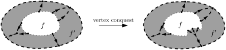
Figure 9. A conquest of a free boundary corner shrinks the interior of a boundary face $f$ (contour in dotted lines) as well as the interior of the face $f^{\prime}$ (contour in dashed lines) of $G_{2}^{\prime}$ that contains $f$ (for the sake of clarity, the faces of $C$ are shaded in this figure). The inclusion $f\subset f^{\prime}$ remains true after the conquest.

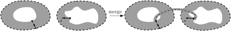
Figure 10. The effect of a merge operation on the growing subcomplex $C$ and on $G_{2}^{\prime}$ (the faces of $C$ are shaded in this figure). Two faces of $G_{2}^{\prime}$ are merged and the two corresponding boundary faces of $C$ are merged (the contours of the boundary faces of $C$ are dotted while the contours of the faces of $G_{2}^{\prime}$ are dashed).

4.6. The graphs in color $0$ and $1$ are also cellular

In this section we show that a $g$-Schnyder wood computed by the traversal algorithm yields a decomposition of a triangulation into 3 spanning cellular subgraphs $G_{0}$, $G_{1}$, $G_{2}$, with $G_{2}$ having one face ($G_{2}$ is the cut-graph of the Schnyder wood) and $G_{0}$ and $G_{1}$ having each $1+2g$ faces. This is a natural extension of the property that a planar Schnyder wood yields a decomposition of a plane triangulation into 3 spanning trees.

Proposition 14.

Let $\mathcal{T}$ be a triangulation of genus $g$ endowed with a $g$-Schnyder wood computed by the algorithm ComputeSchnyderAnyGenus. The special edges are doubled (thus $\mathcal{T}$ gets $2g$ additional degenerated faces of degree 2).

Let $G_{0}$ be the graph formed by the edges with color $0$ plus the outer edges incident to $v_{0}$. Then $G_{0}$ is a spanning cellular subgraph of $\mathcal{T}$ with $1+2g$ faces (where some of the faces might be degenerated, of degree 2). Similarly the graph $G_{1}$ formed by the edges of color $1$ plus the two outer edges incident to $v_{1}$ is a spanning cellular subgraph of $\mathcal{T}$ with $1+2g$ faces.

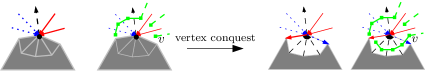
Figure 11. The effect of a conquest on the complementary dual $D_{0}$ of $G_{0}$ is to attach a chain at a vertex $v$, hence $D_{0}$ remains acyclic.

Proof.

By the local conditions of $g$-Schnyder woods, $G_{0}$ spans all inner vertices (each such vertex is incident to at least one edge of color $0$). Since one adds the two edges $\{v_{0},v_{2}\}$ and $\{v_{0},v_{1}\}$, $G_{0}$ also spans the vertices of the root-face, so $G_{0}$ is a spanning subgraph of $\mathcal{T}$. Let $\mathcal{T}^{*}$ be the dual map of $\mathcal{T}$. To show that $G_{0}$ is cellular, it is enough to show that the complementary dual $D_{0}$ of $G_{0}$ is acyclic ($D_{0}$ is the subgraph of $\mathcal{T}^{*}$ induced by all vertices of $\mathcal{T}^{*}$ and by the edges of $\mathcal{T}^{*}$ that are dual to the edges of $\mathcal{T}\setminus G_{0}$). At each step of the traversal algorithm, let $D_{0}^{\prime}$ be the subgraph of $D_{0}$ induced by the edges of $D_{0}$ dual to edges having a face in $C$ on both sides. Let us show that $D_{0}^{\prime}$ remains acyclic (i.e., a forest) all along the traversal algorithm. The effect of a merge or split is to add to $C$ a special edge $e$, precisely, the two edges representing $e$ and the 2-sided enclosed face. Since the two triangular faces incident to each side of $e$ are not in $C$, a merge or a split does not add any edge to $D_{0}^{\prime}$, so $D_{0}^{\prime}$ remains acyclic. Now consider a conquest of a free boundary corner $b$. Before the conquest, let $e$ and $e^{\prime}$ be the edges delimiting $b$ in cw order, let $f$ be the face encountered just before $e$ in cw order around the origin of $b$, and let $v$ be the vertex of $D_{0}^{\prime}$ corresponding to $f$. Then, as shown in Figure 11, the effect of the conquest on $D_{0}^{\prime}$ is to attach a chain at $v$. Hence $D_{0}^{\prime}$ remains acyclic. At the end, $D_{0}^{\prime}$ is equal to $D_{0}$, hence $D_{0}$ is acyclic, so $G_{0}$ is cellular. Finally, $G_{0}$ has $n$ vertices ($G_{0}$ spans all vertices of $\mathcal{T}$) and has $n+4g-1$ edges according to the local conditions. Since $G_{0}$ has genus $g$, the Euler relation ensures that $G_{0}$ has $1+2g$ faces. The proof for $G_{1}$ relies on the same arguments. ∎

Remark 5. The properties of $G_{2}$ (cut-graph condition), and of $G_{0}$, $G_{1}$ (stated in Proposition 14) can be considered as extensions of the fundamental property of planar Schnyder woods [37, 38]: in the planar case, for each color $i\in\{0,1,2\}$, the graph formed by the edges in color $i$ plus the two outer edges incident to $v_{i}$ is a spanning tree. Figure 12 shows an example in genus $1$.

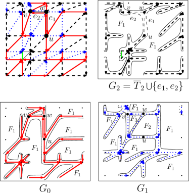
Figure 12. A triangulated torus endowed with a Schnyder wood. The dashed edges (color $2$) form a tree $T_{2}$, and the addition of the two special edges and the two outer edges incident to $v_{2}$ yields a cut-graph $G_{2}$. The solid edges (color $0$) plus the two outer edges incident to $v_{0}$ form a spanning cellular subgraph $G_{0}$ with $3$ faces (one face having degree $2$). Similarly, the solid edges (color $1$) plus the two outer edges incident to $v_{1}$ form a spanning cellular subgraph $G_{1}$ with $3$ faces.

5. Application to encoding

In the planar case, Schnyder woods yield a simple encoding procedure for triangulations, as described in [24] and more recently in [2]. Precisely, a planar Schnyder wood with $n$ vertices is encoded by two parenthesis words $W,W^{\prime}$ of respective lengths $2n-2$ and $2n-6$. Let $\overline{T_{2}}$ be the tree $T_{2}$ plus the two outer edges incident to $v_{2}$. Call $\theta$ the corner incident to $v_{2}$ in the outer face. The first word $W$ is the parenthesis word (also called Dyck word) that encodes the tree $\overline{T_{2}}$, that is, $W$ is obtained from a cw walk (i.e., the walker has the infinite face on its right) around $\overline{T_{2}}$ starting at $\theta$, writing an opening parenthesis at the first traversal of an edge of $\overline{T_{2}}$ (away from the root) and a closing parenthesis at the second traversal (toward the root). The second word $W^{\prime}$ is obtained from the same walk around $T_{2}$, but $W^{\prime}$ encodes the edges that are not in $\overline{T_{2}}$, i.e., the edges of color $0$ and $1$. Precisely, during the traversal, write an opening parenthesis in $W^{\prime}$ each time an outgoing edge in color $0$ is crossed and write a closing parenthesis in $W^{\prime}$ each time an ingoing edge of color $1$ is crossed.

For a triangulation with $n$ vertices, $W$ has length $2n-2$, and $W^{\prime}$ has length $2n-6$. Hence the coding word has total length $4n-8$. This code is both simple and quite compact, as the length $4n-8$ is not far from the information-theory lower bound of $\log_{2}\left(4^{4}/3^{3}\right)\approx 3.245$ bits per vertex, which is attained in the planar case by a bijective construction due to Poulalhon and Schaeffer [33].

In the higher genus case there does not exist an exact enumeration formula, nevertheless an asymptotic estimate [23] of the number of genus $g$ rooted triangulations with $n$ vertices leads to the information theory lower bound of $3.245n+\Omega(g\log n)$, i.e., the exponential growth rate is the same in every genus. For the higher genus case we do not yet know any linear time encoding algorithm matching asymptotically the information theory bound, and a bijective construction based on a special spanning tree is still to be found. Nevertheless we can here extend to higher genus the simple encoding procedure of [24, 2] based on Schnyder woods.

Encoding in higher genus

To encode the Schnyder wood we proceed in a similar way as in the planar case except that we have to deal with the special edges. Let $\mathcal{T}$ be a genus $g$ triangulation with $n$ vertices endowed with a Schnyder wood computed by our traversal algorithm; precisely, we use the implementation described in Lemma 10. Let $\overline{T_{2}}$ be the spanning tree of $\mathcal{T}$ consisting of the edges in color $2$ plus the two edges $\{v_{0},v_{2}\}$ and $\{v_{1},v_{2}\}$. Let $G_{2}$ be the cut-graph of the Schnyder wood, i.e., $G_{2}$ is $\overline{T_{2}}$ plus the $2g$ special edges. We classically encode $G_{2}$ as the Dyck word $W$ for $\overline{T_{2}}$, augmented by $2g$ memory blocks, each of size $O(\log(n))$ bits, so as to locate the two extremities of each special edge. In each memory block we also store the colors and directions of the two sides of the special edge. Hence $G_{2}$ is encoded by a word $W$ of length $2n-2+O(g\log(n))$. The encoding of the Schnyder wood is completed by a second binary word $W^{\prime}$ that is obtained from a clockwise walk along the (unique) face of $G_{2}$ (cw means that the face is on the right of the walker) starting at the corner $\theta$ incident to $v_{2}$ in the root-face. Along this walk, we write a $0$ when crossing a non-special outgoing edge of color $0$ and we write a $1$ when crossing a non-special ingoing edge of color $1$. Since there are $2n-6+4g$ non-special edges of color $0$ or $1$, the word $W^{\prime}$ has length $2n-6+4g$. Therefore the pair of words $(W,W^{\prime})$ is of total length $4n+O(g\log(n))$. In addition these words can be obtained in time $O((n+g)g)$ from a Schnyder wood on $\mathcal{T}$ (as we have seen in Lemma 10, the Schnyder wood itself can be computed in time $O((n+g)g)$.

Now we are going to show that the pair $(W,W^{\prime})$ actually encodes the Schnyder wood (and in particular the triangulation) and that the Schnyder wood can be reconstructed from $(W,W^{\prime})$ in time $O((n+g)g)$. The proof relies on two lemmas.

Lemma 15.

Let $\mathcal{T}$ be a triangulation endowed with a $g$-Schnyder wood. Then the Schnyder wood can be recovered after the deletion process that consists in removing all the non-special edges of color 0. In other words, the information given by non-special edges of color 0 is redundant.

Proof.

To have a unified treatment (no special case for the vertex $v_{0}$) it proves convenient here to direct the edges $\{v_{0},v_{2}\}$ and $\{v_{0},v_{1}\}$ out of $v_{0}$ and to give color $2$ to $\{v_{0},v_{2}\}$ and color $1$ to $\{v_{0},v_{1}\}$. Consider a maximal non-empty interval $I$ of non-special edges of color $0$ going into a vertex $v$ of $\mathcal{T}$. Let $e$ and $e^{\prime}$ be the edges that respectively precede and follow $I$ in cw order around $v$. By the local conditions of Schnyder woods (Figure 6(b)), $e^{\prime}$ is outgoing of color $1$; and either $e$ belongs to a special edge and is ingoing of color $0$, or $e$ is outgoing of color $2$. Let $P=v_{0},v_{1},\ldots,v_{k},v_{k+1}$ be the path of $\mathcal{T}$ formed by the neighbors of $v$ in cw order between $e$ and $e^{\prime}$, that is, $v_{0}$ is the other end of $e$, $v_{k+1}$ is the other end of $e^{\prime}$, and the $v_{i}$’s for $1\leq i\leq k$ are the other ends of the edges of $I$ taken in cw order around $v$. Then, by the local conditions of Schnyder woods, each edge $\{v_{i},v_{i+1}\}$, for $0\leq i\leq k$, either is of color $1$ directed from $v_{i}$ to $v_{i+1}$ or is of color $2$ directed from $v_{i+1}$ to $v_{i}$. Hence, the edges of $P$ and the edges $e$ and $e^{\prime}$ are not removed by the deletion process. Call $M$ the map created from $\mathcal{T}$ by the deletion process. Then there is a face $f$ in $M$ delimited by $P$, $e$ and $e^{\prime}$: this is the face of $M$ formed by the removal of the edges in $I$. In addition the corner formed by $e$ and $e^{\prime}$ is the unique corner of $f$ whose right-edge (looking toward the interior of $f$) is outgoing of color $1$. Thus the edges removed inside $f$ (and more generally all the removed edges) can be recovered: one looks for the unique corner of $f$ whose right-edge is outgoing of color $1$, and then one inserts an interval of ingoing edges of color $0$ at the corner so as to triangulate $f$. ∎

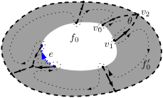
Figure 13. An edge $e$ colored $1$ (dotted arc) has the boundary face $f_{0}$ on its right just before the conquest coloring $e$. Hence, just before the conquest, a cw walk around $f_{0}^{\prime}$ (dashed lines) encounters the outgoing brin of $e$ first.

Lemma 16.

Consider a $g$-Schnyder wood $S$ calculated by the traversal algorithm under the implementation described in Lemma 10. Denote by $G_{2}$ the cut-graph of $S$ and by $\theta$ the corner incident to $v_{2}$ in the root-face ($\theta$ is also a corner of $G_{2}$). Let $e$ be a non-special edge of color $1$ of $S$.

Then, during a cw walk along $G_{2}$ (i.e., with the unique face of $G_{2}$ on the right of the walker) starting at $\theta$, the outgoing brin of $e$ is crossed before the ingoing brin of $e$.

Proof.

At each step of ComputeSchnyderAnyGenus strictly before termination, let $f_{0}$ be the boundary face of $C$ containing $\{v_{0},v_{1}\}$ and let $f_{0}^{\prime}$ be the corresponding face of $G_{2}^{\prime}$ (we use the notation of Lemma 12, $G_{2}^{\prime}$ consists of the edges and vertices of $G_{2}$ that are in $C$), that is, $f_{0}^{\prime}$ is the face of $G_{2}^{\prime}$ containing $f_{0}$. An edge $e$ of color $1$ has $f_{0}$ on its right just before the conquest coloring $e$ (by definition of the colorient rule). Hence, as shown in Figure 13, $e$ is encountered first at its outgoing brin during a cw walk around $f_{0}^{\prime}$ starting at $\theta$; and this property will continue to hold for $e$ until the end of the traversal.

∎

We can now describe how to reconstruct the Schnyder wood from the two words $(W,W^{\prime})$. First, construct the cut-graph $G_{2}$ using $W$. Note that the directions of edges and colors of the two sides of each special edge of $G_{2}$ are known from $W$. Hence, by the local conditions of Schnyder woods, we can already insert the outgoing brins of color $0$ or $1$ that are non-special (a non-special brin is a brin of a non-special edge). The non-special outgoing brins of color $0$ are ordered as $b_{1},b_{2},\ldots,b_{k}$ according to the order in which they are crossed during a cw walk along $G_{2}$ (i.e., with the unique face of $G_{2}$ on the right of the walker). Next, the word $W^{\prime}$ indicates where to insert the non-special ingoing brins of color $1$. Precisely, factor $W^{\prime}$ as

$$W^{\prime}=1^{\!r_{1}}01^{\!r_{2}}01^{\!r_{3}}\ldots 01^{\!r_{k+1}},$$

where the integers $r_{i}$’s are allowed to be zero. Then, for each $i\in[1..k]$, insert $r_{i}$ ingoing brins of color $1$ in the corner $(b_{i},\mathrm{follower}(b_{i}))$ (where the follower of a brin $b$ is the next brin after $b$ in cw order around its origin). And insert $r_{k+1}$ ingoing brins of color $1$ in the corner incident to $v_{1}$ delimited to the right by $\{v_{1},v_{0}\}$.

Afterwards, we use Lemma 16 to form the non-special edges of color $1$. Write a parenthesis word $\pi$ obtained from a cw walk along $G_{2}$ starting at $\theta$, writing an opening parenthesis each time a non-special outgoing brin of color $1$ is crossed and writing a closing parenthesis each time a nonspecial ingoing brin of color $1$ is crossed. Then, Lemma 16 ensures that the matchings of $\pi$ correspond to the non-special edges of color $1$ in the Schnyder wood, so we just have to form the non-special edges of color $1$ according to the matchings of $\pi$.

Finally, since the edges of color $0$ are redundant (by Lemma 15), there is no ambiguity to insert the edges of color $0$ at the end (i.e., complete the already inserted outgoing half-edges of color $0$ into edges).

To conclude, the non-special edges of color $0$ are redundant, the cut-graph can be encoded by a parenthesis word $W$ of length $2n-2$ (for the tree $\overline{T_{2}}$) plus $O(g\log(n))$ bits of memory for the special edges, and the edges of color $1$ can be inserted from a word $W^{\prime}$ of length $2n-6+4g$. Clearly the reconstruction of the Schnyder wood from $(W,W^{\prime})$ takes time $O((n+g)g)$, since it just consists in building the cut-graph $G_{2}$ and walking cw along $G_{2}$. All in all, we obtain the following result:

Proposition 17.

A triangulation of genus $g$ with $n$ vertices can be encoded—via a $g$-Schnyder wood—by a binary word of length $4n+O(g\log(n))$. Coding and decoding can be done in time $O((n+g)g)$.

We mention that one could also design a more sophisticated code that supports queries, as done in [14, 1]. The arguments would be similar to the ones given in [1], which treats plane (labeled) triangulations. To wit, given a genus $g$ (unlabeled) triangulation $\mathcal{T}$ with $f$ faces and $e$ edges, one could obtain a compact representation of $\mathcal{T}$ using asymptotically $(2\log 6)e+O(g\log e)$ bits, or equivalently $7.755\ \!f+O(g\log f)$ bits, which answers queries for vertex adjacency and vertex degree in $O(1)$ time. The main idea would be to compute a g-Schnyder wood of $\mathcal{T}$ and to encode the corresponding maps $G_{i}$, $i\in\{0,1,2\}$. In order to efficiently support adjacency queries on vertices, we would have to encode the three maps $G_{0}$, $G_{1}$, $G_{2}$ using a multiple parenthesis system (3 types of parentheses).

In [9] is described another partitioning strategy (not based on Schnyder woods nor canonical orderings) answering queries, which achieves a better compression rate of $2.175f+O(g\log f)$ bits when dealing with genus $g$ triangulations having $f$ triangles (using a different face-based navigation). Nevertheless, we believe that, compared to [9], an approach based on Schnyder woods would make it possible to deal in higher genus with more general graphs ([14]) and labeled graphs (as done in [1] in the planar case).

6. Conclusion and perspectives

We have extended to arbitrary genus the definition of Schnyder woods, a traversal procedure for computing such a Schnyder wood in linear time (for fixed genus) and an encoding algorithm providing an asymptotic compression rate of $4$ bits per vertex (again for fixed genus). Some further problems and related topics are listed next.

Applications of Schnyder Woods as canonical orderings

We point out that our graph traversal procedure induces an ordering for treating the vertices so as to shell the surface progressively. Such an ordering is already well known in the planar case under the name of canonical ordering and has numerous applications for graph encoding and graph drawing [14, 25]. It is thus of interest to extend this concept to higher genus. The only difference is that in the genus $g$ case there is a small number —at most $2\cdot 2g$— of vertices that might appear several times in the ordering; these correspond to the vertices incident to the $2g$ special edges (split/merge edges) obtained during the traversal. There are several open questions we think should be investigated concerning the combinatorial properties of such orderings and the corresponding edge orientations and colorations. A related question in our context is to ask if any Schnyder wood can be obtained as a result of our traversal procedure (if not, which property the Schnyder wood has to satisfy). Another line of research is to see whether such an ordering would yield an efficient algorithm for drawing a graph on a genus $g$ surface (as it has been done in the planar case [25]).

Further extensions

Our approach relies on quite general topological and combinatorial arguments, so the natural next step should be to apply our methodology to other interesting classes of graphs (not strictly triangulated), which have similar characterization in the planar case. Our topological traversal could be extended to the $3$-connected case, precisely to embedded 3-connected graphs with face-width larger than 2, which correspond to polygonal meshes of genus $g$. We point out that our encoding proposed in Section 5 could take advantage of the existing compact encodings of planar graphs [14, 13, 24], using similar parenthesis-based approaches.

Lattice structure and graph encoding applications

From the combinatorial point of view it should be of interest to investigate whether edge orientations and colorations in genus $g$ have nice lattice properties, as in the planar case. In the planar case, so-called minimal $\alpha$-orientations have a deep combinatorial role (they yield bijective constructions for several families of planar maps, including triangulations), and as such, have also applications in graph drawing, random sampling, and coding [33].

In the planar case, as shown by Brehm [7], the minimal Schnyder wood is reached by a “left-most driven” traversal of the triangulation, and is computable in linear time. We would like to extend these principles to any genus and derive from it a linear time encoding procedure with (asymptotically) optimal compression rate. Hopefully these principles can also be applied to polygonal meshes of arbitrary genus.

Acknowledgments.

We are grateful to Nicolas Bonichon, Cyril Gavoille and Arnaud Labourel for very interesting discussions on Schnyder woods. First author would like to thank Éric Colin de Verdière for pointing out some useful topological properties of graphs on surfaces. We are extremely grateful to Olivier Bernardi, Guillaume Chapuy, and Gilles Schaeffer for enlightening discussions on the combinatorics of maps that motivated this work and helped to clarify the ideas. We finally thank the reviewers for their very insightful remarks. The first two authors’ work was partially supported by ERC research starting grant ”ExploreMaps”. The last author would like to thank CNPq and FAPERJ for financial support.

References

- [1] J. Barbay, L. Castelli-Aleardi, M. He, and J. I. Munro. Succinct representation of labeled graphs. In ISAAC, pages 316–328, 2007.
- [2] O. Bernardi and N. Bonichon. Intervals in Catalan lattices and realizers of triangulations. Journal of Combinatorial Theory - Series A, Vol 116(1) pp 55-75, 2009.
- [3] N. Bonichon. Aspects algorithmiques et combinatoires des réaliseurs des graphes plans maximaux. PhD thesis, Bordeaux I, 2002.
- [4] N. Bonichon, C. Gavoille, and N. Hanusse. An information-theoretic upper bound of planar graphs using triangulation. In STACS, pages 499–510. Springer, 2003.
- [5] N. Bonichon, C. Gavoille, N. Hanusse, D. Poulalhon, and G. Schaeffer. Planar graphs, via well-orderly maps and trees. Graphs and Combinatorics, 22(2):185–202, 2006.
- [6] N. Bonichon, C. Gavoille, and A. Labourel. Edge partition of toroidal graphs into forests in linear time. In ICGT, volume 22, pages 421–425, 2005.
- [7] E. Brehm. -orientations and Schnyder-three tree decompositions. Master’s thesis, Freie Universität Berlin, 2000.
- [8] S. Cabello and B. Mohar. Finding shortest non-separating and non-contractible cycles for topologically embedded graphs. Discrete & Comp. Geometry, 37(2):213–235, 2007.
- [9] L. Castelli-Aleardi, O. Devillers, and G. Schaeffer. Succinct representation of triangulations with a boundary. In WADS, pages 134–145. Springer, 2005.
- [10] L. Castelli-Aleardi, O. Devillers, and G. Schaeffer. Succinct representations of planar maps. In Theoretical Computer Science, 408:174-187, 2008. (preliminary version in SoCG’06)
- [11] G. Chapuy. Asymptotic enumeration of constellations and related families of maps on orientable surfaces. arXiv:0805.0352, 2008.
- [12] G. Chapuy, M. Marcus, and G. Schaeffer. A bijection for rooted maps on orientable surfaces. arXiv:0712.3649, 2007.
- [13] Y.-T. Chiang, C.-C. Lin, and H.-I. Lu. Orderly spanning trees with applications to graph encoding and graph drawing. In SODA, pages 506–515, 2001.
- [14] R. C.-N. Chuang, A. Garg, X. He, M.-Y. Kao, and H.-I. Lu. Compact encodings of planar graphs via canonical orderings and multiple parentheses. ICALP, pages 118–129, 1998.
- [15] H. de Fraysseix and P. O. de Mendez. On topological aspects of orientations. Discrete Mathematics, 229:57–72, 2001.
- [16] P. O. de Mendez. Orientations bipolaires. PhD thesis, Paris, 1994.
- [17] É. C. de Verdière and F. Lazarus. Optimal system of loops on an orientable surface. In Discrete & Computational Geometry, 33(3):507-534, 2005. (preliminary version in FOCS’02)
- [18] J. Erickson and S. Har-Peled. Optimally cutting a surface into a disk. Discrete & Computational Geometry, 31(1):37–59, 2004.
- [19] S. Felsner. Convex drawings of planar graphs and the order dimension of -polytopes. Order, 18:19–37, 2001.
- [20] S. Felsner. Lattice structures from planar graphs. Electronic Journal of Combinatorics, 11(15):24, 2004.
- [21] É. Fusy. Combinatoire des cartes planaires et applications algorithmiques. PhD thesis, Ecole Polytechnique, 2007.
- [22] É. Fusy, D. Poulalhon, and G. Schaeffer. Dissections, orientations, and trees with applications to optimal mesh encoding and random sampling. In ACM Transactions on Algorithms, 4(2), 2008. (preliminary version in SODA’05)
- [23] Z. Gao. A pattern for the asymptotic number of rooted maps on surfaces. Journal of Combinatorial Theory, Series A, 64:246–264, 1993.
- [24] X. He, M.-Y. Kao, and H.-I. Lu. Linear-time succinct encodings of planar graphs via canonical orderings. SIAM Journal on Discrete Mathematics, 12:317–325, 1999.
- [25] G. Kant. Drawing planar graphs using the canonical ordering. Algorithmica, 16(1):4–32, 1996.
- [26] K. Keeler and J. Westbrook. Short encodings of planar graph and maps. Discrete and Applied Mathematics, 58:239–252, 1995.
- [27] M. Kutz. Computing shortest non-trivial cycles on orientable surfaces of bounded genus in almost linear time. In SoCG, pages 430–438, 2006.
- [28] F. Lazarus, M. Pocchiola, G. Vegter, and A. Verroust. Computing a canonical polygonal schema of an orientable triangulated surface. In SoCG, pages 80–89, 2001.
- [29] T. Lewiner, H. Lopes, J. Rossignac, and A. W. Vieira. Efficient edgebreaker for surfaces of arbitrary topology. In Sibgrapi, pages 218–225, 2004.
- [30] T. Lewiner, H. Lopes, and G. Tavares. Optimal discrete Morse functions for 2-manifolds . Computational Geometry, 26(3): 221-233, 2003.
- [31] H. Lopes, J. Rossignac, A. Safonova, A. Szymczak, and G. Tavares. Edgebreaker: a simple implementation for surfaces with handles. Computers & Graphics, 27(4):553–567, 2003.
- [32] B. Mohar and C. Thomassen. Graphs on Surfaces, Johns Hopkins University Press, 2001.
- [33] D. Poulalhon and G. Schaeffer. Optimal coding and sampling of triangulations. Algorithmica, 46:505–527, 2006.
- [34] J. Rossignac. Edgebreaker: Connectivity compression for triangle meshes. Transactions on Visualization and Computer Graphics, 5:47–61, 1999.
- [35] C. Rourke and B. Sanderson. Introduction to piecewise-linear topology, 1972.
- [36] G. Schaeffer. Conjugaison d’arbres et cartes combinatoires aléatoires. PhD thesis, Bordeaux I, 1999.
- [37] W. Schnyder. Planar graphs and poset dimension. Order, pages 323–343, 1989.
- [38] W. Schnyder. Embedding planar graphs on the grid. In SODA, pages 138–148, 1990.
- [39] R. E. Tarjan. Depth first search and linear graphs algorithms. SIAM Journal of Computing, 1:146–160, 1972.
- [40] R. E. Tarjan. A note on finding the bridges of a graph. Information Processing Letters, 2:160–161, 1974.
- [41] G. Turan. On the succinct representation of graphs. Discrete & Applied Mathematics, 8:289–294, 1984.
- [42] W. Tutte. A census of planar maps. Canadian Journal of Mathematics, 15:249–271, 1963.
- [43] G. Vegter and C.-K. Yap. Computational complexity of combinatorial surfaces. In SoCG, pages 102–111, 1990.