A blind H I survey in the Canes Venatici region

Abstract

We have carried out a blind H I survey using the Westerbork Synthesis Radio Telescope to make an inventory of objects with small H I masses (between 10⁶ and 10⁸ $M_{\odot}$) and to constrain the low-mass end of the H I  mass function. The survey has been conducted in a part of the volume containing the nearby Canes Venatici groups of galaxies. The surveyed region covers an area on the sky of about 86 square degrees and a range in velocity from about -450 to about 1330 km s^-1. We find 70 sources in the survey by applying an automated searching algorithm. Two of the detections have not been catalogued previously, but they can be assigned an optical counterpart, based on visual inspection of the second generation Digital Sky Survey images. Only one of the H I detections is without an optical counterpart. This object is detected in the vicinity of NGC4822 and it has been already detected in previous H I studies. Nineteen of the objects have been detected for the first time in the 21-cm emission line in this survey. The distribution of the H I properties of our detections confirms our ability to find low mass objects. 86% of the detections have profile widths less than 130 km s^-1 and can be considered dwarf galaxy candidates. The H I fluxes measured imply that this survey goes about 10 times deeper than any previous blind H I  survey. The H I mass function and the optical properties of the detected sources will be discussed in future papers.

1 Introduction

In the currently favoured cosmological models, based on the cold dark matter (CDM) paradigm, structure evolves from the small, primordial, Gaussian fluctuations by gravitational instability. Dark matter haloes grow in a hierarchical manner through multiple merging and accretion of smaller systems (e.g. White & Rees, 1978). In the framework depicted, galaxies form by cooling of baryons captured inside of the dark matter haloes.

Using the Local Group as a cosmological probe, a discrepancy between the theory and the optical observations arises, the so called “missing satellites problem”: the number of observed satellites known in the optical is an order of magnitude smaller than the number of small systems predicted by CDM models (Kauffmann et al., 1993; Klypin et al., 1999; Moore et al., 1999). Closely related to this problem is a discrepancy between the slopes derived at the faint end of the observed optical luminosity functions (e.g. Blanton et al., 2003) and the H I mass functions (e.g. Zwaan et al., 2005) on one hand, and the slope of the halo mass functions calculated from large N-body CDM simulations (e.g. Jenkins et al., 2001) or from an analytical framework such as the Press-Schechter formalism (Press & Schechter, 1974), on the other hand. The faint-end slopes from the observed distributions are much flatter when compared to the corresponding slopes of the theoretically constructed functions.

The absence of a more numerous low-mass galaxy population cannot be straightforwardly understood and points out a lack of our understanding of those systems. The models proposed to solve this discrepancy can be separated into two categories. One type of models is based on the suppression of the formation of small haloes or on their destruction, which can be achieved by modifying the properties of the dark matter. These type of models include allowing a finite dark matter particles self–interaction cross–sections (Spergel & Steinhardt, 2000), reducing the small–scale power (e.g. Avila-Reese et al., 2001; Eke et al., 2001; Bode et al., 2001) or changing the shape of the primordial power-spectrum (Kamionkowski & Liddle, 2000; Zentner & Bullock, 2002). Kravtsov et al. (2004) suggest that low mass galaxies form in high mass halos that are tidally stripped to form low mass halos. The second set of models proposes to suppress the star formation in low-mass haloes. Several plausible baryonic physical processes may cause the depletion of the gas from the haloes and small haloes will remain dark. Such processes may be quenching of star formation (e.g. Gnedin & Kravtsov, 2006), photo-evaporation (see e.g. Quinn et al. 1996 and Barkana & Loeb 1999) and/or feedback from supernovae or galactic winds (see e.g. Larson 1974 and Efstathiou 2000). Another possibility to suppress star formation in small haloes is based on stability criteria. During the process of galaxy formation the angular momentum of gas which settles into the disk will be conserved and a number of haloes with small masses may never form stars, or form them in small numbers. According to one of those models, all galaxies with dark matter halo masses below 10¹⁰ $M_{\odot}$  will never form stars (e.g. Verde et al., 2002). Still, baryons will remain inside these small haloes. Recently, Read et al. (2006) argued that there is a sharp transition of the baryonic content in the smallest haloes. Over the halo mass range 3 - 10 $\times$ 10⁷ $M_{\odot}$ at z $\sim$ 10 the amount of stellar mass drops two orders of magnitude in these systems. Haloes below the limiting mass of $\sim$ 2 $\times$ 10⁷ $M_{\odot}$  will be almost devoid of gas and stars. Extrapolating these results to the present redshift (using a combination of arguments based on linear theory and the various literature results), Read et al. (2006) predict the existence of many galaxies with surface brightness about an order or two orders of magnitude fainter than galaxies already detected.

Optical surveys are generally less sensitive to low luminosity and low surface brightness (LSB) galaxies, which could be under-represented in such surveys (Disney, 1976; Disney & Phillipps, 1987). LSB galaxies are found to be rich in neutral gas (Schombert et al. 1992, de Blok et al. 1996). Given that galaxies with a small amount of stars compared to their H I  mass are typically discovered via H I  surveys, the blind H I surveys provide an excellent probe to detect galaxies with a small amount of stars. One may detect even a population of completely dark galaxies using an H I survey - under the assumption that dark galaxies contain H I. If one assumes that H I makes up a few percent of the total mass of a galaxy, dark galaxies would contain H I in the range 10⁷ - 10⁸ $M_{\odot}$ or less. Still, one has to be aware that a blind H I survey will miss that part of the population of (dwarf) galaxies without H I (e.g. Geha et al. 2006). Therefore, selection effects of the H I surveys provide limits on the plausible galaxy formation scenarios which a blind H I  survey can test.

To complete the story, recent searches for the missing satellites in the local Universe have been conducted by identifying the galaxies in the overdensities with respect to the Galactic foreground in the resolved stellar populations in the nearby optical and infrared surveys. In the photometric data of the Sloan Digital Sky Survey (SDSS, , York et al.2000; Abazajian & Sloan Digital Sky Survey, 2008), 14 new companions of the Galaxy have been discovered, in which 9 objects are for sure identified as dwarf spheroidal galaxies (e.g. Willman et al., 2005; Zucker et al., 2006; Belokurov et al., 2008). The galaxies discovered are among the lowest mass and lowest brightest galaxies being known. However, these galaxies have probably been very strongly affected by interactions with the Galaxy (tidal and gaseous, e.g. Grcevich & Putman 2009) and likely remnants of larger galaxies. Their evolution is very complex and highly uncertain. They do not tell the whole story, certainly not about small galaxies in less dense environments.

1.1 Blind H I surveys

In the last three decades several blind H I surveys have been carried out. The first blind survey in the 21-cm emission line was carried out by Shostak (1977) in driftscan mode, leading to 1, not clearly extragalactic, detection. Lo & Sargent (1979) surveyed three nearby groups of galaxies (including CVnI) with the Owens Valley Radio Observatory 40m telescope, without any discrete H I detection. The higher sensitivity observations of the selected areas of the same groups with the Bonn 100 m telescope resulted in the detection of 6 H I sources, from which 4 were previously uncatalogued dwarf galaxies (Lo & Sargent, 1979). Krumm & Brosch (1984) surveyed about 7% of the Perseus-Pisces void and about 19% of the Hercules void, with no H I detections. After that, Kerr & Henning (1987, also ) conducted a blind H I survey by observing a series of pointings on lines of constant declination. The number of detected objects was 37. Since then, blind H I surveys have yielded sufficient number of detections to describe the results in a statistical manner. The main parameters of the major blind H I  surveys are summarised in Table 1, adopted from http://egg.astro.cornell.edu/alfalfa/science.php.

Survey	Area	Beam size	Velocity range	$Velocityresolution^{\mathrm{a}}$	Detections	${({\mathrm{min}}M_{\rm HI})}^{\mathrm{b}}$	Telescope	Ref
	(deg2)	(arcmin)	(km s-1 )	(km s-1 )	(number)	(106$\times$$M_{\odot}$)
AHISS	65	3.3	-700 – 7400	16	65	1.9	305m Arecibo	1
Nançay CVn	800	4 $\times$ 20	-350 – 2350	10	33	20	Nançay	2
ADBS	430	3.3	-650 – 7980	34	265	9.9	305m Arecibo	3
HIJASS	1115	12	-1000 – 4500	18	222	36	76m Jodrell Bank	4
			7500 – 10000
WSRT WFS	1800	49	-1000 – 6500	17	155	49	WSRT	5
HIPASS	21346	15.5	300 – 12700	18	4315	36	64m Parkes	6
HIPASS Northern	7997	15.5	300 – 12700	18	1002	x	64m Parkes	7
extension
ALFALFA	7000	3.5	-2000 – 18000	11	($>$25000)	4.4	305m Arecibo	8
							(in progress)

• The given velocity resolution is after Hanning smoothing.

• Minimum detectable masses min M_HI are calculated at 10 Mpc, for 5$\sigma$ detections with velocity width 30 km s^-1.

Table 1: Parameters of major blind H I surveys. The references cited are as follows: $1$:Sorar (1994); Zwaan et al. (1997), $2$:Kraan-Korteweg et al. (1999), $3$:Rosenberg & Schneider (2000), $4$:Lang et al. (2003), $5$:Braun et al. (2003), $6$:Meyer et al., (2004), $7$:Wong et al. (2006) - the authors do not give the $rms$ estimate, they claim that noise has increased by 31$\%$ in the Northern Extension of the HIPASS survey, particularly in the northernmost part (see their Figure 5), $8$:Giovanelli et al. (2005). Most of the numbers in the table are based on the Arecibo Legacy Fast ALFA Survey (ALFALFA) webpage (http://egg.astro.cornell.edu/alfalfa/science.php). The surveys are ordered by the year of publishing results. ALFALFA is the last entered survey, as it is still ongoing.

The main conclusion which can be drawn from the (blind) H I surveys carried out up to date is that there is no essential difference between the populations of objects detected in H I  emission line surveys and the population of galaxies detected at optical or at infrared wavelengths, except that H I detected galaxies are more gas rich and preferentially of the late morphological types (Zwaan et al., 2005). A new population of isolated, self-gravitating H I clouds or dark galaxies has not been revealed, neither a large population of galaxies with low optical surface brightness, which would have gone undetected in optical surveys (e.g. Zwaan et al., 2005). The distribution of H I selected objects follows the large-scale structures defined by optically selected galaxies (Koribalski et al., 2004; Zwaan et al., 2005), but these objects tend to populate regions of lower density (Ryan-Weber, 2006; Basilakos et al., 2007). However, to be able to get a more definitive answer to the question whether an additional number of gas-rich low-luminosity and LSB galaxies and/or a population of gas-rich dark galaxies, missed in the optical surveys exists, it is necessary for H I  surveys to reach lower H I mass limits.

Even though the minimum H I masses which can be detected in the blind H I  surveys are a few times $\sim$ 10⁶ $M_{\odot}$  (see Table 1), only a small number of galaxies have been detected with such small H I masses, particularly beyond the Local Group. Such detections include ESO 384-016 with the H I mass $6\times 10^{6}$ $M_{\odot}$ (Beaulieu et al., 2006), 4 galaxies in Sculptor with the H I mass 2-9 $\times 10^{5}$ (Bouchard et al., 2005), and 4 galaxies in Centaurus with the H I masses below $10^{7}$ $M_{\odot}$ (Minchin et al., 2003). All of these detections have optical counterparts. On the other hand, there is a population of high-velocity clouds (HVCs, e.g. Wakker & van Woerden, 1991; Braun & Burton, 2000; de Heij et al., 2002) discovered only in the 21-cm line (no optical counterparts have yet been found). These objects are distributed all over the sky, either as extended complexes or in the form of compact, isolated clouds (CHVCs). The nature of the (C)HVCs is a matter of debate, despite nearly four decades of study. The main reason for this is the difficulty in estimating distances to the (C)HVCs. However, there are a number of HVCs with well-constrained distance brackets via observations of absorption lines towards stars in the Galactic halo [such as Complex A (Wakker et al., 1996), Complex C (Wakker et al., 2007; Thom et al., 2008), the Cohen Stream (Wakker et al., 2008), Complex GCP (or Smith Cloud, Wakker et al., 2008) and Complex WB (Thom et al., 2006)]. The measurements place these complexes within about 10 kpc of the Sun, putting some constraints on the nature of the HVC complexes. There is little doubt that the Magellanic Stream, a $100^{0}\times 10^{0}$ filament of gas extending within the Galactic halo, is produced by interactions between the Milky Way and companions, as a result of either tidal disruption or ram pressure stripping, or both (e.g. Putman et al.,, 1998; Putman et al., 2003; Putman & Gibson, 1999). Some of the extended HVCs can be explained as the products of Galactic fountains (Shapiro & Field, 1976; Bregman, 1980, 1996). Blitz et al. (1999) proposed a dynamical model in which the HVCs can be explained as the gaseous counterparts of the primordial low-mass haloes predicted by $\Lambda$CDM structure formation scenarios. This appeared as a very attractive way to resolve the discrepancy on the number of low-mass systems discussed above. The origin of CHVCs is more uncertain. One of the hypotheses that has received recent attention is that the CHVCs are of primordial origin, residing at typical distances of up to 1 Mpc from the Milky Way (Oort, 1966, 1970; Verschuur, 1969; Kerr & Sullivan, 1969). The recent observations (Zwaan, 2000; Pisano et al., 2004; Westmeier et al., 2005; Pisano et al., 2007) and simulations (Sternberg et al., 2002; Kravtsov et al., 2004) do not confirm the existence of a circumgalactic population of CHVCs. The results by Westmeier et al. (2005) suggest an upper limit of about 60 kpc for the distance of CHVCs from their host galaxies. This distance would lead to a limiting H I mass for CHVCs of 6 $\times$ 10⁴ $M_{\odot}$. Similarly, Pisano et al. (2007) infer a maximum distance of 90 kpc for the CHVCs, with average H I mass smaller than or equal to $4\times 10^{5}$ $M_{\odot}$. So far, there is no observational evidence for a population of H I clouds more massive than $10^{7}$ $M_{\odot}$ that are not directly associated with a galaxy (Sancisi et al., 2008).

Recently, there was a lot of debate on the nature of a few H I detections without an obvious optical counterpart - whether they are dark galaxies or not (e.g. VIRGOHI 21 reported by Davies et al. 2004 and confirmed by Minchin et al. 2005 and the HVC Complex H discussed by Lockman 2003 and Simon et al. 2006). Kent et al. (2007) report the discovery of the eight H I features lacking a stellar counterpart (four of them already known, including the VIRGOHI 21 object) detected as a part of the ALFALFA survey (Giovanelli et al., 2005). All of these eight H I  features are withing the region of Virgo cluster and if at the Virgo distance their H I masses span a range between 1.9 $\times$ 10⁷ and 1.1 $\times$ 10⁹ $M_{\odot}$(Kent et al., 2007). The HVC Complex H is at the distance $d$ of $27\pm 9$ kpc from the Sun (Lockman, 2003) and with the H I mass of $\sim 2.7\times 10^{4}d^{2}$ $M_{\odot}$ (Wakker et al., 1998). So far, there is no confirmation that these detections are gravitationally bound objects, residing within a dark matter halo. Based on the deeper ALFALFA data (Haynes et al., 2007) as well as on modeling of the WSRT data (Duc & Bournaud, 2008), VIRGOHI 21 has been reported to be a tidal feature of NGC 4254 with the H I mass of $3\times 10^{7}$ $M_{\odot}$ (Minchin et al., 2007).

The existing H I  surveys are incomplete in the range of H I masses ($10^{7}-10^{8}$ $M_{\odot}$ and below) which would correspond to the majority of galaxies predicted to exist with little or no stars. The few detected objects known in this mass range are all associated with nearby galaxies detected in the optical and do not represent the predicted class of small galaxies with gas but no stars. To be able to address the question of whether such objects exist and in which numbers - a deeper blind H I survey is needed, in which galaxies with H I masses below 10⁸ $M_{\odot}$ are a significant fraction of all detections.

We carried out a new blind H I  survey designed to be extremely sensitive to objects with H I masses below 10⁸ $M_{\odot}$. The inventory of these objects allows us to derive the number density of the low H I–mass objects and to constrain the slope of the low-mass end of the H I mass function about a decade lower than any previous study. We leave the estimation of the H I masses of the detections and the H I  mass function for a follow-up paper (see also Kovač 2007). In this work, we present the survey and the detections. Paper has been organised as follows. In Section 2 we present the observational setup and data reduction. In Section 3 we describe the method used to search for the signal and the H I  parametrisation. We present the uncertainties of the measured parameters and the completeness of the survey in Section 4 and we discuss the various H I properties of the observed detections in Section 5. In Section 6 we give a final summary. At the end, in Appendix A we provide an atlas of the figures emphasising the various properties of the detections. Throughout the paper we express the coordinates of the objects in the J2000 system.

2 Description of the survey

Due to technical limitations of the current cm-wave radio telescopes, the volumes probed by H I  surveys are much smaller than volumes probed by optical and infrared surveys. Moreover, to date these sureys have been sensitive to objects with small H I masses (below $10^{8}$ $M_{\odot}$) only up to distances of a few (tens) Mpc (see Table 1). Therefore, to be able to make an inventory of objects with small H I  masses in a reasonable amount of telescope time, only a nearby volume can be targeted for such search.

2.1 The selected volume

We have selected a part of the nearby volume containing galaxies residing in the Canes Venatici (CVn) groups (or clouds) to carry out a blind H I  survey. The CVn groups of galaxies are concentrated in a small area in the constellation of the same name (Karachentsev et al., 2003, constellation limits are 11^h30${}^{m}<\alpha<$ 13^h40^m and 25${}^{0}<\delta<$ 55⁰), known to host a population of small galaxies. Together with the Local Group (LG) and the loose group in Sculptor, the CVn galaxies extend along the line of sight up to a distance corresponding to $cz\approx 1200$ km s^-1 (or to about 17 Mpc assuming $H_{0}=70$ km s^-1 Mpc^-1 and Hubble flow). The study of the velocity flow in the nearby volume of the CVn groups by Karachentsev et al. (2003) reveals that galaxies in this region closely obey a Hubble flow. The prospect of using the Hubble flow to estimate distances to the objects even for such small recession velocities makes the CVn region an excellent target for the H I observations.

Two concentrations can be distinguished in the CVn groups (Tully & Fisher, 1987). The redshift distribution of galaxies shows a peak at $V_{LG}=200-350$ km s^-1, which corresponds to the galaxies in the CVnI cloud. Another peak is seen in the range of $V_{LG}=500-650$ km s^-1 and may correspond to a more distant cloud CVnII aligned along the Supergalactic equator. The better studied CVnI cloud is populated mostly by late-type galaxies of low luminosity, in contrast to the groups in the CVnI neighbourhood: the M81, Centaurus and Sculptor groups. The apparent overdensity of the number of galaxies seen in the CVn direction exceeds $\delta$N/N $\sim$ 7 (Karachentsev et al., 2003).

We will refer to the volume covered by our survey as the CVn region from now on. The exact limits of the observed region are given in the following subsection.

2.2 WSRT observations

During 2001, 2002 and 2004 observations comprising a total of approximately 60 $\times$ 12 hr have been performed for this survey using the Westerbork Synthesis Radio Telescope (WSRT). The WSRT is an aperture synthesis interferometer with 14 antennas arranged in a linear array on a 2.7 km East-West (E-W) line. Ten of the telescopes are fixed, while 4 antennas are movable on 2 rail tracks. The antennas are equatorially mounted 25 m dishes. In a single 12 hr time slot, 24 fields were observed in mosaic mode. These fields are on an E-W line and are separated by 15 arcmin in right ascension. On different days similar strips of constant declination were observed. The separation in declination between strips is 15 arcmin. Given that the FWHM of the WSRT primary beam is 34 arcmin, we obtained a nearly uniform sensitivity over the whole observed area with the 15 arcmin sampling used. Each of the 24 fields in one strip of constant declination was observed for 100 sec before moving to the next pointing, which gives 18 different $uv$ scans per field per 12 hr period. Using interlaced sampling on different days (the pointings observed first during two consecutive nights of observations are shifted by 15 arcmin in right ascension) the $uv$ coverage improved to 36 $uv$ scans per observed pointing. The effective integration time per pointing was 80.1 min (taking the slew time into account). The shortest spacing of the array used for the observation was 36 m. All structures larger than 20 arcmin will be filtered out completely. Structures smaller than 10 arcmin should, however, be recovered quite well.

The first 9 $\times$ 12 hr, performed in 2001, were observations with one 10 MHz wide band with 128 channels covering the velocity range of approximately -450 to 1450 km s^-1. The rest of the observations were carried out in two bands. Then we used one band of 20 MHz width with 512 channels covering the velocity range from -750 to about 3250 km s^-1. The second band used was 20 MHz wide with 512 channels covering roughly the interval from 3000 to 7000 km s^-1. Only data with approximately $-450<cz<1330$ km s^-1 were used in the further data reduction and analysis process.

All the pointings for the survey were located within the area on the sky with limits 12^h19^m55.2${}^{s}\leq\alpha\leq$ 12^h47^m2.4^s for $\delta=31^{0}33^{{}^{\prime}}00^{{}^{\prime\prime}}$ and 12^h16^m42.9${}^{s}\leq\alpha\leq$ 12^h50^m3.0^s for $\delta=46^{0}18^{{}^{\prime}}00^{{}^{\prime\prime}}$. Due to a human error in the observational setup, two of the first four pointings with the smallest right ascension have not been observed for strips with declination between $38^{0}48^{{}^{\prime}}00^{{}^{\prime\prime}}$ and $42^{0}48^{{}^{\prime}}00^{{}^{\prime\prime}}$. Therefore the observed area on the sky is approximately 86 deg² (instead of the originally planned 90 deg²). Figure 1 shows the projected distribution of galaxies in the CVn region (region limits taken from Karachentsev et al., 2003, are given above). Detections are taken from the CfA redshift survey catalogue (Huchra et al., 1999).

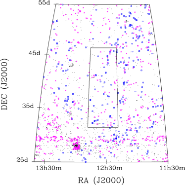
Figure 1: Surface distribution of galaxies in the CVn region. Every point in the plot corresponds to one detection in the CfA redshift survey catalogue (Huchra et al., 1999). From these, galaxies with the recession velocities $V_{LG}\leq 2000$ km s^-1 are presented with squares. Detections for which redshift measurement has not been provided are indicated by crosses. The area covered by the WSRT CVn survey has been marked with the combination of a continuous and a dotted line. The dotted line corresponds to the range in declinations for which two pointings per strip of constant declination have not been observed.

2.3 Data reduction

In total 1372 (useful) pointings were observed for this survey. Scripts were developed to automate the processing for this large number of pointings. The scripts were based on MIRIAD programmes (Sault et al., 1995) and programmes written by two of us (T.A.O. and K.K.). The data reduction process applied is described below.

The $uv$ data of each pointing were cross-calibrated and Hanning smoothed. The few first and last channels in the observed band were excluded because of their higher noise. The data were visually inspected and obviously bad data were flagged. To be able to see the H I  emission in the observed data, the continuum had to be subtracted. The continuum $uv$ data were created to first approximation by fitting a polynomial of second order to all available channels for each pointing, excluding the obvious line emission. After summing the continuum emission observed over the whole band into one plane, the data were Fourier transformed into ($\alpha$, $\delta$) continuum images using standard MIRIAD programmes. The final continuum image was created in an iterative process of cleaning and self-calibration of the continuum data. The line $uv$ data were obtained by copying the calibration coefficients and subtracting the modelled continuum emission from the observed data in the $uv$ domain.

The line $uv$ data were processed into ($\alpha$, $\delta$, $V$) line datacubes using the MIRIAD programme INVERT. The mosaicing mode of the observations produced data sampled very sparse in the $uv$ plane. In order to suppress large, shallow wings of the synthesised beam, a special weighting was applied to the $uv$ points. This weighting corresponds to natural weighting multiplied by radius in the $uv$ plane. The data were smoothed spatially by multiplying the $uv$ data with a Gaussian corresponding to a FWHM of 30 arcsec. From the first 9 $\times$ 12 hr of observations, 216 line datacubes each consisting of 115 channels (i.e. [$\alpha$, $\delta$] images) were obtained. The rest of the data were processed into 1156 line datacubes with 125 channels. Additional continuum subtraction was applied to all pointings by fitting the continuum with a polynomial of first order to the line datacubes excluding line emission, and subsequently subtracting it from them. The velocity spacing in the line datacubes produced is $\sim$ 16.5 km s^-1 and the velocity resolution after Hanning smoothing is $\sim$ 33 km s^-1. The size of the image in each of the channels is 512 $\times$ 512 pixels², with a pixel size of $8^{\prime\prime}\times 8^{\prime\prime}$. The typical spatial resolution of the datacubes produced is $\sim 30^{\prime\prime}\times 60^{\prime\prime}$.

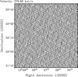
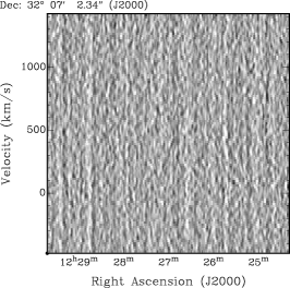
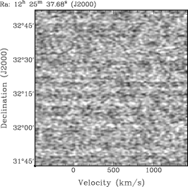
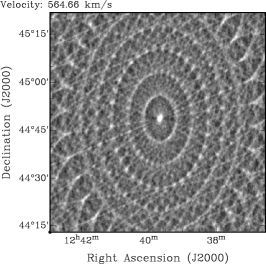
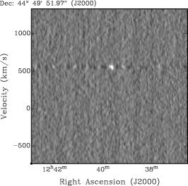
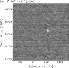
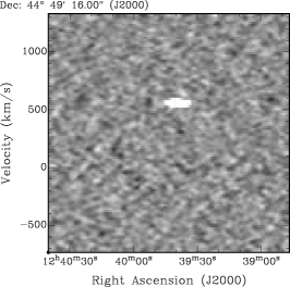
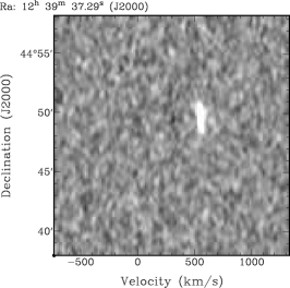
Figure 2: Examples of the various features in the line datacubes. The panels in the vertical direction are made by extracting one slice from the line datacubes in $\alpha-\delta$, $\alpha-V$ and $\delta-V$ planes, going from left to right respectively. Three uppermost panels show the appearance of the interference in the datacubes. The middle panels illustrate the grating rings formed around an H I source. The lowest panels show cuts through a final line datacube produced by combining nine of the line datacubes, created from the data observed for one pointing, and by cutting the central part of the combined datacube.

A known problem for detecting radio emission is man-made and natural interference. No good automated method exists for removing interference from the data, especially not from data observed in mosaicing method. In these kind of observations, marking the data as bad outside an interval of data values observed for an individual source (e.g. “sigma-clipping”) will not necessarily remove the data affected by interference. The scatter seen in the data can be caused both by the interference and by the observed source itself, because the $uv$ properties of a source can significantly change between the two consequent observations in the mosaic mode of that specific pointing. Therefore, all 1372 line datacubes were visually inspected. Datacubes are composed of 36 different $XX$, $YY$ scans and if interference occurred it was easily recognisable in the image domain, where the interference appeared as a strong narrow stripe. An example of the appearance of interference in the datacubes is presented in the three upper panels in Figure 2. Using the MIRIAD task CGCURS, stripes induced by the interference were marked and removed by flagging the $uv$ scan during which the interference occurred.

As a result of the sparse sampling in the $uv$ plane the sidelobe levels and grating rings around the strong H I sources preclude detecting faint H I  emission. Channels with H I  emission were CLEANed and RESTOREd with a Gaussian beam with a similar FWHM as the synthesised beam corresponding to the pointing. In the three middle panels in Figure 2 we show an example of grating rings produced around an H I source.

To exploit the observing strategy with overlapping pointings, line datacubes corresponding to the pointings with separation less or equal to 22 arcmin were combined into one datacube. Smaller datacubes of size 150 $\times$ 150 $\times$ 115 or 150 $\times$ 150 $\times$ 125 pixel³ in $\alpha\times\delta\times V$ directions respectively were cut out of the central part of each combined datacube, where the size of the third dimension depends on the observations. The $uv$ continuum subtraction worked well, leaving only minor residual effects in the image datacubes. These residual continuum features were removed using a simple linear baseline fit to the spectra in the datacube excluding the channels with H I emission. The small, combined line datacubes have been used for all of the further data analysis. In the following text they will be referred to as the full resolution datacubes. An example of the full resolution datacube is presented in the three lowest panels in Figure 2.

For each of the combined datacubes the synthesised beam of the central datacube used in the combining process was chosen as the beam of that datacube. Theoretically, all the $uv$ data observed in overlapping pointings could be used jointly to build a single large data cube, instead of applying the whole data reduction process on the individual pointings and then combining the cleaned and interference free line datacubes from the individual pointings. In practice, the first method would need much more computer time and computer memory, and at the moment it is not affordable for such a large data set as ours.

3 H I detections

3.1 Searching for detections

One of the most important aspects of analysing the observations is to define what constitutes a detection. In surveys, regardless of the observed wavelength, the common way is to consider a detection a real object if the measured flux, or part of it, of that particular object exceeds the noise by a certain factor (e.g. Wall & Jenkins, 2003).

The line datacubes, produced as described in the previous section, were smoothed both in the spatial and velocity domain in order to improve the detectability of extended objects with small signal to noise ratios. The datacubes were convolved with Gaussians with FWHMs such that the final spatial resolution of the produced smoothed datacubes was 1.5 and 2.0 times the original spatial resolution. In the velocity domain, cubes were Hanning smoothed by performing a weighted average of the fluxes over 5 and 7 neighbouring channels. Smoothing in the spatial and velocity domain was done separately.

To get a good insight in the statistical properties of the data, the mean and the rms values of datacubes were estimated for all of the 1372 line datacubes produced at the five different resolutions (the full resolution, 2 smoothed in the spatial domain and 2 smoothed in the velocity domain). The mean and the rms values of the individual datacubes were estimated from the pixels with absolute flux values below 5 times the preliminary rms value of the datacube. The preliminary rms was estimated using all of the pixels in the datacube. The binned distribution of the final rms values is presented in Figure 3, while the mean and the standard deviation of the measured rms values are presented in Table 2. For reference, we include in Table 2 the typical spatial and velocity resolution of the specific types of datacubes, as well as the limiting column density to detect an object with a profile width equal to the velocity resolution (third column in Table 2) at the 5-sigma (5 times the value in the forth column in Table 2) level. The mean noise value in the line datacubes with the full resolution is 0.86 mJy Beam^-1. For an object with a velocity width of 30 km s^-1 and an H I  mass of 10⁶ $M_{\odot}$ this noise limit would imply a maximum distance of 5.7 Mpc at which this object could be placed and still be detected in the survey at the 5-sigma level. In the same type of datacubes, the limiting column density to detect an object with a velocity width of 30 km s^-1 at the 5-sigma level is $7.9\times 10^{19}$ atoms cm^-2. This is only a crude estimate of the detection limit of the survey. A more precise estimate of the detection limit, based on the Monte Carlo simulations, will be presented in Subsection 4.2.

Figure 3: Statistics of the line datacubes. The panels show the histogram distributions of rms values measured for 1372 datacubes produced. In the first row results from the measurements in the datacubes with full resolution are presented. The second and the third rows contain the results for the datacubes smoothed in the spatial domain to the resolution 1.5 and 2 times the original resolution, respectively. The forth and the fifth rows present the statistics for the datacubes Hanning smoothed in the velocity domain averaging fluxes over 5 and 7 neighbouring channels, respectively.

	Resolution		rms		NHI
Datacube	spatial	velocity	mean	rms	[1020 $\times$
type	[arcsec2]	[km s-1]	[mJy Beam-1]	[mJy Beam-1]	atoms cm-2]
1.0	30 $\times$ 60	33	0.86	0.30	0.87
G1.5	45 $\times$ 90	33	1.33	3.01	0.60
G2.0	60 $\times$ 120	33	1.64	3.98	0.42
H5	30 $\times$ 60	82.5	0.67	0.28	1.70
H7	30 $\times$ 60	99	0.62	0.28	1.88

Table 2: Statistics of the 1372 line datacubes. The first row corresponds to the statistics of the full resolution datacubes. Statistics of the datacubes Gaussian smoothed in the spatial resolution by a factor 1.5 and 2 is given in the second and third row respectively. Statistics of the datacubes Hanning smoothed over 5 and 7 neighbouring velocity channels is presented in forth and fifth row respectively. See text for description of the columns.

The distribution of the observed pointings in this survey was designed in such a way that the noise in the combined datacubes is almost uniformly distributed. Still, the noise in some of the datacubes shows a gradient in the spatial domain along the declination axis. This is due to the fact that the final datacube is composed from observations typically collected during three different nights. The noise gradient reflects the difference in quality of the data collected during each single 12 hr period of observations caused by, for instance the loss of one of the 14 telescopes and the difference in the data flagging.

To overcome this problem, the noise in each pixel of the datacubes was modelled by averaging the standard deviations independently estimated in the spatial and velocity projections in the following way. First, the standard deviation of the flux values in the spectra at the position of every pixel in the spatial domain along the velocity was calculated. The standard deviation of the fluxes was calculated also for each of the channels in the datacube. For these calculations, pixels in the channels around zero velocity, where the Galactic emission can be very strong, were excluded. In the second iteration, in addition to the pixels in the region of Galactic emission, pixels with flux values larger or equal than 5 times noise from the first iteration were excluded also from the calculations. The “characteristic noise” of a pixel in a datacube was defined as the average value of the two standard deviations calculated in the second iteration for the plane and for the spectrum which both contained that pixel. This value will be referred to in the text as the noise ($\sigma$). The velocities with Galactic emission are in the range from approximately -50 km s^-1 to approximately 80 km s^-1  and from approximately -60 km s^-1  to approximately 85 km s^-1 for the datacubes produced from the poitings observed during the first 9 $\times$ 12 hr and during the remaining observations, respectively.

The next step was to inspect the line datacubes in order to detect the presence of H I  emission. All line datacubes were searched for pixels with an absolute flux value above a given limit expressed in multiples of the noise in each pixel. A procedure was developed to automate the process of searching for signal in the datacubes.

First, the procedure was used to find all pixels with absolute flux values above 5$\sigma$ in the datacubes of the 5 different resolutions. For a comparison of the detections, the search was also performed to detect pixels with absolute flux values above 4$\sigma$ for the line datacubes at the full resolution. The number of connected pixels with flux values above the given threshold (positive pixels in the remaining text) or below $-$1 times the given threshold (negative pixels) was counted. Pixels were classified as connected if they had at least one neighbouring pixel which passed the same searching criteria either in the spatial or velocity domain. Negative velocity regions were searched for galaxies, but the velocity range with Galactic emission (the same velocity intervals as in the noise calculations) was excluded from this search. The results of the process of the search for the regions of connected pixels are presented in Figure 4. The upper parts of all panels show the distribution of counts of the regions of connected pixels with positive flux values above the given threshold and negative flux values below $-$1 times the given threshold. The lower parts of all panels present the difference between the number counts of the regions of connected pixels with positive and negative flux values of a specific size over a range of sizes, where the size is expressed in pixels.

Figure 4: Distributions of counts of connected pixels with a certain positive and negative flux value revealed in the searching process. The upper parts of all panels show the distribution of counts of the regions of connected pixels with positive flux values above the given threshold (full line histograms) and negative flux values below $-$1 times the given threshold (dotted line histograms). The threshold is $5\sigma$ for the three upper ($a$, $b$, $c$) and the last two lower panels ($e$ and $f$) and $4\sigma$ for panel $d$. The vertical dashed line marks the position of the minimum number of connected pixels for a detection to be considered a real object. The lower parts of all panels present the difference between the number counts of the regions of connected pixels with positive and negative flux values of a specific size over a range of sizes, where the size is expressed in pixels. The panels $a$ and $d$ show the results of the searching process on datacubes with the full resolution. Panels $b$ and $c$ show the results of the searching process done on datacubes spatially smoothed with the Gaussians to the resolution 1.5 (panel $b$) and 2 (panel $c$) times the original spatial resolution. Results for the datacubes Hanning smoothed averaging over 5 neighbouring channels are presented in panel $e$ and for the datacubes Hanning smoothed averaging over 7 neighbouring channels are presented in panel $f$.

The thresholds to consider a detection as a real object were determined from the distributions of the number of connected positive and negative pixels for each of the six explored cases. The criteria were based on the expectation that the noise is distributed symmetrically. Detections were considered real objects if the number of connected positive pixels was larger than the largest number of connected negative pixels, which obviously corresponds to noise. For the datacubes with full resolution, a detection then is a real object if the number of connected pixels with flux values larger or equal than 5$\sigma$ is larger or equal than 10 pixels and the number of connected pixels with flux values larger or equal than 4$\sigma$ is larger or equal than 22 pixels. The typical beam size is approximately 32 pixels for the datacubes with full resolution. For the datacubes smoothed in the spatial resolution by a factor 1.5 and 2, a detection would be considered real if it contains larger or equal than 15 and larger or equal than 25 connected pixels with flux values larger or equal than 5$\sigma$ respectively. For the datacubes Hanning smoothed in velocity over 5 and 7 channels the number of connected pixels with flux values larger or equal than 5$\sigma$ had to be larger or equal than 12. From the distributions of all connected pixels with flux values in a certain interval, especially from the differences between the numbers of positive and negative connected pixels with the same number of pixels (Figure 4), it is obvious that there is no hidden distinct population of H I sources with flux values at the sub–noise levels. Such a population of missed objects would have been easily recognisable as a systematic offset of the difference between the positive and negative pixels with the same number of connected pixels towards positive values.

Applying the determined criteria, a unique catalogue of H I detections was created by the union of the 6 catalogues obtained by applying the specific searching criteria on the line datacubes of different type. In total, our search criteria reveal 70 H I detections which are considered real. All 70 detections were catalogued already in the datacubes with full resolution. No additional detection passed the “real object” criteria in the datacubes that were smoothed either in the spatial or velocity domain. There are no detections with lower column densities than the limiting column density which has already been achieved in the line datacubes at the full resolution.

There were 4 regions detected where the H I emission was very extended and the objects detected in these regions were of extremely irregular shape. For these cases the final decision what is an object was made by eye, after consulting previous observations available from the literature. These H I objects will be termed extended from here on. The extended objects are the objects with the WSRT–CVn id’s ranging from 63 and 68 including (with two objects with the WSRT-CVn id 67: 67A and 67B). More details on these and the rest of the objects will be given in the following text.

3.2 H I parametrisation

The H I parametrisation of the detected objects was carried out combining programmes developed for this survey and standard MIRIAD programmes. The cubes with full resolution in the spatial and velocity domains were used to determine the parameters of the H I detections.

The next task after the detecting of the objects was to determine the total flux of the object. Due to the uncertainty of the process, we have done this in two ways and taken the average of the two measurement as the total flux estimate.

The first method was to select the pixels which belong to an object (i.e. to mask all pixels with the signal). This was done in two steps. The first step was developed in order to recover the total flux of an object, and the second step was developed to recover the shape of an object. Starting from the pixel of the detection with the maximum flux value, the object was enlarged considering that all connected pixels with flux values larger than or equal to 3.5$\sigma$ belong to the object, using our definition of $\sigma$. The 3.5$\sigma$ limit was obtained as the optimal limiting flux value after testing various assumed limits to recover the total flux of an object in the INVERTED datacubes. For this test, we used the clean components of various objects inserted into the line datacubes, convolved with a cleaned beam of the datacube of the consideration previous to the insertion. The second step consisted of changing the shape of the masked pixels in each of the planes where the object was detected with significance above 3.5$\sigma$, to account for the fact that the detections in line datacubes are convolved with the beam of some finite size (which defines the spatial resolution element). First, to remove the detected pixels which are most probably only the noise, pixels with more than 3 neighbouring pixels which do not belong to the object (their flux values are smaller than 3.5$\sigma$) were deleted. After that, remaining pixels in the mask with at least one neighbouring pixel which does not belong to the object were marked as the border pixels. For each of the border pixels an area of a beam size centred on the border pixel was inspected. All pixels with positive flux values inside of the beam area studied were added to the detection. The total integrated flux ($S_{\rm int,c}$) of the detections was obtained by summing the flux in pixels determined to belong to the object in all channels and dividing this value by the beam area. The spatially integrated peak flux is simply the maximum value of the fluxes integrated in the individual channels (maximum in the spectrum, $S_{\rm peak,c}$). From now on, we will use the term integrated flux instead of the total integrated flux and the term integrated peak flux instead of the spatially integrated peak flux.

The size of the detected objects, which were not classified as extended objects, was estimated using the MIRIAD task IMFIT. A two-dimensional Gaussian was fitted to the H I  map, created by integrating the flux over the velocity channels contained in the masked pixels. When possible, we estimated the size of an object from the size of an ellipse fitted to a column density isophote of 1.25 $\times$ 10²⁰ atoms cm^-2. This isophotal level corresponds to a value of 1 $M_{\odot}$ pc^-2. For the small objects (WSRT–CVn 7, 10, 11, 12, 15, 19, 22, 25, 30, 31, 42, 43, 47 and 61) we used the FWHMs of the fitted Gaussian along the major and minor axis as a rough indicator of the angular size of an object. The FWHMs along major and minor axis and the positional angles obtained were deconvolved with the beam. The exceptions are detections with the WSRT–CVn id’s 7 and 47, which are too small to be deconvolved. For these two detections we present only the values of the FWHMs of a two-dimensional Gaussian convolved with a beam instead of their size. The last parameters will be used only as an indication of the inclination of these two objects. For the objects without a known counterpart in the literature, we use the position of the peak of the fitted Gaussian as the position of that particular object (the cross-correlation with literature detections is described in Subsection 5.1. Most of our detections are very small and the estimated H I sizes are very uncertain (see Table LABEL:prop2; for the objects with an estimated size comparable to or smaller than the beam size we use an $``<"$ sign to indicate that these sizes are probably just upper limits). However, they are usefull for a comparison with the sizes estimated from the optical measurements. We do not measure H I sizes of the extended objects, as the noise distribution in the datacubes of these objects is much more inhomogeneous and we are not able to apply the masking method reliably for these objects.

As the second method to estimate the total flux of an object the MIRIAD programme MBSPECT was used. The integrated H I spectrum of each detection was made, summing the flux in pixels contained in a box placed around the object and weighting the sum with the inverse value of the beam. The size of the box was estimated individually for each object based on the extent of the H I emission and always slightly bigger than the object itself, both in the spatial and in the velocity domain. For the extended objects, which have id’s from 63 till 68, this was the only method used to estimate these two parameters. We mark the integrated fluxes obtained with MBSPECT $S_{\rm int,MBSPECT}$ and the corresponding peak values of the integrated profiles $S_{\rm peak,MBSPECT}$. In Figure 5 the difference between integrated fluxes and peak fluxes measured using two different methods [(1)masking by defining pixels which belong to an object and (2) summing in a box using MBSPECT] is plotted. The difference is larger for the objects with lower values of integrated fluxes and integrated peak fluxes, where the influence of the noise in the flux values is relatively higher. Where possible, the average value from the two methods used to estimate integrated flux (S_int) and integrated peak flux (S_peak) will be used as the final estimate of these two parameters for the detected H I objects.

Figure 5: Comparison of the measured integrated flux (top) and integrated peak flux (bottom) values using two different methods for objects for which we have both measurements. Horizontal axis present the measurements based on the flux values in the pixels defined to belong to an object (masking). Vertical axis present the measurements using the MIRIAD task MBSPECT, defining the boxes around detections. The estimated errors for the presented parameters are described in Subsection 4.1.

The MIRIAD task MBSPECT was also used to parametrise the detections in velocity space. The widths of the profiles of the detections were measured at the 20% ($W_{20}^{obs}$) and 50% ($W_{50}^{obs}$) levels of the peak flux in the spectrum, using the methods of width maximisation and minimisation in MBSPECT. The maximisation procedure measures the line widths starting from the velocity limits given when specifying the box around a detection and moves inward till the percentage of the peak flux is reached. The minimisation procedure starts at velocity at which the profile has maximum and searches outward. The velocities at the centres of the four measured profile widths were also estimated. The radial velocity of a detection was estimated as the average of those four measured velocities. The velocities in the datacubes and spectra were calculated from the observed frequencies $\nu$ using the radio convention $V_{r}=c(1-\frac{\nu}{\nu_{0}})$. The estimated systemic velocity was recalculated to the value in the optical convention $V_{o}=c(\frac{\nu_{0}}{\nu}-1)$. The velocities in the optical convention were recalculated from the geocentric to the barycentric frame. In addition, they have been corrected for the motion of the Sun around the galactic centre and the motion of the Galaxy in the Local Group using the expression (Yahil et al., 1977)

$$V_{LG}=V_{o}+296\sin l\cos b-79\cos l\cos b-36\sin b$$ (1)

which is similar to the IAU convention. In this formulae $V_{LG}$ is the Local Group velocity and $l$ and $b$ are the galactic coordinates of the detection.

The profile widths measured from the data have been corrected for instrumental resolution. We used method given by Verheijen & Sancisi (2001) to correct for broadening of the global H I profiles due to a finite instrumental velocity resolution. Assuming a Gaussian line shape for the edge of the profile, the slopes of which are determined by the turbulent motion of the gas with a velocity dispersion of 10 km s^-1, this correction can be written in the form

$$W_{20}=W_{20}^{obs}-35.8\left[\sqrt{1+\left(\frac{R}{23.5}\right)^{2}}-1\right]$$ (2)

$$W_{50}=W_{50}^{obs}-23.5\left[\sqrt{1+\left(\frac{R}{23.5}\right)^{2}}-1\right].$$ (3)

for the widths at 20$\%$ and 50$\%$ of the peak flux respectively. The observed widths $W_{20}^{obs}$ and $W_{50}^{obs}$ were calculated by averaging the 20$\%$ and 50$\%$ level widths measured in the maximisation and minimisation procedure by MBSPECT. The instrumental velocity resolution $R$ expressed in km s^-1 was taken to be 33 km s^-1.

4 Parameter accuracy and completeness of the survey

We use an empirical approach to assess the accuracy of the measured parameters of the detections and the completeness of the survey. Our method is based on the inserting a large number of synthetic sources throughout the selected survey data. The major inputs to estimate the accuracy of the measured parameters are the recovered properties of the synthetic sources. The completeness of the survey is determined from the rate at which the synthetic sources could be recovered.

As a basis for the simulations, 10 line datacubes of full resolution were selected from the 1372 line datacubes produced in the whole survey. We refer to these datacubes as the basis datacubes. The datacubes selected were to our knowledge object free. Seven of the datacubes were selected from the central part of the area covered by the survey, while three of the datacubes were selected to be datacubes from the edges of the area covered by the survey; two of them are datacubes with one edge and one is a corner datacube with two edges.

The majority of the objects detected in the WSRT CVn survey are small H I objects, and the uncertainties and the completeness of these detections were the main focus for designing these simulations. The synthetic objects were created to resemble small H I objects, and therefore our simulations are not optimal for all possible types of H I objects. Five objects of different sizes in the spatial and velocity domains with different distributions of flux were created from the CLEAN components of H I  objects detected in the survey. Created objects are 2,3,4,5 and 6 channels wide. The profiles of the all synthetic objects were also of triangular shape. In each of the basis datacubes 10 objects were inserted and distributed quasi-randomly. Quasi-randomness in this context means that objects were inserted only in channels with positive velocities, as are all the real detections, and they were distributed in the datacube such as not to overlap with each other. It is possible is that some overlapping sources could be partially accreted dark galaxies which show up only as asymmetries in single detections. Our small sources are too small with respect to the beam size to study their shapes in detail. For the large sources, this remains an unexplored possibility.

The same synthetic objects were inserted at the same relative positions in all of the datacubes (same $x$, $y$ and $z$ of the three dimensional datacube), in order to emphasise the influence of the underlying noise in the datacube on the measured properties of inserted objects. Obviously, the noise distribution differs from datacube to datacube. Before inserting the objects into the datacube, their flux was rescaled and they were convolved with the beam of the line datacube in which they were going to be inserted. Each of the synthetic objects was inserted in two positions in the datacube, with two different flux values. In total ten runs were made, rescaling the maximum flux values two times for the 5 different model-objects in each of the datacubes. In the first run of simulations, the maximum value of different model-objects were fixed at 1.0 and 3.0 mJy and in each of the following 9 simulation runs the peak value was increased by 0.2 mJy. These flux values were chosen in such a way to ensure that there is a fraction of synthetic sources which will not be detected. In total 1000 different objects were inserted in 10 different datacubes.

The datacubes with inserted synthetic objects were then searched for these synthetic sources in a manner identical to the searching process used in the WSRT CVn survey, as described in Subsection 3.1. Detections which satisfied the criteria for real objects were parametrised the same way as the real detections, described in Subsection 3.2. The simulation described above was used to estimate the uncertainties of the measured H I parameters and the completeness of the WSRT CVn survey in the following two subsections, respectively.

One of the shortcomings of our simulations is that all synthetic sources have profile widths of triangular shape. Zwaan et al. (2004) estimated parameter uncertainties and completeness of HIPASS (a single dish survey) using synthetic sources of Gaussian (e.g. triangular), double-horned and flat-topped profile shapes. Within the errors, the completeness of the survey is the same for all types of profiles. Zwaan et al. (2004) did not discuss the uncertainties in the measured parameters on the profile shape.

4.1 Parameter uncertainties

The uncertainties of the H I  parameters can be estimated from a comparison of the assigned and measured properties of the synthetic objects revealed in the simulated datacubes. In the simulations described above, 794 of the inserted 1000 synthetic sources were recovered using the searching criteria defined for the datacubes with the full resolution: at least 22 connected pixels with flux values larger or equal than 4$\sigma$. Parametrisation of the sources detected in the simulation was carried out and the distributions of differences between the real and the parameterised properties of the population of synthetic objects revealed in the simulation are presented in Figure 6.

From the distributions of differences, the uncertainties of S_int, S_peak  and profile widths measured at 50$\%$ and 20$\%$ of the line maximum were calculated as the standard deviation in the corresponding distributions. The uncertainties of the measured integrated fluxes in the WSRT CVn survey are $\sigma=0.421$ Jy km s^-1 for the case of the flux summed inside of the defined contour, $\sigma=0.242$ Jy km s^-1 for the flux inside of a box around a detection, while $\sigma=0.240$ Jy km s^-1 for the flux of an object calculated as the average value measured from the two techniques used. For the integrated peak fluxes, uncertainties are $\sigma=8.8$ mJy, $\sigma=3.7$ mJy and $\sigma=4.7$ mJy for the three methods used, given in the same order as the S_int  uncertainties above. Uncertainties for the profile widths (as observed) are $\sigma=5.1$ km s^-1 and $\sigma=8.4$ km s^-1 for the profile widths measured at 50$\%$ and 20$\%$, respectively.

The detectability of a 21-cm signal depends not only on the flux, but also on how this flux is distributed over the velocity width of the object of consideration. There is probably a more complicated dependence of the uncertainties of the estimated H I  parameters on the intrinsic properties of an object. Given the relatively small number of detections in the WSRT CVn survey, we neglect such a dependence in our results. We only demonstrate the existence of the additional dependence of measured S_int values on the values of S_int, S_peak  and profile width. The results are presented in Figure 7. Here, the difference $\Delta$S_int corresponds to the difference between the value of the integrated flux inserted and the integrated flux measured, calculated as the average value of the integrated flux obtained by using our programmes – defining a mask around a detection, and the integrated flux obtained by using the MIRIAD task MBSPECT – defining a box around a detection. The uncertainty of S_int is 0.130 Jy km s^-1 in the range of true values S_int $\leq 0.5$ Jy km s^-1  (continuous line in the left panel in Figure 7), 0.188 Jy km s^-1 for $0.5<$ S_int $\leq 1$ Jy km s^-1 (short dashed line), 0.280 Jy km s^-1 for $1<$ S_int $\leq 2$ Jy km s^-1  (dotted line) and 0.278 Jy km s^-1 for S_int $>2$ Jy km s^-1 (long dashed line). To test the dependence of $\Delta$S_int on the S_peak value of the inserted detection, we split the S_peak values in the four arbitrary intervals: S_peak $\leq 0.01$ Jy (continous line), $0.01<$ S_peak $\leq 0.02$ Jy (short dashed line), $0.02<$ S_peak  $\leq 0.04$ Jy (dotted line) and S_peak $>0.04$ Jy (long dashed line). The uncertainties are 0.134 Jy, 0.168 Jy, 0.278 Jy and 0.265 Jy for the given intervals, respectively. Finally, we divided $\Delta$S_int  values in the three intervals depending on the $W_{20}^{obs}$ of the object. The uncertainty in S_int for the objects with: $W_{20}^{obs}\leq 45$ km s^-1 (continuous line) is 0.156 Jy km s^-1, $45<W_{20}^{obs}\leq 60$ km s^-1 (short dashed line) is 0.091 Jy km s^-1 and $W_{20}^{obs}>$ 60 km s^-1 (dotted line) is 0.285 Jy km s^-1.

Figure 6: Comparison between inserted and measured parameters. The first two panels show the difference between the values of inserted parameters and parameters measured by forming a mask around a detection (full line histogram) and parameters measured with MBSPECT (dashed line histogram). The first panel shows the difference distribution for integrated flux values. The second panel shows the distribution of differences in integrated peak flux values. Third panel shows the difference between the inserted profile widths and recovered profile widths at 20% of the maximum in a spectrum (full line histogram) and at 50% of the maximum in a spectrum (dashed line histogram), measured with MBSPECT.

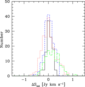
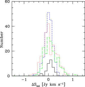
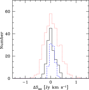
Figure 7: Distributions of $\Delta$S_int, differences between the inserted integrated fluxes and detected integrated fluxes, as a function of inserted S_int, S_peak and profile width. The detected S_int values are calculated as the average value of the integrated flux calculated by defining a mask around a detection and the integrated flux obtained by using the MIRIAD task MBSPECT, defining a box around a detection. In the left panel the continuous (black) line corresponds the the distribution of $\Delta$S_int for S_int $\leq 0.5$ Jy km s^-1, the short dashed line (blue) is the same type of distribution for $0.5<$ S_int  $\leq 1$ Jy km s^-1, dotted (red) line for $1<$ S_int $\leq 2$ Jy km s^-1 and long dashed (green) line for S_int $>2$ Jy km s^-1. Middle panel shows the distribution of $\Delta$S_int  as a function of S_peak. The continuous (black) line is for S_peak $\leq 0.01$ Jy, the short dashed (blue) line for $0.01<$ S_peak $\leq 0.02$ Jy, dotted (red) line is for $0.02<$ S_peak $\leq 0.04$ Jy and long dashed (green) line is for S_peak $>0.04$ Jy. The right panel shows the distribution of $\Delta$S_int as a function of $W_{20}$ for the range of: $W_{20}^{obs}\leq 45$ km s^-1 – continuous (black) line, $45<W_{20}^{obs}\leq 60$ km s^-1  – short dashed (blue) line and $W_{20}^{obs}>60$ km s^-1 – dotted (red) line.

4.2 Completeness

Completeness of the survey is the fraction of galaxies detected in a given volume down to the limiting sensitivity. The completeness of the blind WSRT CVn survey is addressed using the Monte Carlo simulations described. It is defined here as the ratio of the number of synthetic objects detected in the simulations and the number of synthetic objects inserted in the simulation.

The completeness of the survey is estimated as a function of S_int and S_peak values. To take into account all possible sources which would be detected in the real survey, datacubes with the inserted synthetic sources were smoothed in the spatial and velocity domain. The smoothing was identical to the smoothing of the real datacubes. The smoothed datacubes were searched in all resolutions applying the criteria as defined in Subsection 3.1. This resulted in the completeness corrections shown in Figure 8 that were later applied in deriving the H I mass function.

The fraction of datacubes with one or two edges used in the simulations was much larger than the fraction of datacubes with edges in the real survey. To account for this, the completeness of the survey was estimated for each type of the datacube independently. The reason for including the datacubes with edges and testing them separately was that the noise distribution in the edge cubes is much more inhomogeneous. The completeness of the whole WSRT CVn survey was calculated weighting the number of detected objects with the relative abundance of the type of datacubes (in the survey) in which these objects were detected. The weighted completeness is considered to be the best estimate of the completeness of the whole survey. It is presented with the continuous line in Figure 8. From the simulations carried out, it follows that the WSRT CVn survey is complete, at least in a statistical sense, for objects with approximately S_int $>0.9$ Jy km s^-1 and S_peak $>0.0175$ Jy. From 70 objects detected in the WSRT CVn survey, 12 of them have S_int values in the range for which the survey is incomplete. For only 2 detections the incompleteness is larger than 50%. The minimum integrated flux of an object has to be 0.2 Jy km s^-1 (centre of the first bin with a non-zero completeness) in order to be detected in the WSRT CVn survey.

Figure 8: Completeness of the WSRT CVn survey. Circles represents the fraction of objects detected in the datacubes within the survey, without an edge. Squares correspond to the fraction of detected objects residing in the datacubes with one edge and triangles represent the fraction of objects detected in the datacubes with two edges. The continuous line connects the bins with a fraction of detected objects weighted with the relative abundance of a type of the datacube in which the detection resides. The long dashed line connects fractions of all objects detected in the simulation regardless of the type of the datacube in which the detection was inserted. The short dashed horizontal line represents the line for which the survey is complete. The errors are estimated from the binomial statistics. For clarity, the errors are presented only for the completeness based on all datacubes without weighting for the datacube type, and they are offset along x-axis.

5 Properties of the H I detections

5.1 Comparison of the detections with previous observations

The cross–correlation of the objects detected in the WSRT CVn blind survey with known objects was conducted using the NASA/IPAC extragalactic Database (NED). Both, positional and velocity information, if available, was used to identify a counterpart of each of the detected H I  sources. In addition, the Lyon/Meudon Extragalactic Database (HYPERLEDA) was used and the second generation Digital Sky Survey (DSS) images, centred on the position of the WSRT CVn detections, were visually inspected. We inspected also the SDSS images. We used the SDSS object identification and their redshift, if obtained, only in combination with the visual inspections of the images of cross-correlated galaxies, or parts of them, because of the not yet fully resolved problem with deblending of the extended sources (e.g. West 2005, http://www.sdss.org/dr7/products/catalogs/index.html$\#$cav$\_$lowlat).

In total 67 objects detected in the WSRT CVn survey were identified as galaxies previously detected in one of the optical wavebands. The cross-correlation is based on both the positional and velocity information for 58 objects. Objects WSRT–CVn–67A and WSRT–CVn–67B were cross-identified with two galaxies based on position and redshift information in the literature: NGC4490 and NGC4485, respectively. Using our data, we were not able to separate the 21-cm emission detected around WSRT–CVn–67A and WSRT–CVn–67B into two individual detections. Object WSRT–CVn–34 (UGCA290) looks like an interacting binary system, addressed as such in some references. We consider it as one object, a patchy dwarf galaxy, based on the resolved stellar photometry carried out by Makarova et al. (1998).

For the remaining 9 H I detections (WSRT CVn 8, 13, 17, 19, 25, 30, 31, 47 and 55) the cross-correlation with the previous detections is based solely on the positional information of the assigned optical counterparts. Given that these galaxies are best visible in blue light and $\sim$ 10-20 arcsec in size, it is most probable, even without knowing their redshifts, that they are the optical counterparts of the H I  detections. Close to the position of two additional H I detections, galaxies are visible in both DSS and SDSS images. One of these galaxies (which overlaps WSRT CVn 42) is detected in the SDSS splitted into multiple detections (in the currently last available SDSS data release 7), therefore there does not exist a uniquely previusly identified galaxy for this H I object. Two blue galaxies are detected in the area of the projected H I of WSRT CVn 40 (see Appendix A). One of these galaxies has the SDSS measured redshift $z=0.029$, which completely disqualifies it as a possible contributor to the detected H I. We cross-correlate therefore WSRT CVn 40 with the other galaxy. This galaxy is not detected by the SDSS pipeline, probably due to its proximity to a star.

An important question related to the cross-correlation of objects when using only positions and some properties of galaxies is what is the probability that this H I-optical pair is only a chance projection. The geometric probability $P$ that a galaxy of magnitude $m$ and at angular distance $\theta$ from the studied galaxies is only a chance projection (neglecting the correlation properties of galaxies) is given by (e.g. Wu & Keel, 1998)

$$P(\theta,m)=1-\exp(-\pi\rho(m)\theta^{2})$$ (4)

where $\rho(m)$ is the surface number density of galaxies brighter than $m$. We obtained the surface number density of galaxies from the SDSS database by counting the number of galaxies within 11 randomly placed pointings of a radius 30 arcmin in the WSRT CVn survey region. Properties of galaxies were selected to resemble the properties of the secure host galaxies of the faint H I detections. Roughly, we have taken $16<r<20$ mag and $0.2<g-r<0.6$ (see Chapter 5 in Kovač, 2007). We measured the density of galaxies with these properties to be about 52 per a pointing, leading to a probability that the cross-correlated opticaly identified galaxy is only a chance projection of 0.056 or 0.00014, if the optical detection is at a distance of 1 or 0.5 arcmin, respectively from the H I detection. From the inspection of the images of the H I overlayed on the top of the optical counterpart, it is clear that the projected distances between the optical detection and the maximum in the H I surface density are less than 1 arcmin. We conclude that also our cross-correlations without the known distances of the optically detected galaxies are pretty secure. Moreover, our measurements provide first measurements of distances to these galaxies.

Finally, based on the inspection of the DSS and SDSS images, there was one object detected in H I without an optical counterpart (WSRT–CVn–61). This object is found a few arcmin away and within $\sim 110$ km s^-1  from NGC 4288 (WSRT–CVn–62). This object has already been detected in H I by Wilcots et al. (1996) in H I  observations of a sample of five barred Magellanic spiral type galaxies. Interestingly, Wilcots et al. (1996) detected similar H I  clouds, without an obvious optical counterpart on the Digital Sky Survey images, and with the H I  mass $\sim$ 10⁷ $M_{\odot}$ in four out of five galaxies in their sample. In our data, WSRT–CVn–61 is barely resolved (see Appendix A), but clearly distinguished from NGC 4288 in the velocity. It has a single-peaked global H I profile, consistent with a very weak rotation (W${}_{50}\sim$ 20 km s^-1).

Potentially, detecting a dark object is very interesting in the context of this paper. We have carried out a follow-up optical observations in the field of NGC 4288, using the Wide Field Camera on the Isaac Newton 2.5 meter telescope, La Palma, Canary Islands. The observations did not reveal any sign of the stellar light nearby the position of WSRT–CVn–61 down to the surface brightness limit of 26.3 mag arcsec^-2 in $R$ and 27.4 mag arcsec^-2 in $B$ (Kovač, 2007, Chapter 5). The observations will be presented in more details in a future paper. To conclude, the nature of WSRT–CVn–61 is not entirely clear, but given its proximity to NGC 4288, it is likely a very LSB companion to this galaxy. We treat it as a separate object.

The homogenised H I  data (HOMHI) catalogue (Paturel et al., 2003) represents a compilation of H I  detections from 611 papers. This catalogue was used to inspect the whole volume covered by this survey for previous H I detections. According to the HOMHI catalogue there are 47 objects which have been observed in the 21-cm line inside the volume of the WSRT CVn survey and 4 objects are at the edges of the observed region (objects with WSRT–CVn indexes 1, 2, 60 and 62). Of the 47 HOMHI detections inside the survey volume, 44 can be cross-correlated uniquely with the WSRT CVn detections using their position on the sky and their heliocentric velocities. One of the detections of the WSRT CVn survey (WSRT–CVn–23) is cross-correlated with two objects in the HOMHI catalogue. These two HOMHI detections have the same heliocentric velocity, and their positions differ by 0.015 deg and 0.14 deg in right ascension and declination, respectively. Their profile widths are identical and their S_int values are almost the same. From tracing these detections back in the literature it follows that their names have been confused; there is only one object detected with the given H I properties and velocity.

One of the HOMHI detections does not have a counterpart in the WSRT CVn survey. That is MAPS$\_$NGP O$\_$218$\_$0783987, with heliocentric velocity 636 km s^-1. Huchtmeier et al. (2000) measured S_int = 0.66 Jy km s^-1, S_peak = 0.026 $\pm$ 0.0046 Jy, $W_{50}$ = 27 km s^-1 and $W_{20}$ = 34 km s^-1 for this object, using the single dish 100-m radio telescope at Effelsberg. The WSRT CVn survey is slightly incomplete ($C>90\%$) for the S_int  value and complete for the S_peak  value of this object. We carefully examined the datacube from the WSRT CVn survey produced at the position of MAPS$\_$NGP O$\_$218$\_$0783987. There is no sign of the 21-cm emission at that position in our data. Based on the cross-correlation with the previous observations, all detections from the WSRT CVn survey are real. We are inclined to believe that the detection in the Huchtmeier et al. (2000) sample is not real, but is, perhaps interference.

There is no entry in the HOMHI catalogue for objects WSRT–CVn–9 and WSRT–CVn-61. HYPERLEDA, however, provides H I data for WSRT–CVn–9. For a comparison with the literature, we used the measurement from Wilcots et al. (1996) for object WSRT–CVn-61. Object WSRT–CVn–7 has been listed in the HOMHI catalogue, but without a measurement of integrated flux. We obtained the S_int  value for WSRT–CVn–7 from Matthews & van Driel (2000). This S_int value has been corrected for the finite size of the Nançay telescope beam. In total, from 70 detected H I sources in the WSRT CVn survey, 19 have been detected for the first time in the 21-cm emission line in this survey.

Figure 9: Comparison of the WSRT CVn S_int  values with literature measurements. For WSRT–CVn–7 and WSRT–CVn-61 S_int, literature measurements come from Matthews & van Driel (2000) and Wilcots et al. (1996) respectively. In the top panel, literature values of integrated fluxes obtained from HYPERLEDA have been used. In the bottom panel integrated fluxes published in RC3 have been used. The integrated flux values of objects for which there is no previous H I measurement in the literature has been indicated with an “x” symbol. S_int  values of detections without RC3 measurements, but for which the S_int value in the HOMHI catalogue is available, have been indicated in the bottom panel with an “+” symbol. We plot the errors only for our measurements.

In Figure 9, the comparison of S_int values measured in the WSRT CVn survey and S_int values available from the literature is presented. For objects with the WSRT–CVn indexes 7 and 61 we use the values from the references given above. For the comparison presented in the top panel in Figure 9, we used the S_int values retrieved from HYPERLEDA for the rest of the objects. It is obvious that the HYPERLEDA integrated fluxes are systematically smaller than the WSRT CVn integrated fluxes for approximately S_int  $>10$ Jy km s^-1. The S_int values in HYPERLEDA come from the HOMHI catalogue (with the exception of object WSRT–CVn–9) and the majority of them have been measured with a single dish telescope. We have not traced back in the literature the references for the individual detections from the HOMHI catalogue. Instead, we collected S_int values for the WSRT CVn detections from the earlier RC3 catalogue (de Vaucouleurs et al., 1991). These two catalogues (HOMHI and RC3) are not independent. The comparison between the integrated flux values measured in the WSRT CVn survey and the literature S_int  values collected from the RC3 catalogue, and for the objects with the id’s 7 and 61 from the individual papers, is presented in the bottom panel in Figure 9. The RC3 catalogue contains S_int values for fewer objects detected in the WSRT CVn survey than the HOMHI catalogue. Still, most of the objects with S_int  values above 10 Jy km s^-1  are present in both catalogues considered. There is no systematic difference between the WSRT CVn integrated fluxes and the RC3 integrated fluxes. It is possible, that the systematic offset seen between our values of the integrated fluxes and those in the HOMHI catalogue is due to the corrections applied in the homogenisation process of the H I data used to create the H I parameters provided in the HOMHI catalogue. This difference can arise also from the distribution of H I in a galaxy. We use the interferometric data and we are restricted to the flux measurements in the galaxies. If a galaxy has a lot of outlying H I, we are not sensitive to include it, while the single dish observation picks it up. Given that our measurements agree with the RC3, we use the RC3 measurements of S_int, heliocentric velocity, $W_{50}$ and $W_{20}$ for objects WSRT–CVn–67A and WSRT–CVn-67B, for which we can not properly measure the H I properties from the WSRT CVn survey data.

5.2 Distributions of H I properties of the detections

The various distributions of the measured parameters of objects detected in H I  in this survey can be used to examine the basic properties of the detected sample. Histograms of the distributions with radial velocity, integrated flux, peak flux and profile width at the 50$\%$ level of the maximum flux in the spectra are shown in Figure 10.

Figure 10: Distributions of estimated H I parameters. Histograms show the number distribution of the WSRT CVn detections in bins of $cz$ (top–left), S_int  (top–right), S_peak  (bottom-left) and $W_{50}$ (bottom-right).

The redshift distribution of the detected objects is presented in the top left histogram. A fraction of 29$\%$ of all detections fall in a 100 km s^-1  wide interval with velocities $525\leq cz\leq 625$ km s^-1. This peak coincides with the peak of the CVnII cloud (Tully & Fisher, 1987). The peak of the CVnI cloud is at $\sim$ 300 km s^-1 (Tully & Fisher, 1987), clearly identifiable in the histogram of observed redshifts.

The distribution of measured S_int values is shown in the top right panel of Figure 10. The detections with values S_int $\geq 80$ Jy km s^-1, 6 in total, are excluded from the plot. The distribution of S_peak  values is presented in the bottom left panel of Figure 10. Most of the objects detected in the WSRT CVn survey have the small S_int and S_peak values measured. For example, a fraction of $63\%$ of the detected objects have S_int $\leq 10$ Jy km s^-1, while 72$\%$ of the detections with available S_peak measurements, have $S_{\rm{peak}}\leq 0.2$ Jy.

The last panel, bottom right in Figure 10, corresponds to the distribution of the profile widths at the 50$\%$ level of the maximum flux in the spectra of the detected objects, $W_{50}$ (corrected for the instrumental effects). This distribution has a prominent peak around $W_{50}\sim 35$ km s^-1. 86$\%$ of the detected H I objects have $W_{50}\leq 130$ km s^-1 and can be considered as a candidate population of dwarf galaxies (Duc et al. 1999 found that 75$\%$ of galaxies selected by the same profile width criteria are genuine dwarf galaxies). However, the observed profile widths are affected by the inclination of a galaxy, and we discuss this issue in more detail in Subsection 5.3.

Figure 11: Bi–variate distributions of observed parameters: S_int, S_peak, $W_{50}$, $cz$ and H I size. The objects detected for the first time in the 21–cm emission line in the WSRT CVn survey have been presented with open symbols; the remaining objects are marked with filled symbols. In the plots in the bottom-row, objects for which size is estimated from the isophote at a column density level of 1.25 $\times$ 10²⁰ atoms cm^-2 are marked with squares; if their size is estimated from a Gaussian fitted to the H I distribution they are marked with triangles. In the plot in the middle–left panel lines of a constant H I mass are shown (dotted lines). The H I mass of a detection (in $M_{\odot}$) has been calculated assuming an optically thin approximation, M_HI = 2.356 $\times$ 10⁵ d² S_int, for S_int expressed in Jy km s^-1 and $d$ being the distance to an object in Mpc. We assumed $d=cz/H_{0}$ and we used $H_{0}$ = 70 $\mbox{\mbox{km s${}^{-1}$}\ Mpc${}^{-2}$}.$ The lines of constant H I mass in $M_{\odot}$ are presented with a logarithmic step of 1. The horizontal continuous lines represent the maximum recession velocity up to which an object of a certain H I mass can be detected in the WSRT CVn survey. We used the same assumption about the distance to an object as described above. The minimum detectable integrated flux in the WSRT CVn survey is 0.2 Jy km s^-1, obtained from the calculations of the completeness of the survey. However, we are complete only for S_int measurements above 0.9 Jy km s^-1.

The bivariate distributions of velocity, profile width, peak flux, integrated flux and size are shown in Figure 11. Objects detected for the first time in H I in this survey are marked with open symbols. It is clearly visible that the newly detected H I objects have small integrated fluxes and integrated peak fluxes, small profile widths and small physical sizes.

The log-log plot of S_peak  vs. S_int demonstrates the simple property that H I  detections with larger integrated fluxes have higher integrated peak fluxes and vice versa. It is interesting that this relation holds for the detections over the whole range of observed integrated fluxes and integrated peak fluxes. The bivariate distributions of W₅₀ vs. S_int or S_peak show that there are no galaxies with large W₅₀ with small integrated fluxes and low integrated peak fluxes in the volume probed. Objects with small integrated fluxes spread over large profile widths (if they exist) would be very difficult to detect. Similarly, low S_peak galaxies with large line widths cannot be detected, because the flux is in the noise. Smoothing in the velocity domain increases the sensitivity to this type of objects. However, smoothing the datacubes in the WSRT CVn survey in the velocity domain, did not reveal any new detections.

The distributions of measured H I parameters with redshift ($cz$), show a segregation of detections in two groups, reflecting the positions of the CVnI and CVnII clouds in redshift space. In the redshift distributions of S_int  and S_peak there appears to be an absence of detections with small S_int  (and small S_peak) at low $cz$, also in that part of parameter space for which the survey is complete. The survey by itself does not have any selection effects which would bias it against the detection of objects in the nearby Universe with small integrated fluxes. As already discussed in Subsection 5.1, comparing our detections to previous H I observations reveals that there are no H I objects with $cz\leq$ 400 km s^-1 which have been missed in the WSRT CVn survey. Therefore, the absence of an H I  population with S_int $\leq$ 6 Jy km s^-1 (or S_peak $\leq$ 0.1 Jy) is real. However, taking a flat H I mass function and the number of detected objects in the higher mass bin 10⁷-10⁸ $M_{\odot}$(5), one would expect $5\pm\sqrt{5}$ objects in the 10⁶-10⁷ $M_{\odot}$bin, which is not too inconsistent. Moreover, the volume of the survey region limited with $85<cz<322.5$ km s^-1  is less than 1 h${}_{70}^{-3}$Mpc³. The observed redshift distributions of S_int  and S_peak probably reflect just a peculiarity of the CVnI group.

In addition, we present the bivariate distributions of $cz$, S_int and $W_{50}$ as a function of size of those objects for which the size was estimated. We used the average value of the major and minor axis estimated at a column density level of 1.25 $\times$ 10²⁰ atoms cm^-2, or only the FWHMs along the major and minor axis of a Gaussian fitted to the small detections. To express the size in kpc instead of arcsec we have adopted distances $d$ to the objects calculated from $d=cz/H_{0}$ using $H_{0}=70$ km s^-1 Mpc^-2.

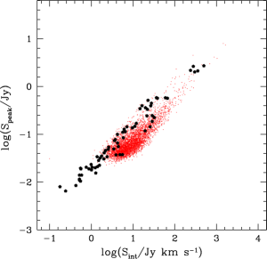
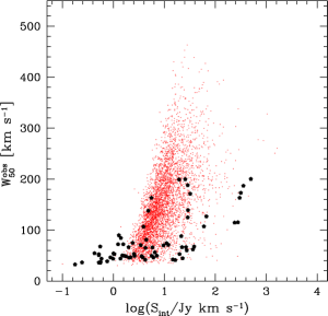
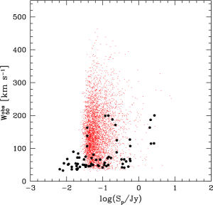
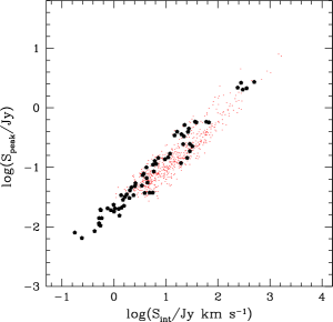
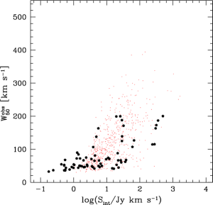
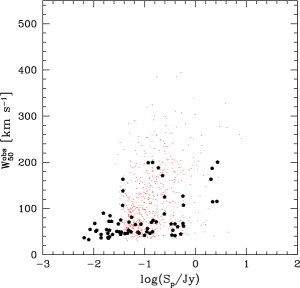
Figure 12: Comparison with the HIPASS detections. Small dots represent the HIPASS measurements. Big filled pentagons correspond to the WSRT CVn measurements. Profile widths have not been corrected for instrumental resolution, except for the objects WSRT–CVn–67A and WSRT–CVn-67B for which the literature values of profile widths, already corrected for instrumental broadening, have been used in the middle panels. The properties of the WSRT CVn detections are compared with the properties of the all HIPASS detections in three upper panels and with the properties of a subset of the HIPASS detections limited with $V_{LG}\leq$ 1400 km s^-1 in three lower panels, respectively. We detect very few big objects, i.e. galaxies with broad profiles and low S_peak but large S_int (when integrated over velocity). At larger distances these start to dominate the sample. The comparison with the near galaxies in HIPASS in the bottom left panel clearly underlines this.

To get an idea which part of the space of H I parameters is explored in the WSRT CVn survey, the measured properties of objects detected in this survey are compared to the properties of objects detected in the southern $\delta<2^{0}$ part of the H I Parkes All Sky Survey (HIPASS, Barnes et al.,, 2001; Meyer et al.,, 2004). Bivariate distributions of S_int, S_peak  and W${}_{50}^{obs}$ are plotted in Figure 12. Values of $W_{50}^{obs}$ used in the comparison have not been corrected for instrumental resolution, with the exception of the objects with WSRT-CVn id’s 67A and 67B, for which the $W_{50}^{res}$ values obtained from the literature have been already corrected for the finite spatial resolution of the H I observations. The beam size of the HIPASS survey is 15.5 arcmin. It can be expected that due to the large size of the beam some of the HIPASS detections correspond to multiple objects. From the comparison of integrated fluxes and integrated peak fluxes of the detections from the two blind H I surveys it follows that the WSRT CVn survey reveals H I objects with S_int and S_peak about 10 times smaller than the smallest HIPASS detections. This confirms our ability to detect objects which are faint in H I. The relative number of small mass objects (objects with small velocity widths, see in Subsection 5.3 discussion on the effect of the inclination) in the WSRT CVn survey is much larger when compared to the relative amount of low mass systems detected in HIPASS. On the other hand, large (massive) galaxies have not been detected in the volume covered by the WSRT CVn survey. All detections in the WSRT CVn survey have W${}_{50}^{obs}\leq 200$ km s^-1, while the detection with the broadest profile in the HIPASS has W${}_{50}^{obs}\sim 460$ km s^-1. This is expected for the volume covered by the WSRT CVn survey because the H IMF is a Schechter function with a flat faint end slope. The WSRT CVn survey samples with high sensitivity a specific region of the sky up to a distance corresponding to $cz\sim 1330$ km s^-1, known to be populated by small, gas-rich galaxies at small distances. The HIPASS survey goes much deeper, up to $cz\sim 13000$ km s^-1, and covers a variety of environments. Therefore, for an easier comparison, we include the same type of plots for the subset of HIPASS detections limited with $V_{LG}\leq$ 1400 km s^-1. Here, we mainly want to point out that the WSRT CVn survey has a much lower flux limit S_int than HIPASS.

5.3 Effects of the inclination

In the following section we discuss the importance of the inclination of the objects on the results presented. We use the sizes of the objects measured from the H I images, assuming intrinsically circular simmetry, to obtain the inclination $i$ of an object according to $\cos i=(b/a)$. Because some objects are very small or have patchy H I  distributions the derived inclinations are only indicative (i.e. they are very uncertain). However, our main goal here is to discuss the influence of the inclination of galaxies to the results presented so far: to the measured velocity widths and to understand if we have missed some H I objects because of inclination effects. From the $b/a$ distribution (see discussion below) it appears that the errors in the measured inclinations are random (due to the noise in the data) and not systematic. We believe that for our purpose the inclinations measured from the H I data should be sufficient.

Figure 13: Histogram of $b/a$ ratios for 63 objects detected in the WSRT CVn survey. $a$ and $b$ values are obtained from the H I data.

As described in Subsection 3.2, we estimated the H I sizes for 61 objects detected in the survey. For 2 additional objects we used the FWHM of a fitted Gaussian, not deconvolved for the synthesised beam as these objects were too small. The histogram of the H I  axis ratios $b/a$ of the detections is presented in Figure 13. The distribution of $b/a$ ratios of a sample of infitely thin and round discs projected randomly on the sky will be flat (Hubble, 1926). It is clear, that the distribution of $b/a$ values for the galaxies in this survey is not flat, also when considering Poisson errors in the $b/a$ bins, and we need to understand why this is the case.

An important question is if there is a population of H I galaxies which has been missed in the survey due to their specific inclination. Could the WSRT CVn survey miss galaxies with both small and large $b/a$ ratios? Apart from the errors in estimating the H I diameters of the detected objects, there are two additional effects which can cause the observed $b/a$ distribution. First, $b/a$ can not equal 1 if disks are not circular. For example, the average face-on system in the complete sample of Sb-Sc galaxies selected from ESO-LV survey has $b/a\sim 0.7$ (Valentijn, 1994). Second, if a galaxy has a finite thickness $z$, it means that there is a minimum $b/a$ value, and one should see an excess of galaxies at that value (equal to $z/a$) and a deficit below that value. The H I disks are of finite thickness and the lack of detections with low $b/a$ ratios probably reflects this effect. So qualitatively, we can explain both deficits in the histogram of $b/a$ ratios of the H I distributions. The conclusion then is that there is no population of H I objects with large and small $b/a$ ratios which has been systematically missed in the survey.

Figure 14: Distribution of the inclination corrected $W_{50,i}$ values with recession velocity. The open symbols are detections with H I measurements obtained for the first time in this survey. The filled symbols correspond to the detections with existing H I data in the literature.

Quantitatively, this conclusion no systematically missed detections) is confirmed by the previous H I observations carried out in the volume probed by the WSRT CVn survey. The CVnI cloud is nearby and a large number of observations has been carried out in this region, sometimes with much longer integration times. However, every single H I object detected previously in the nearby Universe ($cz<600$ km s^-1) has been detected in the WSRT CVn survey. According to the existing databases, only one of the known H I sources has been (may be) missed in the total volume of the survey.

From the H I parameters measured for the detections from the WSRT CVn survey, the profile width is the only quantity which depends on the inclination. The profile widths presented in the previous sections are not corrected for the inclination - in reality, the profile widths should be corrected with a factor $(\sin i)^{-1}$. Figure 14 shows the distribution of profile widths measured at 50% of maximum in the spectra and corrected for the inclination derived from the H I maps, $W_{50,i}$. In total, there are 63 detections with measurable inclination from the H I axis. Due to the small inclination, detection WSRT–CVn-35 is omitted from the plot. Generally, detections spread more along the profile width-axis when compared to the corresponding distribution of profile widths not corrected for inclination (right panel in the middle row in Figure 11). However, still 78% of all galaxies with measured $b/a$ ratios have $W_{50,i}\leq 130$ km s^-1. There is no drastic change in the overall results obtained by correcting the profile widths for the inclination.

6 Summary

We have carried out a blind H I survey with the WSRT in the volume of the nearby CVn groups of galaxies. The survey covers an area on the sky of $\sim$ 86 deg² and a velocity range of approximately $-450\leq cz\leq 1330$ km s^-1 wide. In the volume probed by the survey, we detect 70 H I  objects. Using available databases, 69 of the detections can be cross-correlated with a galaxy detected in the optical wavelength. Two galaxies can not be resolved (WSRT–CVn–67A and WSRT–CVn-67B). One of the detections (WSRT–CVn–61) does not have an optical counterpart. This H I cloud resides in the proximity of NGC4288 (WSRT–CVn–62).

We did not detect any isolated H I object without optical counterpart above the detection limit of the survey (see column 6 in Table 2). This result is in agreement with previous H I observations, each of them limited by their own detection limit (see Table 1) and with the recent theoretical work of Taylor & Webster (2005). According to their finding, all galaxies, whether dark or dim, would be detectable in H I. In all but one model studied, dark galaxies would undergo some star formation and therefore they would be detectable at optical wavelengths.

We estimated the various H I  parameters of the detected objects. The uncertainties in the parameters are discussed in Subsection 4.1. The parameters measured are presented in Tables LABEL:prop1 and  LABEL:prop2. The columns in Table LABEL:prop1 are defined as follows:

Column (1) Object’s id in the WSRT CVn survey.
Column (2) Name of the galaxy associated with the H I detection, taken from NED.
Column (3) Morphology of the galaxy, taken from HYPERLEDA. There is no morphological classification for objects with WSRT–CVn id’s 29, 30 and 34 in HYPERLEDA. For these 3 objects we provide the morphology from NED. Object WSRT–CVn–31 has been classified in NED as a galaxy of type dE4, which is obviously wrong, and we omit this result. Objects without a morphological classification either in HYPERLEDA or in NED have been marked with “-”.
Columns (4)&(5) Right ascension and declination respectively, of the galaxy taken from NED. For objects without an associated object in the NED database (objects with WSRT–CVn id’s 25, 40, 42, 55 and 61), the position of the centre of an ellipse, fitted to the H I map of the object, has been given.
Column (6) & (7) FWHM of a two–dimensional Gaussian fitted to the dirty beam of a datacube which contained the detection, expressed in arcsec.
Column(8) Position angle, in degrees, of a two–dimensional Gaussian fitted to the dirty beam of a cube which contained detection.
Column(9) Indicator of previous H I observations: 1 stands for previous H I observations available in the literature, 0 if otherwise.

Column description of the H I properties listed in Table LABEL:prop2:

Column (1) WSRT–CVn id.
Column(2) Profile width measured at 50% of the maximum in the integrated spectrum of a detection, corrected for the instrumental broadening, in km s^-1.
Column(3) Profile width measured at 20% of the maximum in the integrated spectrum of a detection, corrected for the instrumental broadening, in km s^-1.
Column(4) Integrated flux in Jy km s^-1  measured by defining a mask around a detection.
Column(5) Integrated flux in Jy km s^-1 measured by defining a box around a detection using the MIRIAD task MBSPECT.
Column(6) Integrated peak flux in mJy measured by defining a mask around a detection.
Column (7) Integrated peak flux in mJy measured by defining a box around a detection using the MIRIAD task MBSPECT.
Columns (8), (9) & (10) Major and minor axis and position angle, respectively, of an ellipse fitted to the H I distribution of a detection at a column density level of 1.25 $\times$ 10²⁰ atoms cm^-2. For the objects with WSRT–CVn id’s 7, 10, 11, 12, 15, 19, 22, 25, 30, 31, 42, 43, 47 and 61, only the equivalent parameters of a two–dimensional Gaussian fitted to the H I  map are presented. The values presented have been deconvolved with a beam for all objects for which measurements have been carried out, with the exception of objects with the WSRT–CVn id’s 7 and 47 (we mark them with an $``\sim"$ sign). Major and minor axis have been given in arcseconds and position angles are given in degrees. For the objects with an estimated size comparable to or smaller than the beam size we use an $``<"$ sign to indicate that these sizes are probably just upper limits.

Table 3: Properties of the H I detected object, part I

WSRT	NED name	Morph	Ra (J2000)	Dec (J2000)	VLG	$Beam_{a}$	$Beam_{b}$	$Beam_{pa}$	H I
CVn ID	-	-	h m s	d m s	km s-1	arcsec	arcsec	deg	status
1	NGC4359	SBc	12 24 11.1	31 31 18	1221.6	59.4	26.7	0.4	1
2	UGC07698	IB	12 32 54.4	31 32 28	310.9	57.4	27.0	1.6	1
3	UGC07428	IB	12 22 2.5	32 5 43	1112.1	59.6	26.4	-0.1	1
4	NGC4509	Sab	12 33 6.8	32 5 30	917.3	54.9	27.3	0.3	1
5	MCG +06-28-022	Sc	12 43 7.1	32 29 26	884.6	53.4	29.0	0.3	1
6	KDG178	-	12 40 10.0	32 39 32	756.4	53.4	29.0	-0.8	1
7	FGC1497	Sd	12 47 0.6	32 39 5	509.9	57.4	27.8	0.7	1
8	UGCA292	I	12 38 40.0	32 46 1	295.8	57.1	27.9	0.3	1
9	CG1042	-	12 41 47.1	32 51 25	683.1	57.1	27.9	0.3	1
10	MAPS-NGP O$\_$267$\_$0609178	-	12 20 25.8	33 14 32	1036.2	50.5	27.3	-10.1	0
11	KUG1230+334A	Sbc	12 32 35.9	33 13 23	799.2	69.7	24.6	-11.6	0
12	KUG1230+336	Scd	12 33 24.9	33 21 3	826.1	69.7	24.6	-11.6	1
13	MAPS-NGP O$\_$268$\_$1525572	-	12 36 49.4	33 36 48	518.2	53.4	27.5	-1.8	0
14	NGC4395	Sm	12 25 48.9	33 32 48	301.9	46.1	30.0	0.0	1
15	MAPS-NGP O$\_$267$\_$0529325	I	12 22 52.7	33 49 43	561.7	54.1	31.8	-5.1	1
16	UGC07916	I	12 44 25.1	34 23 12	606.0	55.8	28.7	0.6	1
17	KUG1216+353	-	12 19 0.6	35 5 36	753.8	53.6	29.1	-8.2	0
18	UGC07427	I	12 21 55.0	35 3 4	722.1	53.6	29.1	-8.1	1
19	MAPS-NGP O$\_$268$\_$1082578	-	12 44 25.5	35 11 48	879.1	51.8	29.7	-4.6	0
20	NGC4534	Sd	12 34 5.4	35 31 8	803.6	51.8	29.6	-4.0	1
21	UGC07605	IB	12 28 38.9	35 43 3	311.7	49.4	31.9	0.0	1
22	KUG1230+360	-	12 33 15.1	35 44 2	821.7	52.7	30.5	0.2	0
23	UGC07949	I	12 46 59.8	36 28 35	340.6	58.9	29.4	6.2	1
24	UGC07559	I	12 27 5.1	37 8 33	224.8	63.0	28.2	-12.2	1
25	SDSSJ123226.18+365455.5	-	12 32 26.5	36 54 40	879.6	57.0	30.7	-4.5	0
26	UGC07599	Sm	12 28 28.5	37 14 1	284.1	54.6	31.2	-5.3	1
27	UGC07699	SBc	12 32 48.0	37 37 18	507.5	53.4	30.3	-4.4	1
28	KDG105	I	12 21 43.0	37 59 14	582.9	49.3	29.1	-1.6	1
29	BTS133	ImIII	12 24 7.5	37 59 35	652.2	48.3	29.5	-1.5	0
30	BTS142	dE2	12 33 6.6	38 7 4	719.2	45.9	30.4	-2.3	0
31	BTS146	dE4	12 40 2.1	38 0 2	462.5	45.2	30.8	1.8	0
32	KUG1218+387	-	12 20 54.9	38 25 49	583.1	46.9	33.0	19.2	0
33	IC3687	IAB	12 42 15.1	38 30 12	369.0	45.8	31.2	8.5	1
34	UGCA290	Impec	12 37 21.8	38 44 38	472.4	52.2	30.9	-1.0	1
35	UGC07719	Sd	12 34 0.6	39 1 10	698.2	52.0	30.9	-1.1	1
36	NGC4369	Sa	12 24 36.2	39 22 59	1047.1	50.5	31.6	-1.5	1
37	MCG+07-26-024	Sc	12 33 53.0	39 37 39	677.7	50.6	30.0	0.3	0
38	UGC07678	SABc	12 32 0.4	39 49 55	702.7	45.0	30.1	0.1	1
39	UGC07774	Sc	12 36 22.5	40 0 19	552.9	47.5	29.0	-0.5	1
40	-	-	12 33 24.3	40 44 51	1032.9	49.1	28.2	2.3	0
41	UGC07751	I	12 35 11.7	41 3 39	638.0	46.4	31.5	0.3	1
42	-	-	12 43 56.7	41 27 34	437.7	45.6	31.8	-0.5	0
43	MAPS-NGP O$\_$218$\_$0298413	-	12 31 9.0	42 5 39	597.8	49.3	31.0	0.3	0
44	MCG+07-26-011	Sd	12 28 52.2	42 10 41	441.3	45.2	31.8	0.3	1
45	MCG+07-26-012	Sc	12 30 23.6	42 54 6	474.3	45.5	29.5	0.2	1
46	UGC07690	I	12 32 26.9	42 42 15	573.8	45.5	29.5	0.3	1
47	[KK98]133	I	12 19 32.8	43 23 11	599.3	49.1	31.8	-1.3	0
48	UGC07608	I	12 28 44.2	43 13 27	578.2	46.7	33.0	0.0	1
49	UGC07577	I	12 27 40.9	43 29 44	237.3	43.8	31.6	0.0	1
50	LEDA166142	I	12 43 57.3	43 39 43	337.6	43.0	31.7	-0.6	1
51	MAPS-NGP O$\_$172$\_$0310506	-	12 49 31.0	44 21 33	564.7	41.7	29.6	-7.4	0
52	UGC07320	Sd	12 17 28.5	44 48 41	586.2	44.1	31.8	-1.5	1
53	NGC4460	S0-a	12 28 45.5	44 51 51	547.7	45.3	31.2	-1.5	1
54	UGC07827	I	12 39 38.9	44 49 14	604.4	45.3	31.2	-1.1	1
55	SDSSJ124759.96+445851.4	-	12 48 0.0	44 59 0	1212.0	40.5	29.2	1.2	0
56	NGC4242	Sd	12 17 30.2	45 37 10	567.0	41.0	31.9	-0.3	1
57	UGC07391	Sc	12 20 16.2	45 54 30	788.6	42.6	32.7	0.0	0
58	UGC07408	I	12 21 15.0	45 48 41	514.1	44.7	31.5	0.0	1
59	NGC4389	SBbc	12 25 35.1	45 41 5	771.2	42.5	32.8	0.0	1
60	UGC07301	Scd	12 16 42.1	46 4 44	758.3	47.8	30.1	-5.0	1
61	-	-	12 20 43.4	46 12 33	473.2	44.8	29.8	-3.1	1
62	NGC4288	SBcd	12 20 38.1	46 17 30	586.7	44.8	29.8	-3.1	1
63	NGC4656	SBm	12 43 57.7	32 10 5	624.7	61.9	28.6	-1.2	1
64	NGC4631	SBcd	12 42 8.0	32 32 29	571.1	53.4	29.0	-0.7	1
65	NGC4618	SBm	12 41 32.8	41 9 3	568.9	48.5	30.5	0.6	1
66	NGC4625	SABm	12 41 52.7	41 16 26	639.2	46.3	31.6	0.3	1
67A	NGC4490	SBcd	12 30 36.4	41 38 37	618.3	46.2	31.6	0.1	1
67B	NGC4485	IB	12 30 31.2	41 42 0	512.5	46.2	31.6	0.1	1
68	NGC4449	Sc	12 28 11.9	44 5 40	245.8	45.4	30.9	2.5	1
69	NGC4244	I	12 17 29.6	37 48 26	256.5	55.2	29.8	-5.8	1

Table 4: Properties of the H I detected object, part II

WSRT	W50	W20	Sint,c	Sint,MBSPECT	Speak,c	Speak,MBSPECT	a	b	pa
CVn ID	km s-1	km s-1	Jy km s-1	Jy km s-1	mJy	mJy	arcsec	arcsec	deg
1	182.1	198.3	19.75	19.24	120	116	163.2	33.8	-74.1
2	45.1	60.0	36.54	36.13	585	580	192.4	177.6	-26.8
3	53.1	68.9	10.03	9.22	144	129	94.6	78.8	50.6
4	49.0	74.5	5.46	6.21	81	89	$<$51.1	36.6	49.8
5	26.7	39.7	1.11	0.86	25	22	$<$21.9	$<$13.5	-7.6
6	48.1	71.5	4.32	4.21	65	67	71.3	$<$25.9	-0.3
7	73.0	85.2	1.43	1.13	17	14	$\sim$ 65.1	$\sim$ 48.1	$\sim$ 44.5
8	25.4	38.1	14.36	15.01	342	346	81.2	64.2	83.0
9	27.1	41.3	1.27	1.49	35	33	$<$33.8	$<$9.5	-5.2
10	33.9	60.2	0.32	0.72	10	12	$<$35.8	$<$18.4	3.4
11	33.3	58.5	1.32	1.68	27	30	$<$67.3	33.0	20.1
12	32.4	51.3	2.36	2.85	53	55	74.8	$<$22.3	56.5
13	29.5	42.7	0.92	0.83	20	18	$<$15.5	$<$11.5	-15.6
14	98.3	117.1	290.69	266.43	2679	2589	674.7	492.1	-49.4
15	19.4	31.2	0.45	0.59	12	16	$<$38.5	$<$14.9	-70.7
16	49.6	65.6	23.57	20.73	352	312	174.6	61.4	-1.6
17	67.4	101.7	1.23	1.58	23	19	$<$23.6	$<$16.6	1.3
18	31.8	47.2	3.59	3.59	74	74	54.0	36.1	27.4
19	37.7	73.2	0.44	0.41	10	7	$<$32.6	$<$24.7	81.4
20	109.8	124.3	67.58	66.17	570	564	247.3	159.0	-70.2
21	29.3	46.4	5.75	6.48	126	129	69.7	46.3	-15.1
22	37.2	96.1	0.66	1.36	16	20	$<$42.2	32.1	-43.7
23	24.2	33.9	17.52	15.31	412	381	132.9	103.8	37.3
24	49.5	67.0	27.06	26.11	401	388	196.1	80.8	-47.8
25	19.6	27.1	0.31	0.17	8	5	$<$46.4	$<$24.2	-13.4
26	54.2	73.1	11.86	12.11	171	168	127.5	54.2	-52.6
27	171.1	193.9	30.07	27.49	190	183	189.5	51.7	32.0
28	31.6	46.0	1.79	1.75	35	35	$<$38.4	$<$25.1	-73.3
29	28.8	52.8	1.69	2.38	41	41	$<$30.4	$<$25.9	-17.0
30	35.6	67.9	0.41	0.62	12	11	$<$45.9	$<$4.1	21.9
31	26.7	41.9	0.55	0.62	14	14	53.5	$<$16.0	-57.3
32	29.7	47.3	3.51	4.00	77	79	50.6	39.8	24.5
33	35.8	55.8	21.15	18.62	380	339	171.1	112.8	-15.1
34	32.5	62.2	1.46	1.80	32	32	$<$51.8	$<$8.9	58.0
35	57.3	78.6	11.29	10.83	149	145	106.9	33.2	-19.4
36	64.0	109.5	3.68	5.17	53	58	$<$40.6	39.8	24.1
37	32.5	51.3	5.35	5.94	108	113	70.6	45.7	8.3
38	39.3	60.5	5.93	7.08	107	121	64.9	43.9	65.5
39	182.7	204.6	25.46	25.88	147	141	201.9	36.5	-80.8
40	55.1	75.4	1.06	1.42	20	20	$<$24.3	$<$20.4	17.9
41	29.7	43.3	2.21	2.14	48	44	62.7	$<$18.8	4.8
42	18.7	28.4	0.38	0.72	18	21	52.0	$<$11.8	48.9
43	15.6	23.6	0.21	0.14	7	9	$<$32.4	$<$17.0	-19.4
44	53.5	76.1	3.46	3.45	52	47	53.9	$<$28.0	-18.1
45	36.1	52.9	2.30	2.78	46	51	52.3	$<$19.3	-62.9
46	71.0	88.0	21.49	21.45	246	243	135.2	87.9	30.9
47	50.7	59.4	0.47	0.63	11	10	$\sim$ 60.7	$\sim$ 36.8	$\sim$ 28.4
48	43.3	61.3	28.45	26.64	456	438	176.1	168.7	-8.2
49	27.7	39.1	22.04	23.68	505	523	173.9	121.0	-53.6
50	21.8	31.1	0.75	0.76	21	20	$<$29.7	$<$7.0	5.9
51	35.8	71.1	0.84	1.25	20	21	$<$23.5	$<$3.2	36.1
52	55.2	74.4	1.49	1.64	22	23	$<$33.5	$<$20.3	51.5
53	89.7	128.3	3.51	4.30	33	41	50.5	$<$21.4	38.1
54	32.7	48.9	6.80	7.50	141	146	86.3	42.4	-37.8
55	49.6	65.8	2.01	1.98	31	30	42.6	$<$26.0	-16.3
56	108.0	125.2	31.00	26.70	270	223	247.0	155.7	30.9
57	58.0	74.5	2.27	2.50	34	34	46.3	$<$12.2	-6.5
58	24.9	39.6	3.69	4.78	92	107	61.1	47.0	9.0
59	146.2	159.8	6.11	5.06	41	34	88.4	45.7	-71.3
60	121.1	137.1	5.25	4.46	39	36	112.3	$<$ 8.2	82.0
61	20.2	30.0	0.28	0.85	15	23	61.0	41.6	-17.3
62	154.3	181.9	34.27	30.27	240	211	179.5	112.1	-49.3
63	146.2	174.7	–	299.98	–	2015	–	–	–
64	183.3	300.9	–	498.66	–	2711	–	–	–
65	90.2	114.9	–	59.80	–	580	–	–	–
66	50.7	70.3	–	38.43	–	569	–	–	–
67A	173.0	236.0	222.84	222.84	–	–	–	–	–
67B	139.0	168.0	29.11	29.11	–	–	–	–	–
68	97.5	138.3	–	238.97	–	2173	–	–	–
69	169.8	189.4	400.49	311.45	2386	1863	933.9	87.0	48.1

Appendix A Atlas of H I observations

Here, we present the H I images of the WSRT CVn detections overlayed over the DSS $B$-band images, their global H I profiles and position-velocity (PV) diagrams.

For objects with the WSRT-CVn id’s from 1 to 62 and for object WSRT-CVn-69, the H I contours correspond to the H I distribution integrated over velocity within the mask (masks are described in Subsection 3.2). For the extended objects (objects with the WSRT-CVn id’s from 63 to 68), presented H I contours are based on the zeroth moment image. Masks were not defined around the extended objects. The contours are given at H I column density levels of 0.1, 0.5, 1, 2.5, 5, 15, 20, 25, … with a step +5, $\times$ 10²⁰ atoms cm^-2 for objects with the WSRT-CVn id’s from 1 to 32, from 39 to 47, 49 to 52, 54, 55, 58, 61 and 62. An additional contour at level of 7.5 $\times$ 10²⁰ atoms cm^-2 is added for objects with the following WSRT-CVn id’s: from 33 to 38, 48, 53, 56, 57, 59 and 60. For objects WSRT-CVn-63 and WSRT-CVn-64 H I contours are given at levels 2.5, 5, 10, 25 and 50 $\times$ 10²⁰ atoms cm^-2. For objects WSRT-CVn-65 and WSRT-CVn-66 H I contours are given at levels 2.5, 5, 10, 15, 20 and 25 $\times$ 10²⁰ atoms cm^-2. Similar, for objects WSRT-CVn-67A, WSRT-CVn-67B and WSRT-CVn-68 contours are given at levels 3, 5, 10, 15, 20 and 25 $\times$ 10²⁰ atoms cm^-2. For object WSRT-CVn-69, the contours are given at H I column density levels of 0.1, 1, 10, 25 and 50 $\times$ 10²⁰ atoms cm^-2.

Global profiles are obtained with the MIRIAD task MBSPECT, as described in Subsection 3.2. The dotted vertical lines mark the region in velocity in which the analysis was carried out. The solid circle corresponds to the peak in the global profile. The open squares and crosses are given at the position at 50% and 20% of the peak maximum obtained in the MBSPECT processes of maximisation and minimisation of the profile widths, respectively. For reference, the dotted horizontal line marks the level of zero flux density.

The PV diagram is a 2-dimensional slice through the 3-dimensional datacube calculated along the kinematic axis and along the velocity axis. The kinematic axis are chosen as the axis passing through the H I centre of the object for which the velocity gradient is maximal (obtained visually using the KARMA tool KPVSLICE). The contours are given at levels -3 and -1.5 times rms noise in the whole datacube (dashed black contours) and 1.5, 3, 5, 7, 9, … in steps +2, times rms noise in the whole datacube (white continuous lines) for objects with the WSRT-CVn id’s from 1 to 62 and WSRT-CVn-69. The positive contours for objects with the WSRT-CVn id’s from 63 to 66, 67A and 67B and 68 (two PV diagrams) are given at 1.5, 3, 5, 10, 20, 30, … in steps +10, times rms noise in the datacube.

For detections with the WSRT CVn indexes from 1 to 60 and for object WSRT-CVn-69, we present 3-panel figures. Each of the figures contains the H I image on top of the optical image in the left panel, the H I global profile in the middle panel and the PV diagram in the right panel. For objects WSRT-CVn-61 and WSRT-CVn-62, the H I image on top of the optical image is in the top row (the larger object is WSRT-CVn-62). In the middle row we present the global profile and PV diagram of WSRT-CVn-61. In the bottom row we present the global profile and PV diagram of WSRT-CVn-62. The same distribution of panels holds also for the pairs of objects WSRT-CVn-63 and WSRT-CVn-64, and WSRT-CVn-65 and WSRT-CVn-66. In the panels in the top row, WSRT-CVn-63 is presented in the lower left corner and WSRT-CVn-65 is presented in the lower part of the image. The middle rows correspond to object WSRT-CVn-63 and WSRT-CVn-65. The bottom rows correspond to objects WSRT-CVn-64 and WSRT-CVn-66. The H I distribution around WSRT–CVn–63 (NGC 4565) and WSRT–CVn–64 (NGC 4631) is too complex for making a high quality image of the H I with the present $uv$ coverage. For more detail we refer to the observations of Rand & van der Hulst (1993, 1994).

For the objects WSRT-CVn-67A and WSRT-CVn-67B, only one global profile is obtained (left in the middle row). In the panel in the top row, WSRT-CVn-67A is the larger object in the optical. The panel in the middle row (right) shows the PV diagram of WSRT-CVn-67A, the PV diagram in the bottom row corresponds to object WSRT-CVn-67B.

Object WSRT-CVn-68 is very extended in H I. The panel in the top row shows the H I  contours of this detection on top of its optical counterpart. In the middle row in the left the global profile panel is presented. The kinematic axis used for the PV diagram presented in the right panel in the middle row represents the kinematics of the H I emission concentrated on top of the optical counterpart. The kinematic axis used to produce the PV diagram in the bottom row are obtained taking into consideration all extended H I emission.

WSRT-CVn-1      

WSRT-CVn-2      

WSRT-CVn-3      

WSRT-CVn-4      

WSRT-CVn-5      

WSRT-CVn-6      

WSRT-CVn-7      

WSRT-CVn-8      

WSRT-CVn-9      

WSRT-CVn-10      

WSRT-CVn-11        

WSRT-CVn-12      

WSRT-CVn-13      

WSRT-CVn-14      

WSRT-CVn-15      

WSRT-CVn-16      

WSRT-CVn-17      

WSRT-CVn-18      

WSRT-CVn-19      

WSRT-CVn-20      

WSRT-CVn-21      

WSRT-CVn-22      

WSRT-CVn-23      

WSRT-CVn-24      

WSRT-CVn-25      

WSRT-CVn-26      

WSRT-CVn-27      

WSRT-CVn-28      

WSRT-CVn-29      

WSRT-CVn-30      

WSRT-CVn-31      

WSRT-CVn-32      

WSRT-CVn-33      

WSRT-CVn-34      

WSRT-CVn-35      

WSRT-CVn-36      

WSRT-CVn-37      

WSRT-CVn-38      

WSRT-CVn-39      

WSRT-CVn-40      

WSRT-CVn-41      

WSRT-CVn-42      

WSRT-CVn-43      

WSRT-CVn-44      

WSRT-CVn-45      

WSRT-CVn-46      

WSRT-CVn-47      

WSRT-CVn-48      

WSRT-CVn-49      

WSRT-CVn-50      

WSRT-CVn-51      

WSRT-CVn-52      

WSRT-CVn-53      

WSRT-CVn-54      

WSRT-CVn-55      

WSRT-CVn-56      

WSRT-CVn-57      

WSRT-CVn-58      

WSRT-CVn-59      

WSRT-CVn-60      

WSRT–CVn–61 and WSRT–CVn–62

WSRT–CVn–63 and WSRT–CVn–64

WSRT–CVn–65 and WSRT–CVn–66

WSRT-CVn-67A and WSRT-CVn-67B

WSRT-CVn-68

WSRT-CVn-69

References

- Abazajian & Sloan Digital Sky Survey (2008) Abazajian K., Sloan Digital Sky Survey f. t., 2008, arXiv:0812.0649
- Avila-Reese et al. (2001) Avila-Reese V., Colín P., Valenzuela O., D’Onghia E., Firmani C., 2001, ApJ, 559, 516
- Barkana & Loeb (1999) Barkana R., Loeb A., 1999, ApJ, 523, 54
- Barnes et al., (2001) Barnes D. G. et al., 2001, MNRAS, 322, 486
- Basilakos et al. (2007) Basilakos S., Plionis M., Kovač K., Voglis N., 2007, MNRAS, 378, 301
- Beaulieu et al. (2006) Beaulieu S. F., Freeman K. C., Carignan C., Lockman F. J., Jerjen H., 2006, AJ, 131, 325
- Belokurov et al. (2008) Belokurov V., Walker M. G., Evans N. W., Faria D. C., Gilmore G., Irwin M. J., Koposov S., Mateo M., Olszewski E., Zucker D. B., 2008, ApJ, 686, L83
- Blanton et al. (2003) Blanton M. R. et al., 2003, ApJ, 592, 819
- Blitz et al. (1999) Blitz L., Spergel D. N., Teuben P. J., Hartmann D., Burton W. B., 1999, ApJ, 514, 818
- Bode et al. (2001) Bode P., Ostriker J. P., Turok N., 2001, ApJ, 556, 93
- Bouchard et al. (2005) Bouchard A., Jerjen H., Da Costa G. S., Ott J., 2005, AJ, 130, 2058
- Braun & Burton (2000) Braun R., Burton W. B., 2000, A&A, 354, 853
- Braun et al. (2003) Braun R., Thilker D., Walterbos R. A. M., 2003, A&A, 406, 829
- Bregman (1980) Bregman J. N., 1980, ApJ, 236, 577
- Bregman (1996) Bregman J. N., 1996, in Kunth D., Guiderdoni B., Heydari-Malayeri M., Thuan T. X., eds, The Interplay Between Massive Star Formation, the ISM and Galaxy Evolution Galactic Fountains. pp 211–+
- Briggs (2004) Briggs F. H., 2004, in Duc P.-A., Braine J., Brinks E., eds, IAU Symposium Intergalactic HI Clouds. pp 26–+
- Davies et al. (2004) Davies J., Minchin R., Sabatini S., van Driel W., Baes M., Boyce P., de Blok W. J. G., Disney M., Evans R., Kilborn V., Lang R., Linder S., Roberts S., Smith R., 2004, MNRAS, 349, 922
- de Heij et al. (2002) de Heij V., Braun R., Burton W. B., 2002, A&A, 392, 417
- de Vaucouleurs et al. (1991) de Vaucouleurs G., de Vaucouleurs A., Corwin Jr. H. G., Buta R. J., Paturel G., Fouque P., 1991, Third Reference Catalogue of Bright Galaxies. Volume 1-3, XII, 2069 pp. 7 figs.. Springer-Verlag Berlin Heidelberg New York
- Disney & Phillipps (1987) Disney M., Phillipps S., 1987, Nature, 329, 203
- Disney (1976) Disney M. J., 1976, Nature, 263, 573
- Duc & Bournaud (2008) Duc P.-A., Bournaud F., 2008, ApJ, 673, 787
- Duc et al. (1999) Duc P.-A., Papaderos P., Balkowski C., Cayatte V., Thuan T. X., van Driel W., 1999, A&AS, 136, 539
- Efstathiou (2000) Efstathiou G., 2000, MNRAS, 317, 697
- Eke et al. (2001) Eke V. R., Navarro J. F., Steinmetz M., 2001, ApJ, 554, 114
- Geha et al. (2006) Geha M., Blanton M. R., Masjedi M., West A. A., 2006, ApJ, 653, 240
- Giovanelli et al. (2005) Giovanelli R., et al., 2005, AJ, 130, 2598
- Gnedin & Kravtsov (2006) Gnedin N. Y., Kravtsov A. V., 2006, ApJ, 645, 1054
- Grcevich & Putman (2009) Grcevich, J., Putman, M. E, 2009, arXiv:0901.4975
- Haynes et al. (2007) Haynes M. P., Giovanelli R., Kent B. R., 2007, ApJ, 665, L19
- Henning (1992) Henning P. A., 1992, ApJS, 78, 365
- Hubble (1926) Hubble E. P., 1926, ApJ, 64, 321
- Huchra et al. (1999) Huchra J. P., Vogeley M. S., Geller M. J., 1999, VizieR Online Data Catalog, 212, 10287
- Huchtmeier et al. (2000) Huchtmeier W. K., Karachentsev I. D., Karachentseva V. E., Ehle M., 2000, A&AS, 141, 469
- Jenkins et al. (2001) Jenkins A., Frenk C. S., White S. D. M., Colberg J. M., Cole S., Evrard A. E., Couchman H. M. P., Yoshida N., 2001, MNRAS, 321, 372
- Kamionkowski & Liddle (2000) Kamionkowski M., Liddle A. R., 2000, Physical Review Letters, 84, 4525
- Karachentsev et al. (2003) Karachentsev I. D., Sharina M. E., Dolphin A. E., Grebel E. K., Geisler D., Guhathakurta P., Hodge P. W., Karachentseva V. E., Sarajedini A., Seitzer P., 2003, A&A, 398, 467
- Kauffmann et al. (1993) Kauffmann G., White S. D. M., Guiderdoni B., 1993, MNRAS, 264, 201
- Kent et al. (2007) Kent B. R., Giovanelli R., Haynes M. P., Saintonge A., Stierwalt S., Balonek T., Brosch N., Catinella B., Koopmann R. A., Momjian E., Spekkens K., 2007, ApJ, 665, L15
- Kerr & Henning (1987) Kerr F. J., Henning P. A., 1987, ApJ, 320, L99
- Kerr & Sullivan (1969) Kerr F. J., Sullivan III W. T., 1969, ApJ, 158, 115
- Klypin et al. (1999) Klypin A., Kravtsov A. V., Valenzuela O., Prada F., 1999, ApJ, 522, 82
- Koribalski et al. ( 2004) Koribalski B. S. et al., 2004, AJ, 128, 16
- Kovač (2007) Kovač K., 2007, PhD thesis, Groningen: Rijksuniversiteit, 2007 252 p. Proefschrift, Rijksuniversiteit Groningen, 2007
- Kraan-Korteweg et al. (1999) Kraan-Korteweg R. C., van Driel W., Briggs F., Binggeli B., Mostefaoui T. I., 1999, A&AS, 135, 255
- Kravtsov et al. (2004) Kravtsov A. V., Gnedin O. Y., Klypin A. A., 2004, ApJ, 609, 482
- Krumm & Brosch (1984) Krumm N., Brosch N., 1984, AJ, 89, 1461
- Lang et al. (2003) Lang R. H., Boyce P. J., Kilborn V. A., Minchin R. F., Disney M. J., Jordan C. A., Grossi M., Garcia D. A., Freeman K. C., Phillipps S., Wright A. E., 2003, MNRAS, 342, 738
- Larson (1974) Larson R. B., 1974, MNRAS, 271, L676
- Lo & Sargent (1979) Lo K. Y., Sargent W. L. W., 1979, ApJ, 227, 756
- Lockman (2003) Lockman F. J., 2003, ApJ, 591, L33
- Makarova et al. (1998) Makarova L., Karachentsev I., Takalo L. O., Heinaemaeki P., Valtonen M., 1998, A&AS, 128, 459
- Matthews & van Driel (2000) Matthews L. D., van Driel W., 2000, A&AS, 143, 421
- Meyer et al., (2004) Meyer M. J. et al., 2004, MNRAS, 350, 1195
- Minchin et al. (2005) Minchin R., Davies J., Disney M., Boyce P., Garcia D., Jordan C., Kilborn V., Lang R., Roberts S., Sabatini S., van Driel W., 2005, ApJ, 622, L21
- Minchin et al. (2007) Minchin R., Davies J., Disney M., Grossi M., Sabatini S., Boyce P., Garcia D., Impey C., Jordan C., Lang R., Marble A., Roberts S., van Driel W., 2007, ApJ, 670, 1056
- Minchin et al. (2003) Minchin R. F., Disney M. J., Boyce P. J., de Blok W. J. G., Parker Q. A., Banks G. D., Freeman K. C., Garcia D. A., Gibson B. K., Grossi M., Haynes R. F., Knezek P. M., Lang R. H., Malin D. F., Price R. M., Stewart I. M., Wright A. E., 2003, MNRAS, 346, 787
- Moore et al. (1999) Moore B., Ghigna S., Governato F., Lake G., Quinn T., Stadel J., Tozzi P., 1999, ApJ, 524, L19
- Oort (1966) Oort J. H., 1966, Bull. Astron. Inst. Netherlands, 18, 421
- Oort (1970) Oort J. H., 1970, A&A, 7, 381
- Paturel et al. (2003) Paturel G., Theureau G., Bottinelli L., Gouguenheim L., Coudreau-Durand N., Hallet N., Petit C., 2003, A&A, 412, 57
- Pisano et al. (2004) Pisano D. J., Barnes D. G., Gibson B. K., Staveley-Smith L., Freeman K. C., Kilborn V. A., 2004, ApJ, 610, L17
- Pisano et al. (2007) Pisano D. J., Barnes D. G., Gibson B. K., Staveley-Smith L., Freeman K. C., Kilborn V. A., 2007, ApJ, 662, 959
- Press & Schechter (1974) Press W. H., Schechter P., 1974, ApJ, 187, 425
- Putman & Gibson (1999) Putman M. E., Gibson B. K., 1999, Publications of the Astronomical Society of Australia, 16, 70
- Putman et al., (1998) Putman M. E. et al., 1998, Nature, 394, 752
- Putman et al. (2003) Putman M. E., Staveley-Smith L., Freeman K. C., Gibson B. K., Barnes D. G., 2003, ApJ, 586, 170
- Quinn et al. (1996) Quinn T., Katz N., Efstathiou G., 1996, MNRAS, 278, L49
- Rand & van der Hulst (1993) Rand R. J., van der Hulst J. M., 1993, AJ, 105, 2098
- Rand & van der Hulst (1994) Rand R. J., van der Hulst J. M., 1994, AJ, 107, 392
- Read et al. (2006) Read J. I., Pontzen A. P., Viel M., 2006, MNRAS, 371, 885
- Rosenberg & Schneider (2000) Rosenberg J. L., Schneider S. E., 2000, ApJS, 130, 177
- Ryan-Weber (2006) Ryan-Weber E. V., 2006, MNRAS, 367, 1251
- Sancisi et al. (2008) Sancisi R., Fraternali F., Oosterloo T., van der Hulst T., 2008, A&A Rev., 15, 189
- Sault et al. (1995) Sault R. J., Teuben P. J., Wright M. C. H., 1995, in Shaw R. A., Payne H. E., Hayes J. J. E., eds, ASP Conf. Ser. 77: Astronomical Data Analysis Software and Systems IV A Retrospective View of MIRIAD. pp 433–+
- Shapiro & Field (1976) Shapiro P. R., Field G. B., 1976, ApJ, 205, 762
- Shostak (1977) Shostak G. S., 1977, A&A, 54, 919
- Simon et al. (2006) Simon J. D., Blitz L., Cole A. A., Weinberg M. D., Cohen M., 2006, ApJ, 640, 270
- Sorar (1994) Sorar E., 1994, Ph.D. Thesis
- Spergel & Steinhardt (2000) Spergel D. N., Steinhardt P. J., 2000, Physical Review Letters, 84, 3760
- Sternberg et al. (2002) Sternberg A., McKee C. F., Wolfire M. G., 2002, ApJS, 143, 419
- Taylor & Webster (2005) Taylor E. N., Webster R. L., 2005, ApJ, 634, 1067
- Thom et al. (2008) Thom C., Peek J. E. G., Putman M. E., Heiles C., Peek K. M. G., Wilhelm R., 2008, ApJ, 684, 364
- Thom et al. (2006) Thom C., Putman M. E., Gibson B. K., Christlieb N., Flynn C., Beers T. C., Wilhelm R., Lee Y. S., 2006, ApJ, 638, L97
- Tully & Fisher (1987) Tully R. B., Fisher J. R., 1987, Annales de Geophysique
- Valentijn (1994) Valentijn E. A., 1994, MNRAS, 266, 614
- Verde et al. (2002) Verde L., Oh S. P., Jimenez R., 2002, MNRAS, 336, 541
- Verheijen & Sancisi (2001) Verheijen M. A. W., Sancisi R., 2001, A&A, 370, 765
- Verschuur (1969) Verschuur G. L., 1969, ApJ, 156, 771
- Wakker et al. (1996) Wakker B., Howk C., Schwarz U., van Woerden H., Beers T., Wilhelm R., Kalberla P., Danly L., 1996, ApJ, 473, 834
- Wakker & van Woerden (1991) Wakker B. P., van Woerden H., 1991, A&A, 250, 509
- Wakker et al. (1998) Wakker B., van Woerden H., de Boer K. S., Kalberla P., 1998, ApJ, 493, 762
- Wakker et al. (2007) Wakker B. P., York D. G., Howk J. C., Barentine J. C., Wilhelm R., Peletier R. F., van Woerden H., Beers T. C., Ivezić Ž., Richter P., Schwarz U. J., 2007, ApJ, 670, L113
- Wakker et al. (2008) Wakker B. P., York D. G., Wilhelm R., Barentine J. C., Richter P., Beers T. C., Ivezić Ž., Howk J. C., 2008, ApJ, 672, 298
- Wall & Jenkins (2003) Wall J. V., Jenkins C. R., 2003, Practical Statistics for Astronomers. Princeton Series in Astrophysics
- West (2005) West A. A., 2005, Ph.D. Thesis
- Westmeier et al. (2005) Westmeier T., Brüns C., Kerp J., 2005, in Braun R., ed., ASP Conf. Ser. 331: Extra-Planar Gas Compact High-Velocity Clouds around the Galaxy and M31. pp 105–+
- White & Rees (1978) White S. D. M., Rees M. J., 1978, MNRAS, 183, 341
- Wilcots et al. (1996) Wilcots E. M., Lehman C., Miller B., 1996, AJ, 111, 1575
- Willman et al. (2005) Willman B., Dalcanton J. J., Martinez-Delgado D., West A. A., Blanton M. R., Hogg D. W., Barentine J. C., Brewington H. J., Harvanek M., Kleinman S. J., Krzesinski J., Long D., Neilsen Jr. E. H., Nitta A., Snedden S. A., 2005, ApJ, 626, L85
- Wong et al. (2006) Wong O. I., et al., 2006, MNRAS, 371, 1855
- Wu & Keel (1998) Wu W., Keel W. C., 1998, AJ, 116, 1513
- Yahil et al. (1977) Yahil A., Tammann G. A., Sandage A., 1977, ApJ, 217, 903
- (104) York D. G. et al., 2000, AJ, 120, 1579
- Zentner & Bullock (2002) Zentner A. R., Bullock J. S., 2002, Phys. Rev. D, 66, 043003
- Zucker et al. (2006) Zucker D. B., Belokurov V., Evans N. W., Kleyna J. T., Irwin M. J., Wilkinson M. I., Fellhauer M., Bramich D. M., Gilmore G., Newberg H. J., Yanny B., Smith J. A., Hewett P. C., Bell E. F., Rix H.-W., Gnedin O. Y., Vidrih S., Wyse R. F. G., Willman B., Grebel E. K., Schneider D. P., Beers T. C., Kniazev A. Y., Barentine J. C., Brewington H., Brinkmann J., Harvanek M., Kleinman S. J., Krzesinski J., Long D., Nitta A., Snedden S. A., 2006, ApJ, 650, L41
- Zwaan et al. (2005) Zwaan M., Meyer M., Webster R., Staveley-Smith L., The Hipass Team 2005, in Colless M., Staveley-Smith L., Stathakis R. A., eds, IAU Symposium The Local Large-Scale Structure from HIPASS. pp 196–+
- Zwaan (2000) Zwaan M. A., 2000, PhD thesis, PhD Thesis, Groningen: Rijksuniversiteit, 2000 152 p. Proefschrift, Rijksuniversiteit Groningen, 2000
- Zwaan et al. (1997) Zwaan M. A., Briggs F. H., Sprayberry D., Sorar E., 1997, ApJ, 490, 173
- Zwaan et al. (2004) Zwaan M. A., Meyer M. J., Webster R. L., Staveley-Smith L., Drinkwater M. J., Barnes D. G., Bhathal R., de Blok W. J. G., Disney M. J., Ekers R. D., Freeman K. C., Garcia D. A., Gibson B. K., Harnett J., Henning P. A., Howlett M., Jerjen H., Kesteven M. J., Kilborn V. A., Knezek P. M., Koribalski B. S., Mader S., Marquarding M., Minchin R. F., O’Brien J., Oosterloo T., Pierce M. J., Price R. M., Putman M. E., Ryan-Weber E., Ryder S. D., Sadler E. M., Stevens J., Stewart I. M., Stootman F., Waugh M., Wright A. E., 2004, MNRAS, 350, 1210
- Zwaan et al. (2005) Zwaan M. A., Meyer M. J., Staveley-Smith L., Webster R. L., 2005, MNRAS, 359, L30