$d\geq 5$ static black holes with $S^{2}\times S^{d-4}$
event horizon topology

Abstract

We present numerical evidence for the existence of new black hole solutions in $d\geq 6$ spacetime dimensions. They approach asymptotically the Minkowski background and have an event horizon topology $S^{2}\times S^{d-4}$. These static solutions share the basic properties of the nonrotating black rings in five dimensions, in particular the presence of a conical singularity.

1 Introduction

Perhaps the most interesting development of the last decade in black hole physics was Emparan and Reall’s discovery of the black ring solution in $d=5$ spacetime dimensions [1, 2]. This asymptotically flat solution of the Einstein equations has a horizon with topology $S^{2}\times S^{1}$, while the Myers-Perry black hole [3] has a horizon topology $S^{3}$. This made clear that a number of well known results in $d=4$ gravity do not have a simple extension to higher dimensions.

The rapid progress following the discovery in [1, 2] provided a rather extensive picture of the solutions’ landscape for the five dimensional case [4], including configurations with abelian matter fields [5]-[10]. Physically interesting solutions describing superposed black objects (black saturns [11], bycicling black rings [12], di-rings [13], concentric rings [14]) were also constructed. In all cases, the rotation provides the centrifugal repulsion that allows a regular solution to exist. In the static limit, all known $d=5$ asymptotically flat solutions with a nonspherical horizon topology possess a conical singularity or other pathologies [2], [8], [10].

Despite the presence of several partial results in the literature, the $d>5$ case remains largely unexplored (for a review, see [15]). Moreover, it becomes clear that as the dimension increases, the phase structure of the solutions becomes increasingly intricate and diverse. The main obstacle stopping the progress in this field seems to be the absence of closed form solutions (apart from the Myers-Perry black holes), which were very useful in $d=5$. Although the discovery in [1, 2] was based on ’educated guesswork’, (and knowledge of the four dimensional C-metric), several systematic methods have been developed to construct $d=5$ black ring solutions and their generalizations. Since no general framework seems to exist for $d>5$, the issue of constructing black objects with a nonspherical horizon topology was considered by using approximations, in particular the method of asymptotic expansions [16],[17]. The central assumption here is that some black objects can be approximated by a certain very thin black brane curved into a given shape. However, this method has limitations; for example it is supposed to work only if the length scales involved are widely separated.

Perhaps a more straightforward approach to this problem would be to find such configurations numerically, as solutions of partial differential equations with suitable boundary conditions. This paper aims at a first step in this direction, since we propose a framework for a special class of solutions. As the simplest example of $d>5$ black objects with a nonstandard topology of the event horizon, we present numerical evidence for the existence of static solutions with a $S^{2}\times S^{d-4}$ topology of the event horizon in $d=6$ and $7$ dimensions. These solutions share most of the features of the $d=5$ static black ring, which is known in closed form [2]. In particular, they possess a conical singularity and approach the Schwarzschild-Tangherlini metric in a certain limit.

2 A general ansatz and particular solutions

2.1 The equations

We consider the following metric ansatz:

$$ds^{2}=-f_{0}(r,z)dt^{2}+f_{1}(r,z)(dr^{2}+dz^{2})+f_{2}(r,z)d\psi^{2}+f_{3}(r,z)d\Omega_{d-4}^{2},$$ (2.1)

where $d\Omega^{2}_{d-4}$ is the unit metric on $S^{d-4}$ and $0\leq r<\infty,$ $-\infty<z<\infty$ and $\psi$ is an angular coordinate, with $0\leq\psi\leq 2\pi$ in the asymptotic region. Thus these coordinates have a rectangular boundary and are suitable for numerics.

An appropriate combination of the Einstein equations, $G_{t}^{t}=0,~{}G_{r}^{r}+G_{z}^{z}=0$, $G_{\psi}^{\psi}=0$, and $G_{\Omega}^{\Omega}=0$ (with $G_{\mu}^{\nu}$ the Einstein tensor), yields the following set of equations for the functions $f_{1},~{}f_{2},~{}f_{3}$ and $f_{0}$

$$\nabla^{2}f_{0}-\frac{1}{2f_{0}}(\nabla f_{0})^{2}+\frac{1}{2f_{2}}(\nabla f_{0})\cdot(\nabla f_{2})+\frac{(d-4)}{2f_{3}}(\nabla f_{0})\cdot(\nabla f_{3})=0,$$

$$\nabla^{2}f_{1}-\frac{1}{f_{1}}(\nabla f_{1})^{2}-(d-4)(d-5)\frac{f_{1}}{4f_{3}^{2}}(\nabla f_{3})^{2}-\frac{f_{1}}{2f_{0}f_{2}}(\nabla f_{0})\cdot(\nabla f_{2})$$

$${~{}~{}~{}~{}~{}~{}~{}~{}}-\frac{(d-4)f_{1}}{2f_{0}f_{3}}(\nabla f_{0})\cdot(\nabla f_{3})-\frac{(d-4)f_{1}}{2f_{2}f_{3}}(\nabla f_{2})\cdot(\nabla f_{3})+\frac{(d-4)(d-5)f_{1}^{2}}{f_{3}}=0,$$

$$\nabla^{2}f_{2}-\frac{1}{2f_{2}}(\nabla f_{2})^{2}+\frac{1}{2f_{0}}(\nabla f_{0})\cdot(\nabla f_{2})+\frac{(d-4)}{2f_{3}}(\nabla f_{2})\cdot(\nabla f_{3})=0,$$ (2.2)

$$\nabla^{2}f_{3}+\frac{(d-6)}{2f_{3}}(\nabla f_{3})^{2}+\frac{1}{2f_{0}}(\nabla f_{0})\cdot(\nabla f_{3})+\frac{1}{2f_{2}}(\nabla f_{2})\cdot(\nabla f_{3})-2(d-5)f_{1}=0,$$

where we define $(\nabla U)\cdot(\nabla V)=\partial_{r}U\partial_{r}V+\partial_{z}U\partial_{z}V,~{}~{}~{}\nabla^{2}U=\partial_{r}^{2}U+\partial_{z}^{2}U.$

The remaining Einstein equations $G_{z}^{r}=0,~{}G_{r}^{r}-G_{z}^{z}=0$ yield two constraints. Following [18], we note that setting $G^{t}_{t}=G^{\varphi}_{\varphi}=G^{r}_{r}+G^{z}_{z}=0$ in $\nabla_{\mu}G^{\mu r}=0$ and $\nabla_{\mu}G^{\mu z}=0$, we obtain the Cauchy-Riemann relations

$$\partial_{z}\left(\sqrt{-g}G^{r}_{z}\right)+\partial_{r}\left(\sqrt{-g}\frac{1}{2}(G^{r}_{r}-G^{z}_{z})\right)=0,~{}~{}\partial_{r}\left(\sqrt{-g}G^{r}_{z}\right)-\partial_{z}\left(\sqrt{-g}\frac{1}{2}(G^{r}_{r}-G^{z}_{z})\right)~{}=0.$$ (2.3)

Thus the weighted constraints satisfy Laplace equations, and the constraints are fulfilled, when one of them is satisfied on the boundary and the other at a single point [18].

2.2 $d=5$

For $d=5$, this is the standard coordinate system used to study static, axisymmetric solutions of the vacuum Einstein equations, in which case the sphere $\Omega_{d-4}$ reduces to a single angular coordinate $\varphi$ (with $0\leq\varphi\leq 2\pi$). The above equations present in this case a variety of physically interesting solutions which can be uniquely characterized by the boundary conditions on the $z-$axis, known as the rod-structure. In this approach, the $z-$axis is divided into $N$ intervals (called rods of the solution), $[-\infty,z_{1}]$, $[z_{1},z_{2}]$,$\dots$, $[z_{N-1},\infty]$. A necessary condition for a regular solution is that only one of the functions $f_{0}(0,z)$, $f_{2}(0,z)$, $f_{3}(0,z)$ becomes zero for a given rod, except for isolated points between the intervals. For the static case discussed here, a horizon corresponds to a timelike rod where $f_{0}(0,z)=0$ while $\lim_{r\to 0}f_{0}(r,z)/r^{2}>0$. There are also spacelike rods corresponding to compact directions specified by the conditions $f_{a}(0,z)=0$, $\lim_{r\to 0}f_{a}(r,z)/r^{2}>0$, with $a=2,3$. A semi-infinite spacelike rod corresponds to an axis of rotation, the associated coordinate being a rotation angle.

One of the main advantages of this approach is that the topology of the horizon is automatically imposed by the rod structure. For example, the rod structure of a $d=5$ static black ring solution consists of a semi-infinite space-like rod $[-\infty,z_{1}]$ in the $\psi$-direction (thus $f_{2}(0,z)=0$ there), a finite time-like rod $[z_{1},z_{2}]$ ($f_{0}(0,z)=0$), a second (and finite) space-like rod $[z_{2},z_{3}]$ in the $\psi$-direction, where $f_{2}(0,z)=0$ again, and a semi-infinite space-like rod $[z_{3},\infty]$ ($f_{3}(0,z)=0$) in the $\varphi$-direction (see Figure 1b). The metric functions $f_{i}$ of the static black ring are given by [2],[19]

$$f_{0}=\frac{R_{2}+\xi_{2}}{R_{1}+\xi_{1}},~{}~{}f_{1}=\frac{(R_{1}+\xi_{1}+R_{2}-\xi_{2})((1-c)R_{1}+(1+c)R_{2}+2cR_{3})}{8(1+c)R_{1}R_{2}R_{3}},$$

$$f_{2}=\frac{(R_{2}-\xi_{2})(R_{3}+\xi_{3})}{R_{1}-\xi_{1}},~{}~{}f_{3}=R_{3}-\xi_{3}~{},$$ (2.4)

where

$$\xi_{i}=z-z_{i},~{}~{}R_{i}=\sqrt{r^{2}+\xi_{i}^{2}}~{}~{}~{}~{}{\rm and~{}}~{}~{}~{}~{}z_{1}=-a,~{}~{}z_{2}=a,~{}~{}z_{3}=b,$$ (2.5)

$a$ and $b$ being two positive constants, with $c=a/b<1$. The mass, event horizon area and Hawking temperature of the $d=5$ static black ring are:

$$M^{(5)}=\frac{3aV_{3}}{4\pi G},~{}~{}A_{H}^{(5)}=8a^{2}V_{3}\sqrt{\frac{2}{a+b}},~{}~{}T^{(5)}=\frac{1}{4\pi a}\sqrt{\frac{a+b}{2}},$$ (2.6)

(with $V_{3}=2\pi^{2}$ the area of the three-sphere and $G$ the Newton constant). Although this solution is asymptotically flat, it contains a conical excess angle $\delta$ for the finite $\psi$-rod

$$\delta=2\pi\left(1-\sqrt{\frac{b+a}{b-a}}\right).$$ (2.7)

2.3 The Schwarzschild-Tangherlini black hole in $d\geq 5$ dimensions

In principle, some $d>5$ black objects can also be constructed by using a similar construction based on imposing a rod structure. The starting point is the observation that the Minkowski spacetime is recovered within the framework (2.1) for

$$f_{0}=1,~{}~{}f_{1}=\frac{1}{2\sqrt{r^{2}+z^{2}}},~{}~{}f_{2}=\sqrt{r^{2}+z^{2}}+z,~{}~{}~{}f_{3}=\sqrt{r^{2}+z^{2}}-z,$$ (2.8)

(note that these expressions do not depend on the spacetime dimension $d$). One can see that $f_{2}$ vanishes for $r=0,z<0$, and $f_{3}$ for $r=0,z>0$, which, in the language of the Weyl formalism, corresponds to two semi-infinite rods $[-\infty,0]$ and $[0,\infty]$.

             

Figure 1: The rod structure of the solutions is shown for the Schwarzschild-Tangherlini solution (left) and the black hole with $S^{2}\times S^{d-4}$ topology of the horizon (right). The thin lines denote the $z-$axis and the thick lines denote the rods. $\Omega$ stands for all directions on the $S^{d-4}$ sphere.

Moreover, black holes with a spherical event horizon can also be written within the ansatz (2.1) as proven by the $d\geq 5$ Schwarzschild-Tangherlini solution. A straightforward but cumbersome computation leads to the following expression for the metric functions in this case

$$f_{0}=\left(\frac{v^{(d-3)/2}-1}{v^{(d-3)/2}+1}\right)^{2},~{}~{}~{}f_{1}=c\frac{(v^{(d-3)/2}+1)^{4/(d-3)}}{4v(z^{2}\frac{(v^{2}-1)^{2}}{(v^{2}+1)^{2}}+r^{2}\frac{(v^{2}+1)^{2}}{(v^{2}-1)^{2}})},$$ (2.9)

$$f_{2}=\frac{1}{2v}\frac{(v^{(d-3)/2}+1)^{4/(d-3)}}{v^{2}+1}(c(v^{2}+1)+2zv),~{}~{}f_{3}=\frac{1}{2v}\frac{(v^{(d-3)/2}+1)^{4/(d-3)}}{v^{2}+1}(c(v^{2}+1)-2zv),$$

where

$$v=\frac{1}{c}\left(r^{2}+z^{2}+{\cal P}+\sqrt{2}\sqrt{(r^{2}+z^{2})^{2}+c^{2}(r^{2}-z^{2})+(r^{2}+z^{2}){\cal P}}\right)^{1/2},$$

$$~{}~{}{\rm and~{}~{}}{\cal P}=\sqrt{c^{4}+2c^{2}(r^{2}-z^{2})+(r^{2}+z^{2})^{2}},$$

with $c$ an arbitrary positive constant.

For any $d>4$, the rod structure of the Schwarzschild-Tangherlini black hole consists of a semi-infinite space-like rod $[-\infty,-c]$ (with $f_{2}(0,z))=0$ there), a finite time-like rod $[-c,c]$ ($f_{0}(0,z)=0$) and a semi-infinite space-like rod $[c,\infty]$ (with a vanishing $f_{3}(0,z)$) in the $\Omega$-direction (see Figure 1a). The basic properties of the Schwarzschild-Tangherlini black hole can easily be rederived within this metric ansatz. Again, requiring the absence of a conical singularity imposes a periodicity $2\pi$ for the coordinate $\psi$.

3 Black holes with $S^{2}\times S^{d-4}$ topology of the event horizon

It is natural to conjecture that the ansatz (2.1) can be used to construct $d>5$ solutions with a nonspherical horizon topology. Perhaps the simplest case is provided by black holes with a topology of the horizon which is $S^{2}\times S^{d-4}$. The rod structure of these solutions is similar to the case of $d=5$ static black rings, with the $\varphi-$angle there replaced by the $\Omega_{d-4}$ sphere, as shown in Figure 1b.

3.1 The rod structure and boundary conditions

The new solutions in this paper have first a semi-infinite space-like rod $[-\infty,-a]$ with the following expansion of the metric function as $r\to 0$ (except for $z\to\pm a,b$):

$$f_{0}(r,z)=f_{00}(z)+r^{2}f_{02}(z)+\dots,~{}~{}f_{1}(r,z)=f_{10}(z)+r^{2}f_{12}(z)+\dots,$$ (3.1)

$$f_{2}(r,z)=r^{2}f_{22}(z)+r^{4}f_{24}(z)+\dots,~{}~{}f_{3}(r,z)=f_{30}(z)+r^{2}f_{32}(z)+\dots,$$

the constraint equation $G_{r}^{z}=0$ implying $\lim_{r\to 0}r^{2}f_{1}/f_{2}=c_{1}$. Next, there is a finite time-like rod $[-a,a]$ corresponding to the horizon, with

$$f_{0}(r,z)=r^{2}f_{02}(z)+r^{4}f_{04}(z)+\dots,~{}~{}f_{1}(r,z)=f_{10}(z)+r^{2}f_{12}(z)+\dots,$$ (3.2)

$$f_{2}(r,z)=f_{20}(z)+r^{2}f_{22}(z)+\dots,~{}~{}f_{3}(r,z)=f_{30}(z)+r^{2}f_{32}(z)+\dots,$$

(with $\lim_{r\to 0}r^{2}f_{1}/f_{0}=const.$), and a finite space-like rod $[a,b]$ along the $\psi$-direction, where the metric functions have an expression similar to (3.1); the constraint equation $G_{r}^{z}=0$ implies there $\lim_{r\to 0}r^{2}f_{1}/f_{2}=c_{2}$, where $c_{1},c_{2}$ are arbitrary positive constants.

The case of the $\Omega-$rod ($i.e.$ $[b,\infty]$) is more involved. The expansion here is

$$f_{0}(r,z)=f_{00}(z)+r^{2}f_{22}(z)+\dots,~{}~{}f_{1}(r,z)=f_{32}(z)+r^{2}f_{12}(z)+\dots,$$ (3.3)

$$f_{2}(r,z)=f_{20}(z)+r^{2}f_{22}(z)+\dots,~{}~{}f_{3}(r,z)=r^{2}f_{32}(z)+r^{4}f_{34}(z)+\dots,$$

Here the relation $\lim_{r\to 0}r^{2}f_{1}/f_{3}=1$ follows, which is a feature of the $d>5$ case. In five spacetime dimensions the value of this limit is not fixed.

The obvious boundary conditions for large $r,z$ is that $f_{i}$ approach the Minkowski background functions (2.8). In practice, we have found it convenient to take

$$f_{i}=f_{i}^{0}F_{i},$$ (3.4)

where $f_{i}^{0}$ are some background functions, given by the metric functions of the $d=5$ static black ring solution (2.4). The advantage of this approach is that $f_{i}$ will automatically satisfy the desired rod structure.

The equations satisfied by $F_{i}$ can easily be derived from (2.2). As for the boundary conditions, the relations (3.1)-(3.3) together with the expressions (2.4) of the background functions $f_{i}^{0}$ imply

$$\partial_{r}F_{i}|_{r=0}=0,~{}~{}~{}~{}{\rm for~{}~{}}-\infty<z\leq b,$$

$$\partial_{r}F_{0}|_{r=0}=0,~{}~{}\partial_{r}F_{1}|_{r=0}=0,~{}~{}\partial_{r}F_{2}|_{r=0}=0,~{}~{}F_{1}|_{r=0}=F_{3}|_{r=0}~{}~{}~{}~{}{\rm for~{}~{}}b<z\leq\infty,$$ (3.5)

and $F_{i}=1$ as $r\to\infty$ or $z\to\pm\infty$.

The constraint equation $G_{r}^{z}=0$ implies $F_{2}/F_{1}=const.$ on the $\psi$-rods. Now, to be consistent with the assumption of asymptotic flatness, one finds $const.=1$ for $-\infty<z\leq-a$. The value of this ratio for the finite rod with $a<z\leq b$ results from numerics.

3.2 Global quantities

The horizon metric is given by

$$d\sigma^{2}=f_{1}(0,z)dz^{2}+f_{2}(0,z)d\psi^{2}+f_{3}(0,z)d\Omega_{d-4}^{2},$$ (3.6)

with $-a\leq z\leq a$. Since the orbits of $\psi$ shrink to zero at $-a$ and $a$ while the area of $S^{d-4}$ does not vanish anywhere, the topology of the horizon is $S^{2}\times S^{d-4}$.

The event horizon area is given by

$$A_{H}=\Delta\psi V_{d-4}\int_{-a}^{a}dz\sqrt{f_{1}f_{2}f_{3}^{d-4}}=2\Delta\psi V_{d-4}\frac{2^{(d-4)/2}a}{\sqrt{a+b}}\int_{-a}^{a}dz~{}(b-z)^{(d-5)/2}\sqrt{F_{1}F_{2}F_{3}^{d-4}},$$ (3.7)

where $V_{d-4}$ is the area of the unit sphere $S^{d-4}$ and $\Delta\psi$ the periodicity of the angular coordinate $\psi$ on the horizon.

     

     

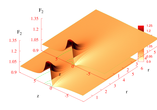
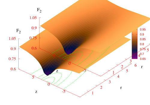
Figure 2: The profiles of the metric functions $F_{i}$ for a typical $d=6$ solution with $a=0.5$, $b=1.7$.

The Hawking temperature can be computed from the surface gravity or by requiring regularity on the Euclidean section

$$T=\frac{1}{4\pi a}\sqrt{\frac{a+b}{2}}\sqrt{\frac{F_{0}}{F_{1}}}~{},$$ (3.8)

where the constraint equation $G_{r}^{z}=0$ guarantees that the ratio $F_{0}/F_{1}$ is constant on the event horizon. At infinity, the Minkowski background is approached, with $\Delta\psi=2\pi$ there. The mass $M$ of the solutions can be read from the asymptotic expression for $f_{0}$

$$f_{0}\sim 1-\frac{16\pi GM}{(d-2)V_{d-2}(r^{2}+z^{2})^{(d-3)/4}}+\dots~{}.$$ (3.9)

The solutions satisfy also the Smarr law

$$M=\frac{d-2}{4G(d-3)}TA_{H}~{}.$$ (3.10)

All solutions we have found have $F_{2}/F_{1}\neq 1+2a/(b-a)$ for the finite $\psi-$rod. Thus, for $a\leq z\leq b$, the $(z,\psi)$ part of the metric describes a surface that is topologically $S^{2}$ with a conical singularity at one of the poles. This conical singularity prevents this black object to collapse to form a spherical black hole horizon. The value of the conical excess of $\psi$ for $a<z<b$ is

$$\delta=2\pi\left(1-\sqrt{\frac{b+a}{b-a}}\sqrt{\frac{F_{2}}{F_{1}}}\right).$$ (3.11)

We have found it convenient to introduce the quantity

$$\bar{\delta}=\frac{\delta/(2\pi)}{1-\delta/(2\pi)},$$ (3.12)

which has a finite range, $-1\leq\bar{\delta}\leq 0$, and measures the ’relative angular excess’.

     

     

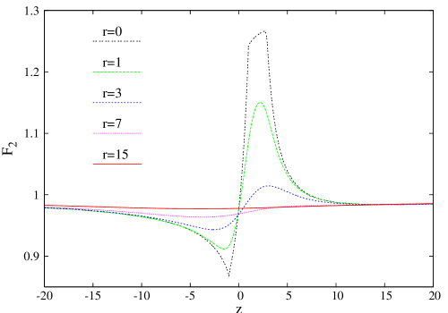
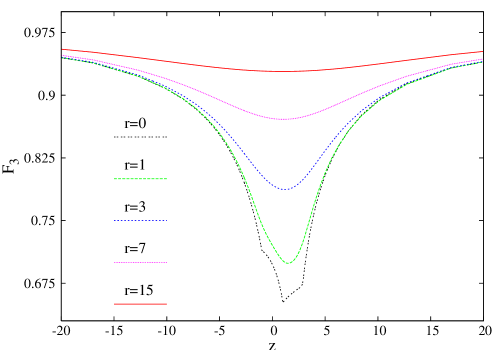
Figure 3: The metric functions $F_{i}$ are shown as a function of $z$ for several values of $r$. The relevant parameters here are $d=6$, $a=1$, $b=2.85$.

4 $d=6,7$ numerical solutions

We solve the resulting set of four coupled non-linear elliptic partial differential equations numerically, subject to the above boundary conditions. All numerical calculations are performed by using the program FIDISOL/CADSOL [21], which uses a Newton-Raphson method.

First, one introduces the new compactified coordinates $x=r/(1+r)$, $u=\arctan(z)$. The equations for $F_{i}$ are then discretized on a non-equidistant grid in $x$ and $u$. Typical grids used have sizes $80\times 160$, covering the integration region $0\leq x\leq 1$ and $-\pi/2\leq u\leq\pi/2$. (See [21] and [22] for further details and examples for the numerical procedure.) In this scheme, the input parameters are the positions of the rods fixed by $a$ and $b$ and the value $d$ of the spacetime dimension. To obtain solutions with $S^{2}\times S^{d-4}$ horizon topology, one starts with the $d=5$ solution as initial guess ($i.e.$ $F_{i}=1$) and increases the value of $d$ slowly. The iterations converge, and, in principle, repeating the procedure one obtains in this way solutions for arbitrary $d$. The physical values of $d$ are integers. We have studied solutions in $d=6,7$ dimensions in a systematic way. Solutions with $d>7$ are also likely to exist; however, their study may require a different numerical method.

     

Figure 4: (a): The scale free ratio $A_{H}/M^{(d-2)/(d-3)}$ is shown as a function of the relative angular excess $\bar{\delta}$ as defined by the relation (3.12). The value of the parameter $c_{d}$ there is $c_{d}=(d-2)/(16\pi)^{(d-2)/(d-3)}V_{d-2}^{1/(d-3)}$ and has been choosen such that the point $(1,-1)$ on the plot corresponds to the Schwarzschild-Tangerlini black hole. (b): The relative angular excess $\bar{\delta}$ is shown as a function of the ratio between the two length scales $a/b$.

The problem has two length scales $a$ and $b$, roughly corresponding to the event horizon radius and the radius of the round $\Omega$-sphere. It turns out that the above approach works well in the intermediate region of the ratio $a/b$, and fails to provide solutions with good accuracy if the two scales are widely separated or very close to each other ($i.e.$ $a/b\to 0$ or $a/b\to 1$). FIDISOL/CADSOL provides also an error estimate for each unknown function. For $d=6$, the typical numerical error for the functions is estimated to be lower than $10^{-3}$.

The Hawking temperature, event horizon area and conical excess are encoded in the values of the functions $F_{i},f_{i}^{b}$ at $r=0$. The mass parameter $M$ is computed from the asymptotic form (3.9) of the metric function $g_{tt}=-f_{0}$, the Smarr relation (3.10) being used to verify the accuracy of the solutions.

The functions $F_{i}$ change smoothly with the two parameters $a$ and $b$. Typical profiles of the solutions are presented in Figures 2, 3. One can see that the functions $F_{i}$ are smooth outside of the $z-$axis and show no sign of a singular behaviour. The crucial point here is that the divergent behaviour of $f_{i}$ was already subtracted by the background functions $f_{i}^{b}$. We have verified that the Kretschmann scalar stays finite everywhere, in particular at $r=0$.

By fixing the position of the horizon and varying the length of the finite $\psi-$rod, we have generated a branch of $d=6,7$ black objects with $S^{2}\times S^{d-4}$ horizon topology. The picture we have found is very similar to that valid for $d=5$ static black rings. First, all solutions have a conical excess $\delta$ on the finite $\psi-$rod. Moreover, on the horizon, the area of the round $S^{d-4}$-sphere is maximum for $z=-a$ and minimum at $z=a$, which shows that $\Delta\psi=2\pi$ there.

In terms of the quantity $\bar{\delta}$ as defined in (3.12), these black objects smoothly interpolate between two limits (although these regions of the parameter space are difficult to approach numerically). First, as $a/b\to 1$, one finds $\bar{\delta}\to-1$ ($i.e.$ the conical excess $\delta\to-\infty$) and the Schwarzschild-Tangherlini metric is approached (the finite $\psi-$rod vanishes). As the second $\psi-$rod extends to infinity ($a/b\to 0$), the radius on the horizon of the round $S^{d-4}$-sphere increases and asymptotically it becomes a $(d-4)$-plane, while $\bar{\delta}\to 0$. Here one expects to recover, after a suitable rescaling, the four dimensional Schwarzschild black hole uplifted to $d$ dimensions ($i.e.$ a black $(d-4)$-brane). These features are illustrated in Figure 4. For completeness, we have shown also the corresponding data for the $d=5$ static black rings.

5 Further remarks

In the absence of analytical methods to construct $d>5$ black hole solutions with nonspherical horizon topology, a numerical approach of this problem seems to be a reasonable task. In this work we have presented such a construction for $d=6,7$ static black objects with $S^{2}\times S^{d-4}$ topology of the horizon, as a first step before approaching more complex situations. The existence of the $d=6$ solution is not a surprise, since the results in [23] show that this topology is one of the few allowed for black holes in six dimensions. However, given the presence of a conical excess angle, the solutions we have found are presumably unstable and their physical relevance is obscure.

The technique proposed in this paper can easily be extended for other types of $d>5$ static black objects ($e.g.$ a superpositions of a Schwarzschild-Tangerlini black hole and a configurations with a $S^{2}\times S^{d-4}$ topology of the horizon). Also, in principle, the inclusion of rotation in this scheme is straightforward. For example, similar to the $d=5$ case, the conical singularity of the solutions with $S^{2}\times S^{d-4}$ topology of the horizon could presumably be eliminated if the $\Omega$-sphere would rotate. However, this leads to a difficult numerical problem, since the equations would depend on at least three variables. Another possible direction would be to consider more complicated versions of the static ansatz (2.1) in $d>6$ ($e.g.$ replace the angular direction $\psi$ with a sphere $S^{n}$). In the absence of rotation, one would expect such vacuum solutions to possess again some unphysical features.

Moreover, the inclusion of some matter fields is unlikely to cure the conical singularity. This is the case for the Einstein-Maxwell-dilaton generalization of the solutions here, which extremize the action

$$I=\frac{1}{16\pi G}\int d^{d}x\sqrt{-g}\left(R-\frac{1}{2}g^{\mu\nu}\partial_{\mu}\phi\partial_{\nu}\phi-\frac{1}{4}e^{-2\bar{a}\phi}F^{2}\right),$$ (5.1)

where $F=dA$. Starting with a vacuum configuration (2.1), a Harrison transformation (see $e.g.$ [24]) leads to an EMd solution with line element

$$ds^{2}~{}=-f_{0}(\cosh^{2}\beta-\sinh^{2}\beta f_{0})^{-2\alpha(d-3)}dt^{2}+(\cosh^{2}\beta-\sinh^{2}\beta f_{0})^{2\alpha}(f_{1}(dr^{2}+dz^{2})+f_{2}d\psi^{2}+f_{3}d\Omega_{d-4}^{2}),~{}{~{}}~{}$$ (5.2)

and matter fields

$$A_{\mu}=\sqrt{2(d-2)\alpha}\frac{\tanh\beta~{}e^{\bar{a}\phi_{0}}f_{0}}{\cosh^{2}\beta-\sinh^{2}\beta f_{0}}\delta_{\mu t},~{}~{}\phi=\phi_{0}-2\bar{a}(D-2)\alpha\log(\cosh^{2}\beta-\sinh^{2}\beta f_{0}),$$ (5.3)

where $\beta,~{}\phi_{0}$ are arbitrary real constants and $\alpha=(2\bar{a}^{2}(d-2)+d-3)^{-1}.$ Note that the Harrison transformation does not affect the rod structure of the metric. Thus, one finds in this way charged black objects with $S^{2}\times S^{d-4}$ topology of the horizon. For $d=5$, this is the solution presented in [8] by using a different coordinate system.

Unfortunately, one can easily see that for both $d=5$ and $d=6,7$, the line element (5.2) has the same conical singularity as the vacuum seed solution. In principle, this singularity can be removed by ”immersing” the solutions in a background gauge field, which requires to apply a second Harrison transformation (note that the resulting solutions would not be asymptotically flat; for $d=5$, such a construction has been presented in [8]). The seed solution here is (5.2), (5.3), with the electric field dualized, $\tilde{F}=e^{-2a\phi}\star F$ (with $\tilde{F}=dB$), and $\hat{\phi}=-\phi$. Then, the conical singularity vanishes for a critical value of the parameter in the second Harrison transformation. However, this last point requires knowledge of the explicit form of the magnetic potential $B$ on the $\psi$-rods, which seems not possible for the $d>5$ numerical solutions.

We close this work by remarking that, on general grounds, a numerical approach works if the length scales involved are not widely separated, which is just the opposite of the approximate construction in [16],[17]. Thus these methods are complementary. It would be interesting to construct solutions with $S^{d-3}\times S^{1}$ topology of the event horizon, which were already considered in [16]. Supposing that the static limit of these black rings can be constructed by using the ansatz (2.1), their rod structure can be read from Figure 1b by interchanging the $\psi$ and $\Omega$-rods there ($e.g.$ there is only one $\psi-$rod for $[b,\infty]$, etc.). The boundary conditions in this case are still given by (3.1)-(3.2). An unexpected feature here is that these configurations would possess no conical singularities. This difference to the static $d=5$ black rings originates in the presence of $(d-5)$ factors in the field equations (2.2)). This counter-intuitive result sheds doubt on the possibility to construct $d>5$ static black rings with a regular horizon within the ansatz (2.1) with a dependence on only two coordinates.

Acknowledgements
B.K. gratefully acknowledges support by the DFG. The work of E.R. was supported by a fellowship from the Alexander von Humboldt Foundation. E.R. would like to thank Cristian Stelea for interesting remarks on a draft of this paper.

References

- [1] R. Emparan and H. S. Reall, Phys. Rev. Lett. 88 (2002) 101101 [arXiv:hep-th/0110260].
- [2] R. Emparan and H. S. Reall, Phys. Rev. D 65 (2002) 084025 [arXiv:hep-th/0110258].
- [3] R. C. Myers and M. J. Perry, Annals Phys. 172 (1986) 304.
- [4] R. Emparan and H. S. Reall, Class. Quant. Grav. 23 (2006) R169 [arXiv:hep-th/0608012].
- [5] H. Elvang, Phys. Rev. D 68 (2003) 124016 [arXiv:hep-th/0305247].
- [6] R. Emparan, JHEP 0403 (2004) 064 [arXiv:hep-th/0402149].
- [7] H. Elvang, R. Emparan, D. Mateos and H. S. Reall, Phys. Rev. Lett. 93 (2004) 211302 [arXiv:hep-th/0407065].
-
[8]
H. K. Kunduri and J. Lucietti,
Phys. Lett. B 609 (2005) 143
[arXiv:hep-th/0412153];
S. S. Yazadjiev, arXiv:hep-th/0507097. - [9] S. S. Yazadjiev, Phys. Rev. D 73 (2006) 104007 [arXiv:hep-th/0602116].
- [10] B. Chng, R. Mann, E. Radu and C. Stelea, JHEP 0812 (2008) 009 [arXiv:0809.0154 [hep-th]].
- [11] H. Elvang and P. Figueras, JHEP 0705 (2007) 050 [arXiv:hep-th/0701035].
- [12] H. Elvang and M. J. Rodriguez, JHEP 0804 (2008) 045 [arXiv:0712.2425 [hep-th]].
- [13] H. Iguchi and T. Mishima, Phys. Rev. D 75 (2007) 064018 [arXiv:hep-th/0701043].
-
[14]
J. P. Gauntlett and J. B. Gutowski,
Phys. Rev. D 71 (2005) 025013
[arXiv:hep-th/0408010];
J. P. Gauntlett and J. B. Gutowski, Phys. Rev. D 71 (2005) 045002 [arXiv:hep-th/0408122]. -
[15]
N. A. Obers,
Lect. Notes Phys. 769 (2009) 211
[arXiv:0802.0519 [hep-th]];
R. Emparan and H. S. Reall, Living Rev. Rel. 11 (2008) 6 [arXiv:0801.3471 [hep-th]];
B. Kleihaus, J. Kunz and F. Navarro-Lerida, AIP Conf. Proc. 977 (2008) 94 [arXiv:0710.2291 [hep-th]]. - [16] R. Emparan, T. Harmark, V. Niarchos, N. A. Obers and M. J. Rodriguez, JHEP 0710 (2007) 110 [arXiv:0708.2181 [hep-th]].
- [17] R. Emparan, T. Harmark, V. Niarchos and N. A. Obers, arXiv:0902.0427 [hep-th].
- [18] T. Wiseman, Class. Quant. Grav. 20 (2003) 1137 [arXiv:hep-th/0209051].
- [19] T. Harmark, Phys. Rev. D 70 (2004) 124002 [arXiv:hep-th/0408141].
- [20] H. Kudoh, Phys. Rev. D 75 (2007) 064006 [arXiv:gr-qc/0611136].
-
[21]
W. Schönauer and R. Weiß,
J. Comput. Appl. Math. 27, 279 (1989) 279;
M. Schauder, R. Weiß and W. Schönauer, The CADSOL Program Package, Universität Karlsruhe, Interner Bericht Nr. 46/92 (1992). -
[22]
B. Kleihaus and J. Kunz,
Phys. Rev. D 57 (1998) 834
[arXiv:gr-qc/9707045];
B. Kleihaus and J. Kunz, Phys. Rev. D 57 (1998) 6138 [arXiv:gr-qc/9712086];
B. Kleihaus, J. Kunz and E. Radu, JHEP 0705 (2007) 058 [arXiv:hep-th/0702053]. - [23] C. Helfgott, Y. Oz and Y. Yanay, JHEP 0602 (2006) 025 [arXiv:hep-th/0509013].
- [24] D. V. Gal’tsov and O. A. Rytchkov, Phys. Rev. D 58 (1998) 122001 [arXiv:hep-th/9801160].