On Counteracting Byzantine Attacks
in Network Coded Peer-to-Peer Networks

Abstract

Random linear network coding can be used in peer-to-peer networks to increase the efficiency of content distribution and distributed storage. However, these systems are particularly susceptible to Byzantine attacks. We quantify the impact of Byzantine attacks on the coded system by evaluating the probability that a receiver node fails to correctly recover a file. We show that even for a small probability of attack, the system fails with overwhelming probability. We then propose a novel signature scheme that allows packet-level Byzantine detection. This scheme allows one-hop containment of the contamination, and saves bandwidth by allowing nodes to detect and drop the contaminated packets. We compare the net cost of our signature scheme with various other Byzantine schemes, and show that when the probability of Byzantine attacks is high, our scheme is the most bandwidth efficient.

I Introduction

Network coding [1], an alternative to the traditional forwarding paradigm, allows algebraic mixing of packets in a network. It maximizes throughput for multicast transmissions [2, 3, 4], as well as robustness against failures [5] and erasures [6]. Random linear network coding (RLNC), in which nodes independently take random linear combination of the packets, is sufficient for multicast networks [7], and is suitable for dynamic and unstable networks, such as peer-to-peer (P2P) networks [8, 9].

A P2P network is a cooperative network in which storage and bandwidth resources are shared in a distributed architecture. This is a cost-effective and scalable way to distribute content to a large number of receivers. One such architecture is the BitTorrent system [10], which splits large files into small blocks. After a node downloads a block, it acts as a source for that particular block. The main challenges in these systems are the scheduling and management of rare blocks.

As an alternative to current strategies for these challenges, [8, 9] propose the use of RLNC to increase the efficiency of content distribution in a P2P solution. These schemes are completely distributed and eliminate the need of a scheduler, since each node independently forwards a random linear combination. In addition, there is a high probability that each packet a node receives is linearly independent of the previous ones, and thus, the problem of redundancy caused by the flooding approaches in traditional P2P networks is reduced. RLNC based schemes significantly reduce the downloading time and improve the robustness of the system [8, 11].

Despite their desirable properties, network coded P2P systems are particularly susceptible to Byzantine attacks [12, 13, 14] – the injection of corrupted packets into the information flow. Since network coding relies on mixing of packets, a single corrupted packet may easily corrupt the entire information flow [15, 16]. Furthermore, in P2P networks, there is typically no security control over the nodes that join the network and the packets that they redistribute. The topologies of the overlay graphs that arise from traditional P2P networks are often modeled as scale-free and small-world networks [17, 18], which are prone to the dissemination of epidemics, such as worms and viruses [19, 20]. Several authors address these problems in coded P2P networks. We shall discuss these countermeasures in Section II. Most of these can be divided into two main categories: (i) end-to-end error correction and (ii) misbehavior detection.

Motivated by these observations, we address the issues of Byzantine adversaries in coded P2P networks. The main contributions of this paper are as follows:

• We propose a model for the evaluation of the impact of Byzantine attacks in coded P2P networks, and provide analytical results which show that, even for a small probability of attack, the information can become contaminated with overwhelming probability.

• We propose a new efficient, packet-based signature scheme, designed specifically for RLNC systems, to detect Byzantine attacks by checking the membership of a received packet in the valid vector space. This scheme allows an one-hop containment of the contamination.

• We analyze the overhead in terms of bandwidth associated with our signature scheme, and compare it to that of various Byzantine detection schemes. We also show that our scheme is the most bandwidth efficient if the probability of attack is high.

This paper is organized as follows. Section II gives an overview of network coding in P2P networks and existing Byzantine detection schemes. In Section III, we analyze the impact of Byzantine attacks on the system. We propose our signature scheme in Section IV, and compare its overhead with other schemes in Section V. Finally, we conclude in Section VI.

II Background

II-A Network coding in P2P networks

References [6, 7] propose a random block linear network coding system – a simple, practical capacity-achieving code, in which every node independently constructs its linear code randomly. In such a system, a source generates information in batches of $G$ packets (called a generation). The source then multicasts them to its destination nodes using RLNC, where only the packets from the same generation are mixed. Note that RLNC is a distributed protocol, which requires no state information; thus, making it suitable for dynamic and unstable networks where state information may change rapidly or may be hard to obtain.

Several authors have evaluated the performance of network coding in P2P networks. Gkantsidis et al. [9] propose a scheme for content distribution of large files in which nodes make forwarding decisions solely based on local information. This scheme improves the expected file download time and the robustness of the system. Reference [8] compares the performance of network coding with traditional coding measures in a distributed storage setting with very limited storage space with the goal of minimizing the number of storage locations a file-downloader connects to. They show that RLNC performs well without the need for a large amount of additional storage space. Dimakis et al [21] introduce a graph-theoretic framework for P2P distributed system, and show that RLNC minimizes the required bandwidth to maintain the distributed storage architectures.

II-B Byzantine detection scheme for network coded systems

II-B1 End-to-end error correction scheme

Reference [22] introduces network error correction for coded systems. They bound the maximum achievable rate in an adversarial setting, and generalize the Hamming, Gilbert-Varshamov, and Singleton bounds. Jaggi et al. [15] introduce the first distributed polynomial-time rate-optimal network codes that work in the presence of Byzantine nodes and are information-theoretically secure. The adversarial nodes are viewed as a secondary source. The source adds redundancy to help the receivers distill out the source information from the received mixtures. This work is generalized in [23, 24].

II-B2 Generation-based Byzantine detection scheme

Ho et al. [25] introduce an information-theoretic approach for detecting Byzantine adversaries, which only assumes that the adversary did not see all linear combinations received by the receivers. Their detection probability varies with the length of the hash, field size, and the amount of information unknown to the adversary. A polynomial hash is added to each packet in the generation. Once the destination node receives enough packets to decode a generation, it can probabilistically detect errors. The intuition behind this scheme is that if a packet is valid, then its data and hash are consistent with its coding vector; and a linear combination of valid packets is also valid.

II-B3 Packet-based Byzantine detection scheme

There are several signature schemes that have been presented in the literature. For instance, [8, 26, 27] use homomorphic hash functions to detect contaminated packets. Reference [16] suggests the use of a Secure Random Checksum (SRC) which requires less computation than the homomorphic hash function, but requires a secure channel to transmit the SRCs. In addition, [28] proposes a signature scheme for network coding based on Weil pairing on elliptic curves.

III Impact of Byzantine attacks on P2P networks

In this section, we first introduce our model for evaluating the probability of a distributed denial of service attack (DDoS) caused by Byzantine nodes in a P2P network. We then present results for two distinct scenarios.

III-A Model

We consider a directed graph with a set of nodes $\cal N$. A source node has a large file to be sent to receiver nodes. The file is divided into $m$ packets. To do so, the source connects to a subset of nodes, $\mathcal{N}_{s}\subseteq\cal N$, chosen uniformly at random, and sends each of them a different random linear combination of the original file packets. To ensure that enough degrees of freedom exist in the network, $|\mathcal{N}_{s}|\geq m$. We refer to the nodes in $\mathcal{N}_{s}$ as level-s nodes. A tracker node keeps track of the list of informed nodes, $N(t)$, i.e., nodes that keep an information packet.

For a receiver to retrieve the file, it connects to a subset of nodes $\mathcal{N}_{r}\subseteq\cal N$, chosen uniformly at random, with $|\mathcal{N}_{r}|\geq|\mathcal{N}_{s}|$. We refer to the nodes in $\mathcal{N}_{r}$ as level-r nodes. Note that there may be an overlap between level-s and level-r. In each time slot, one of the uninformed level-r nodes, $n\in\mathcal{N}_{r}\setminus\mathcal{N}_{s}$, contacts the tracker to retrieve a random list of $d$ informed nodes, where $d<|\mathcal{N}_{s}|$. The node $n$ then connects to these informed nodes through a secure overlay connection, retrieves their packets, and stores a single random linear combination of these packets. During the same time slot, the tracker updates its list of informed nodes to $N(t)\cup\{n\}$. This process is repeated for all nodes in $\mathcal{N}_{r}\setminus\mathcal{N}_{s}$, and then all level-r nodes forward their stored packets to the receiver. In order to maximize the probability of storing linearly independent combinations in level-r nodes and ensure decodability at the receiver, we set $d\geq 2$. Although we assume that each node in level-s and level-r stores only one packet, the model can be easily generalized to account for higher numbers. An example of this network model is shown in Figure 1. Note that the tracker is considered to be a trusted party in our model – in fact, as in the case of most P2P protocols, a dishonest tracker would yield a protocol failure with overwhelming probability.

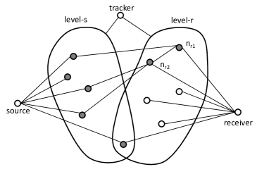
Figure 1: Network model. The source is connected to the level-s nodes, and the receiver is connected to the level-r nodes. The dark nodes are the informed nodes. The level-r nodes take turns to contact the tracker, and connects to $|D|=2$ level-s nodes based on the list returned by the tracker. Here, nodes $n_{r1}$ and $n_{r2}$ has completed this process, and the other level-r nodes have not.

We define an Information Contact Graph $G(t)=\{N(t),A(t)\}$ to denote the evolving graph formed in the above process, where $N(t)$ is the list of informed nodes and $A(t)$ is the set of overlay links that connect the level-s and level-r nodes. The probability that a node becomes a Byzantine attacker is $p_{b}$. An attacker corrupts the packet it stores by generating arbitrary content while complying to the standard packet format. A node independently decides whether it becomes Byzantine at the start of the file dissemination process according to $p_{b}$ and stays that way throughout the process. We define an indicator variable $I_{b}(n)$ which is 1 if node $n$ is Byzantine and 0 otherwise. The tracker has no information about which nodes are Byzantine. A contaminated packet is a packet that is either directly corrupted by an attacker, or is a linear combination that involves at least one contaminated packet. A contaminated node is a node that stores a contaminated packet. The blocking probability $\Psi$ is the probability that the receiver collects at least one contaminated packet, and thus, is unable to decode the file. This is equivalent to the probability that the attacker successfully carries out a DDoS attack.

III-B Analysis of Impact of Byzantine Attacks

We now evaluate the blocking probability at the receiver. We then consider the expected number of contaminated nodes at any given time. First, we introduce necessary definitions, as follows. We define an indicator variable $I_{c}(t,n)$ which is equal to $1$ if node $n$ is contaminated at time $t$ and $0$ otherwise. $C({t})$ is a random variable for the number of contaminated nodes in $N({t})$, and $\overline{C}({t})=|N({t})|-C({t})$ is the number of uncontaminated nodes. The function $h(k;N,m,n)$ denotes the hypergeometric distribution, in which

$$h(k;N,m,n)=\dbinom{m}{k}\dbinom{N-m}{n-k}/\dbinom{N}{m}.$$

Let $N_{b}$ denote the number of informed Byzantine nodes at time $t=0$, that is, the number of Byzantine nodes in $\mathcal{N}_{s}$. $N_{b}$ has a binomial distribution with parameters $(|\mathcal{N}_{s}|,p_{b})$.

We consider two scenarios. In Theorem 1, for simplicity, we consider a static informed nodes list, in which the list kept by the tracker is fixed to $\mathcal{N}_{s}$. In this case, level-r nodes only connect to level-s nodes. Second, in Theorem 2, we generalize to the case in which the tracker updates its list of informed nodes to $N({t})$, as stated in Section III-A.

Theorem 1 (Static Informed Nodes List)

Let $G(t)$ be an information contact graph in which nodes in $\mathcal{N}_{r}$ only connect to nodes in $\mathcal{N}_{s}$. Then its blocking probability $\Psi$ is given by:

$$\Psi=1-\sum_{y=0}^{|\mathcal{N}_{s}|}h(y;|\mathcal{N}|,|\mathcal{N}_{s}|,|\mathcal{N}_{r}|)\left(\sum_{i=0}^{|\mathcal{N}_{s}|}\dbinom{|\mathcal{N}_{s}|}{i}p_{b}^{i}(1-p_{b})^{|\mathcal{N}_{s}|-i}f(i,y)\right),$$

where

$$f(i,y)=\left(1-\frac{i}{|\mathcal{N}_{s}|}\right)^{y}\bigg{[}(1-p_{b})h(0,|\mathcal{N}_{s}|,i,d)\bigg{]}^{|\mathcal{N}_{r}|-y}.$$

Proof:

We consider two disjoint subsets of $\mathcal{N}_{r}$: the set of informed nodes at $t=0$, that is, $\mathcal{N}_{r}\cap\mathcal{N}_{s}$, and the uninformed nodes, that is, $\mathcal{N}_{r}\backslash\mathcal{N}_{s}$. Let $Y$ be a random variable for the number of nodes in $\mathcal{N}_{r}\cap\mathcal{N}_{s}$. $Y$ has a hypergeometric distribution, $P(Y=y)=h(y;|\mathcal{N}|,|\mathcal{N}_{s}|,|\mathcal{N}_{r}|)$.

We first consider $n\in\mathcal{N}_{r}\cap\mathcal{N}_{s}$. Given $N_{b}=i$ and $Y=y$, the probability that $n$ is uncontaminated is equal to the probability that it is not initially Byzantine, which is equal to $1-i/|\mathcal{N}_{s}|$. Then, the probability that all nodes in $\mathcal{N}_{r}\cap\mathcal{N}_{s}$ are uncontaminated is:

$$P({I_{c}({n,0})=0},\forall n\in\mathcal{N}_{r}\cap\mathcal{N}_{s}|N_{b}=1,Y=y)=\left(1-\frac{i}{|\mathcal{N}_{s}|}\right)^{y}.$$

Now, at each timeslot $t>0$, a node $n\in\mathcal{N}_{r}\backslash\mathcal{N}_{s}$ becomes informed. For $n$ to be uncontaminated, it must not be Byzantine and it must connect to $d$ uncontaminated nodes. Then,

$$P({I_{c}({n,t})=0}|N_{b}=i,Y=y)=(1-p_{b})h(0,|\mathcal{N}_{s}|,i,d).$$

It follows that the probability that all nodes in $\mathcal{N}_{r}\backslash\mathcal{N}_{s}$ are uncontaminated at time $t$ is:

$$P({I_{c}({n,t})=0},\forall n\in\mathcal{N}_{r}\backslash\mathcal{N}_{s}|N_{b}=i,Y=y)=\bigg{(}(1-p_{b})h(0,|\mathcal{N}_{s}|,i,d)\bigg{)}^{t},\text{ for }0\leq t\leq|\mathcal{N}_{r}|-y.$$

Note that since $|\mathcal{N}_{r}\backslash\mathcal{N}_{s}|$ nodes are added, the information dissemination process ends at $t=|\mathcal{N}_{r}|-y$. Now, the probability that only uncontaminated nodes exist in $\mathcal{N}_{r}$ at time $t=|\mathcal{N}_{r}|-y$, conditioned on $Y=y$ and $N_{b}=i$, is:

$$f(i,y)=\left(1-\frac{i}{|\mathcal{N}_{s}|}\right)^{y}\bigg{[}(1-p_{b})h(0,|\mathcal{N}_{s}|,i,d)\bigg{]}^{|\mathcal{N}_{r}|-y}.$$

$N_{b}$ has a binomial distribution, $Y$ has a hypergeometric distribution and they are independent of each other. Taking out these two conditions, the probability that all nodes in $\mathcal{N}_{r}$ are uncontaminated is:

$$\gamma=\sum_{y=0}^{|\mathcal{N}_{s}|}h(y;|\mathcal{N}|,|\mathcal{N}_{s}|,|\mathcal{N}_{r}|)\left(\sum_{i=0}^{|\mathcal{N}_{s}|}\dbinom{|\mathcal{N}_{s}|}{i}p_{b}^{i}(1-p_{b})^{|\mathcal{N}_{s}|-i}f(i,y)\right).$$

It follows that the blocking probability is $\Psi=1-\gamma$. ∎

We now consider that the list of informed nodes at the tracker is $N({t})$, that is, it is updated with each new informed level-r node.

Theorem 2 (Evolving informed nodes list)

Let $G(t)$ be an information contact graph in which $|\mathcal{N}_{r}\backslash\mathcal{N}_{s}|$ are to be added to the graph by connecting to nodes in $N({t})$. Then its blocking probability $\Psi$ is:

$$\Psi=1-\sum_{y=0}^{|\mathcal{N}_{s}|}h(y;|\mathcal{N}|,|\mathcal{N}_{s}|,|\mathcal{N}_{r}|)\left(\sum_{i=0}^{|\mathcal{N}_{s}|}\dbinom{|\mathcal{N}_{s}|}{i}p_{b}^{i}(1-p_{b})^{|\mathcal{N}_{s}|-i}f(i,y)\right),$$

where

$$f(i,y)=\left(1-\frac{i}{|\mathcal{N}_{s}|}\right)^{y}\Bigg{[}\prod_{t=1}^{|\mathcal{N}_{r}|-y}(1-p_{b})h(0;|\mathcal{N}_{s}|+t-1,i,d)\Bigg{]}.$$

Proof:

Recall from Theorem 1 that we consider two disjoint subsets of $\mathcal{N}_{r}$, that is, $\mathcal{N}_{r}\cap\mathcal{N}_{s}$ and $\mathcal{N}_{r}\backslash\mathcal{N}_{s}$. As before, $Y$ is the number of nodes in $\mathcal{N}_{r}\cap\mathcal{N}_{s}$. Again, at time $t=0$, the probability that all nodes in $\mathcal{N}_{r}\cap\mathcal{N}_{s}$ are uncontaminated given $N_{b}=i$ and $Y=y$ is $(1-i/|\mathcal{N}_{s}|)^{y}$.

We now consider the nodes in $\mathcal{N}_{r}\backslash\mathcal{N}_{s}$ and assume $N_{b}=i,Y=y$. At each time step, there are $C({t})$ contaminated nodes and $\overline{C}({t})=|\mathcal{N}_{s}|+t-C({t})$ uncontaminated nodes in $N({t})$. The probability of obtaining a contaminated node at time $t+1$ is only dependent on $C({t})$ and $\overline{C}({t})$, and thus, we can model these probabilities by Markov chains $\Xi|{N_{b},Y}=\{S,\mathbf{P}\}$, in which $S$ represents the set of states and $\mathbf{P}$ represents the matrix of transition probabilities. A state in $S$ is represented by $s=(C({t}),\overline{C}({t}))$. Transitions from $s$ are only possible to $s^{\prime}=(C({t})+1,\overline{C}({t}))$ and to $s^{\prime\prime}=(C({t}),\overline{C}({t})+1)$. It is also important to note that the depth of the Markov chain is equal to $|\mathcal{N}_{r}\backslash\mathcal{N}_{s}|=|\mathcal{N}_{r}|-y$. The transition probabilities from $s$ when adding a node $n$ are $P(s\rightarrow s^{\prime})=P({I_{c}({t+1,n})=1}|C({t}),\overline{C}({t}),N_{b},Y)$ and $P(s\rightarrow s^{\prime\prime})=P({I_{c}({t+1,n})=0}|C({t}),\overline{C}({t}),N_{b},Y)$. $\Xi|N_{b},Y$ is illustrated in  Figure 2 for $|\mathcal{N}_{r}\backslash\mathcal{N}_{s}|=2$.

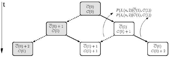
Figure 2: Markov diagram for the dissemination process, $|\mathcal{N}_{r}|-Y=2$. The transitions to the left (dotted arrows) represent the addition of an uncontaminated node, and the transitions to the right (filled arrows) represent the addition of a contaminated node. The grey states are considered in computing $\Psi$, that is, the states in which no contaminated nodes are added.

Let us denote $C({t})$ as $x$ and $t^{\prime}=|\mathcal{N}_{s}|+t$, it follows that $\overline{C}({t})=t^{\prime}-x$. Now let $p_{\{s\}}^{t}$ denote the probability of being in state $s$ at time $t$. $p_{\{s\}}^{t}=p_{\{x,t-x\}}^{t}$ can be defined recursively as:

$$\begin{cases}p_{\{x,t^{\prime}-x\}}^{t}=p_{\{x-1,t^{\prime}-x\}}^{t-1}p_{(\{x-1,t^{\prime}-x\}\rightarrow\{x,t^{\prime}-x\})}+p_{\{x,t^{\prime}-x-1\}}^{t-1}p_{(\{x,t^{\prime}-x-1\}\rightarrow\{x,t^{\prime}-x\})},\\ p_{(\{x,t^{\prime}-x\}\rightarrow\{x+1,t^{\prime}-x\})}=1-P({I_{c}({t,n})=0}|x,t^{\prime}-x,N_{b}=i,Y=y),\\ p_{(\{x,t^{\prime}-x\}\rightarrow\{x,t^{\prime}-x+1\})}=P({I_{c}({t,n})=0}|x,t^{\prime}-x,N_{b}=i,Y=y),\\ p_{\{i,|\mathcal{N}_{s}|-i\}}^{0}=1.\end{cases}$$

Now, consider that node $n$ is active at time $t$. The probability of $n$ being uncontaminated is the probability that it is not Byzantine and does not connect to contaminated nodes. Thus,

$$P({I_{c}({t,n})=0}|\overline{C}({t-1}),C({t-1}),N_{b}=i,Y=y) = (1-p_{b})h(0;|\mathcal{N}_{s}|+t-1,C({t-1}),d).$$

Now, notice that the probability of only having uncontaminated nodes at time $t=|\mathcal{N}_{r}|-y$ is the probability of, starting in state $(C({0}),\overline{C}({0}))=(i,|\mathcal{N}_{s}|-i)$, ending in state $(i,|\mathcal{N}_{s}|-i+|\mathcal{N}_{r}|-y)$ after $|\mathcal{N}_{r}|-y$ steps: in that case, no contaminated node is added to the network. The probability of this event, conditioned on $N_{b}=i$ and $Y=y$, is

$$\prod_{t=1}^{|\mathcal{N}_{r}|-y}P({I_{c}({t,n})=0}|\overline{C}({t-1}),C({t-1}),N_{b}=i,Y=y)=\prod_{t=1}^{|\mathcal{N}_{r}|-y}(1-p_{b})h(0;|\mathcal{N}_{s}|+t-1,i,d).$$

Combining the results for sets $\mathcal{N}_{r}\cap\mathcal{N}_{s}$ and $\mathcal{N}_{r}\backslash\mathcal{N}_{s}$, we have that the probability that no contaminated nodes exist in $\mathcal{N}_{r}$ given that $N_{b}=i$ and $Y=y$ is given by

$$f(i,y)=\left(1-\frac{i}{|\mathcal{N}_{s}|}\right)^{y}\Bigg{[}\prod_{t=1}^{|\mathcal{N}_{r}|-y}(1-p_{b})h(0;|\mathcal{N}_{s}|+t-1,i,d)\Bigg{]}.$$

Finally, it follows that the blocking probability at time $|\mathcal{N}_{r}\backslash\mathcal{N}_{s}|$ is

$$\Psi=1-\sum_{y=0}^{|\mathcal{N}_{s}|}h(y;|\mathcal{N}|,|\mathcal{N}_{s}|,|\mathcal{N}_{r}|)\left(\sum_{i=0}^{|\mathcal{N}_{s}|}\dbinom{|\mathcal{N}_{s}|}{i}p_{b}^{i}(1-p_{b})^{|\mathcal{N}_{s}|-i}f(i,y)\right).$$

∎

The results from Theorems 1 and 2 are illustrated in Figure 3. Note that even for a small $p_{b}$, the blocking probability $\Psi$ is very high. Even for the case in Theorem 1, $\Psi$ grows exponentially. This is because it is sufficient for a single level-r node to connect to a Byzantine node in level-s to contaminate the receiver. Figure 3 indicates that $\Psi$ grows faster for the evolving informed node list than for the static informed node list). This is due to the fact that as more nodes are added to the network, the presence of contaminated nodes becomes more likely, and thus, the probability that a level-r node connects to at least one contaminated node increases. The probability $\Psi$ also increases with other parameters such as $d$, $|\mathcal{N}_{s}|$, and $|\mathcal{N}_{r}|$ since they increase the probability of level-r nodes connecting to contaminated nodes.

From the above proofs, it follows that the number of contaminated nodes in $N({t}),t>0$, is dependent on the random variable $Y=|\mathcal{N}_{r}\cap\mathcal{N}_{s}|$. We now perform an analysis of the expected number of contaminated nodes in the network $E[C({t})]$ conditioned on $Y=y$.

First, we consider the case of the static informed nodes list, conditioned on $N_{b}=i,Y=y$. It is clear that $E[C({0})|N_{b}=i]=i$. Now, at each time step $t$, one contaminated node is added to $N({t})$ with probability $1-P({I_{c}({n,t})=0}|N_{b}=i,Y=y)$ and thus $E[C({t})|N_{b}=i,Y=y]=i+t(1-(1-p_{b})h(0;|\mathcal{N}_{s}|,i,d))$. It follows that

$$E[C({t})|Y=y]=\sum_{i=0}^{|\mathcal{N}_{s}|}\dbinom{|\mathcal{N}_{s}|}{i}p_{b}^{i}(1-p_{b})^{|\mathcal{N}_{s}|-i}\bigg{(}i+t(1-(1-p_{b})h(0;|\mathcal{N}_{s}|,i,d))\bigg{)}.$$

In the case of the evolving informed nodes list, since the states of $\Xi|N_{b},Y$ are representative of the number of contaminated nodes in the network, $E[C({t})|N_{b},Y]$ has a direct correspondence to the expected state the Markov Chain is in after $t$ time steps; therefore:

$$E[C({t})|Y=y]=\sum_{i=0}^{|\mathcal{N}_{s}|}\dbinom{|\mathcal{N}_{s}|}{i}p_{b}^{i}(1-p_{b})^{|\mathcal{N}_{s}|-i}\bigg{(}\sum_{x=i}^{i+t}xp^{t}_{\{x,t^{\prime}-x\}}\bigg{)}.$$

In order to visualize these results, we take the expected value of $Y$ for the set of parameters chosen in Figure 3, which is equal to 1. Then, we plot $E[C({t})|Y=1]$ for the static and evolving informed node lists. It is shown in Figure 4 that the expected number of contaminated nodes in the static case is linear with time. For small probabilities $p_{b}$, the $E[C({t})|Y=1]$ is higher for the evolving case; as $p_{b}$ increases, the values for both cases become similar.

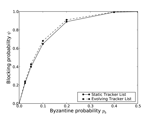
Figure 3: Blocking probability in function of $p_{b}$ for $|\mathcal{N}|=30$, $|\mathcal{N}_{s}|=5$, $|\mathcal{N}_{r}|=6$ and $d=3$. The results for the static and evolving informed nodes list are shown in full and dashed, respectively.

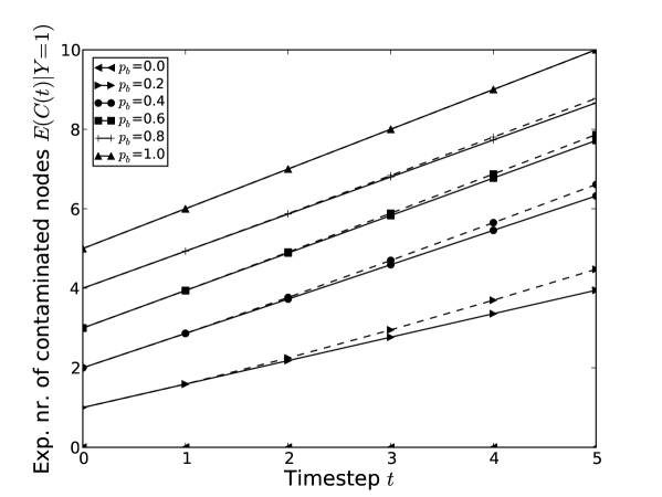
Figure 4: Expected number of contaminated nodes in function of time, for $|\mathcal{N}|=30$, $|\mathcal{N}_{s}|=5$, $|\mathcal{N}_{r}|=6$, $d=3$ and $Y=1$. The results for the static and evolving informed nodes list are shown in full and dashed, respectively.

IV Signature scheme for Byzantine detection

From the previous Section, we can see that coded P2P networks are highly vulnerable to Byzantine attacks, and the contamination can quickly spread throughout the network. Although we only consider a particular network model in Section III for the purpose of analysis, such problems exist in all network coded systems. Therefore, it is desirable to have a signature scheme that checks the validity of each received packet without decoding the whole file. Then the contamination can be contained in one-hop, and we can avoid the decoding delay. In uncoded systems, the source knows all the packets being transmitted in the network, and therefore, can sign each one of them. However, in a coded system, each node produces “new” packets, and standard digital signature schemes do not apply. Previous work that attempts to solve this problem is based on homomorphic hash functions [8, 26, 27], Secure Random Checkup [16], or Weil pairing on elliptic curves [28]. In this section, we introduce a novel signature scheme for the coded system based on the Discrete Logarithm problem.

We consider a directed graph with a set of nodes $\cal N$. A source node has a large file to be sent to receiver nodes. The file is divided into $m$ packets. A node in the network receives linear combinations of the packets from the source or from other nodes. In this framework, a node is also a server to packets it has downloaded, and always sends out random linear combinations of all the packets it has obtained so far to other nodes. When a receiver has received $m$ linearly independent packets, it can re-construct the whole file. We denote the $m$ original packets as $\mathbf{\bar{v}}_{1},...,\mathbf{\bar{v}}_{m}$, and view them as elements in $l$-dimensional vector space $\mathbb{F}_{p}^{l}$, where $p$ is a prime. The source node adds coding vectors to create ${\mathbf{v}}_{1},...,{\mathbf{v}}_{m}$, ${\mathbf{v}}_{i}=(0,...,1,...,0,{\bar{v}}_{i1},...,{\bar{v}}_{il})$, where the first $m$ elements are zero except the $i$th element which is 1, and $\bar{v}_{ij}\in\mathbb{F}_{p}$ is the $j$th element in $\mathbf{\bar{v}}_{i}$. A packet ${\mathbf{w}}$ received by a node is a linear combination of these vectors,

$${\mathbf{w}}=\sum_{i=1}^{m}\beta_{i}{\mathbf{v}}_{i},$$

where $(\beta_{1},...,\beta_{m})$ is the global coding vector.

The key observation for our signature scheme is that the vectors ${\mathbf{v}}_{1},...,{\mathbf{v}}_{m}$ span a subspace $V$ of ${\mathbb{F}}_{p}^{m+l}$, and a received vector ${\mathbf{w}}$ is a valid linear combination of vectors ${\mathbf{v}}_{1},...,{\mathbf{v}}_{m}$ if and only if it belongs to $V$. Our scheme is based on standard modulo arithmetic (in particular the hardness of the Discrete Logarithm problem) and on an invariant signature for the linear span $V$. Each node verifies the integrity of a received vector ${\mathbf{w}}$ by checking the membership of ${\mathbf{w}}$ in $V$ based on the signature.

Our signature scheme is defined by the following ingredients:

• $q$: a large prime number such that $p$ is a divisor of $q-1$. Note that standard techniques, such as that used in Digital Signature Algorithm (DSA) [29], apply to find such $q$.

• $g$: a generator of the group $G$ of order $p$ in ${\mathbb{F}}_{q}$. Since the order of the multiplicative group ${\mathbb{F}}_{q}^{*}$ is $q-1$ (a multiple of $p$), we can always find a subgroup, $G$, with order $p$ in ${\mathbb{F}}_{q}^{*}$.

• Private key: ${\mathbf{K}}_{s}=\{\alpha_{i}\}_{i=1,...,m+l}$, a random set of elements in ${\mathbb{F}}^{*}_{p}$, only known to the source.

• Public key: ${\mathbf{K}}_{p}=\{h_{i}=g^{\alpha_{i}}\}_{i=1,...,m+l}$, signed by some standard signature scheme, e.g., DSA, and published by the source.

To distribute a file in a secure manner, the signature scheme works as follows.

1. Using the vectors ${\bf v}_{1},...,{\bf v}_{m}$ from the file, the source finds a vector ${\mathbf{u}}=(u_{1},...,u_{m+l})\in{\mathbb{F}}_{p}^{m+l}$ orthogonal to all vectors in $V$. Specifically, the source finds a non-zero solution, ${\bf u}$, to the set of equations ${\bf v}_{i}\cdot{\bf u}=0$ for $i=1,...,m$.

2. The source computes the vector ${\mathbf{x}}=(u_{1}/\alpha_{1},u_{2}/\alpha_{2},...,u_{m+l}/\alpha_{m+l})$.

3. The source signs ${\mathbf{x}}$ with some standard signature scheme and publishes ${\bf x}$. We refer to the vector ${\bf x}$ as the signature of the file being distributed.

4. The client node verifies that ${\bf x}$ is signed by the source.

5. When a node receives a vector ${\mathbf{w}}$ and wants to verify that ${\mathbf{w}}$ is in $V$, it computes

   $$d=\prod_{i=1}^{m+l}h_{i}^{x_{i}w_{i}},$$

   and verifies that $d=1$.

To see that $d$ is equal to 1 for any valid ${\mathbf{w}}$, we have

$$d=\prod_{i=1}^{m+l}h_{i}^{x_{i}w_{i}}=\prod_{i=1}^{m+l}(g^{\alpha_{i}})^{u_{i}w_{i}/\alpha_{i}}=\prod_{i=1}^{m+l}g^{u_{i}w_{i}}=g^{\sum_{i=1}^{m+l}(u_{i}w_{i})}=1,$$

where the last equality comes from the fact that ${\mathbf{u}}$ is orthogonal to all vectors in $V$.

Next, we show that the system described above is secure. In essence, the theorem below shows that given a set of vectors that satisfy the signature verification criterion, it is provably as hard as the Discrete Logarithm problem to find new vectors that also satisfy the verification criterion other than those that are in the linear span of the vectors already known.

Definition 1

Let $p$ be a prime number and $G$ be a multiplicative cyclic group of order $p$. Let $k$ and $n$ be two integers such that $k<n$, and ${\bf\Gamma}=\{h_{1},...,h_{n}\}$ be a set of generators of $G$. Given a linear subspace, $V$, of rank $k$ in ${\mathbb{F}}_{p}^{n}$ such that for every ${\mathbf{v}}\in V$, the equality ${\bf\Gamma}^{\mathbf{v}}\triangleq\prod_{i=1}^{n}h_{i}^{v_{i}}=1$ holds, we define the $(p,k,n)$-Diffie-Hellman problem as the problem of finding a vector ${\mathbf{w}}\in{\mathbb{F}}_{p}^{n}$ with ${\bf\Gamma}^{\mathbf{w}}=1$ but ${\mathbf{w}}\notin V$.

By this definition, the problem of finding an invalid vector that satisfies our signature verification criterion is a $(p,m,m+l)$-Diffie-Hellman problem. Note that in general, the $(p,n-1,n)$-Diffie-Hellman problem has no solution. This is because if $V$ has rank $n-1$ and a ${\bf w^{\prime}}$ exists such that ${\bf\Gamma}^{\mathbf{w}^{\prime}}=1$ and ${\mathbf{w}^{\prime}}\notin V$, then $w^{\prime}+V$ spans the whole space, and any vector ${\bf w}\in{\mathbb{F}}_{p}^{n}$ would satisfy ${\bf\Gamma}^{\mathbf{w}}=1$. This is clearly not true, therefore, no such ${\bf w^{\prime}}$ exists.

Theorem 3

For any $k<n-1$, the $(p,k,n)$-Diffie-Hellman problem is as hard as the Discrete Logarithm problem.

Proof:

Assume there exists an efficient algorithm to solve the $(p,k,n)$-Diffie-Hellman problem, and we wish to compute the discrete logarithm $\log_{g}(z)$ for some $z=g^{x}$, where $g$ is a generator of a cyclic group $G$ with order $p$. We can choose two random vectors ${\mathbf{r}}=(r_{1},...,r_{n})$ and ${\mathbf{s}}=(s_{1},...,s_{n})$ in ${\mathbb{F}}_{p}^{n}$, and construct ${\bf\Gamma}=\{h_{1},...,h_{n}\}$, where $h_{i}=z^{r_{i}}g^{s_{i}}$ for $i=1,...,n$. We then find $k$ linearly independent (and otherwise random) solutions ${\mathbf{v}}_{1},...,{\mathbf{v}}_{k}$ to the equations

$${\mathbf{v}}\cdot{\mathbf{r}}=0\;\;\mbox{and}\;\;{\mathbf{v}}\cdot{\mathbf{s}}=0.$$

Note that there exist $n-2$ linearly independent vector solutions to the above equations. Let $V$ be the linear span of $\{{\mathbf{v}}_{1},...,{\mathbf{v}}_{k}\}$, then any vector ${\mathbf{v}}\in V$ satisfies ${\bf\Gamma}^{\mathbf{v}}=1$. Now, if we have an algorithm for the $(p,k,n)$-Diffie-Hellman problem, we can find a vector ${\mathbf{w}}\notin V$ such that ${\bf\Gamma}^{\mathbf{w}}=1$. This vector would satisfy ${\mathbf{w}}\cdot(x{\mathbf{r}}+{\mathbf{s}})=0$. Since ${\mathbf{r}}$ is statistically independent from $(x{\mathbf{r}}+{\mathbf{s}})$, with probability greater than $1-1/p$, we have ${\mathbf{w}}\cdot{\mathbf{r}}\neq 0$. In this case, we can compute

$$\log_{g}(z)=x=\frac{{\mathbf{w}}\cdot{\mathbf{s}}}{{\mathbf{w}}\cdot{\mathbf{r}}}.$$

This means the ability to solve the $(p,k,n)$-Diffie-Hellman problem implies the ability to solve the Discrete Logarithm problem. ∎

This proof is an adaptation of a proof in an earlier publication by Boneh et. al [30].

Our signature scheme makes use of the linearity property of RLNC, and enables the nodes to check the integrity of packets without a secure channel, unlike the homomorphic hash function or SRC schemes [16, 26]. In addition, our scheme does not require the nodes to decode coded packets to check their validity – thus, is efficient in terms of delay. The computation involved in the signature generation and verification processes is very simple. Furthermore, our scheme uses the Discrete Logarithm problem, which is more standardized and widely used, compared to the recently developed Weil pairing problem used in [28]. Lastly, we note that our signature scheme is rateless, which is not the case in end-to-end or generation based detection schemes.

V Overhead analysis

In the previous Sections, we showed that our signature scheme is beneficial, as even a small amount of attack can have a devastating effect in coded networks. However, we have not shown that this scheme is efficient in terms of bandwidth (i.e. overhead of augmenting the signature scheme), and indeed, it is not always the case that our signature scheme is desirable. We now study the cost and benefit of the following three Byzantine schemes: 1) our signature scheme proposed in Section IV, 2) end-to-end error correction scheme [15], and 3) generation-based Byzantine detection scheme [6]. If we implement Byzantine detection schemes, we can detect contaminated data, drop them, and therefore, only transmit valid data; however, this benefit comes with the overhead of the schemes in the forms of hashes and signatures. It is important to note that, for the dropped data, the receivers perform erasure correction, which is computationally lighter than error correction; thus, there is no need of retransmissions.

We consider a node $n\in\mathcal{N}$ in the network as in Section IV. Node $n$ wishes to check the validity of the data it forwards. Assume that node $n$ receives $M$ packets per time slot. Recall that $m$ is the number of packets in a file and $l$ is the length of each packet, therefore, each packet consists of $(m+l)$ symbols. If $n$ detects an error, then it discards that data; otherwise, it forwards the data. The probability that $n$ receives a contaminated packet is $p_{n}$ as shown in Figure 5. Note that the probability $p_{n}$ of an attack is topology dependent. However, in order to compare the performance of various schemes, we use a generic per node model to examine the overhead incurred at a node. We assume that there is an external model of vulnerability which gives an estimate of $p_{n}$. Note that the blocking probability $\Psi$ analyzed in Section III provides such an estimate.

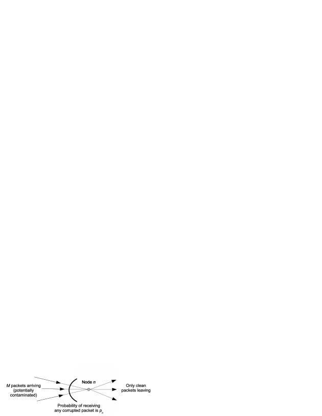
Figure 5: Diagram of a node $n$ in a network

V-A Overhead analysis of our packet-based signature scheme

We examine the overhead incurred by our signature scheme. Recall from Section IV, the file size is $ml\log{p}$ bits. The file is divided into $m$ packets, each of which is a vector in $\mathbb{F}_{p}^{l}$. Thus, the overhead of the RLNC scheme is $m/l$ times the file size, and in practical networks $m\ll l$.

The initial setup of our signature scheme involves the publishing of the public key, ${\bf K}_{p}$, which is $(m+l)\log(q)$ bits. In typical cryptographic applications, the sizes of $p$ and $q$ are 20 bytes (160 bits) and 128 bytes (1024 bits), respectively; thus, the size of ${\bf K}_{p}$ is approximately $6(m+l)/ml$ times the file size. This overhead is negligible as long as $6\ll m\ll n$. For example, if we have a file of size 10MB, divided into $m=100$ packets, then the overhead is approximately 6%. We note that the public key ${\bf K}_{p}$ cannot be fully reused for multiple files, as it is possible for a malicious node to generate a vector which is not a valid linear combination of the original vectors yet satisfies the check $d=1$ using information obtained from previously downloaded files. We do not provide the details of this for want of space.

To prevent this from happening, we can redistribute keys for each additional file in one of the two methods below. The first method consists of publishing a new public key ${\bf K}_{p}$ for each file, which would incur an overhead of $6(m+l)/ml$ times the file size. Note that if we republish ${\bf K}_{p}$ for every file, we can reuse the signature ${\bf x}$. The second method is to update ${\bf K}_{p}$ partially and generate a new ${\bf x}$ for each file. This incurs less overhead than the previous method, however, requires a high variability in ${\bf w}$ for it to be secure. This update incurs negligible amount of overhead as well. For example, for a 10MB file, the overhead is less than 0.1%.

The initial ${\bf K}_{p}$ distribution costs approximately 6% of our file size, and the incremental update of ${\bf K}_{p}$ and ${\bf x}$ is much less than 6% if we use the second method. Therefore, we shall denote the overhead associated with our signature by $o_{p}\triangleq\frac{6}{100}(m+l)$ symbols per packet, i.e. 6% overhead.

If $n$ detects an error in a packet, then it discards it – by doing so, $n$ can filter out all the contaminated packets and use its bandwidth to transmit only valid packets. Therefore, $n$ only forwards on average $1-\frac{o_{p}}{m+l}$ fraction of the data received.

Our signature scheme costs $o_{p}M$ symbols per time slot. However, by discarding the contaminated packets, node $n$ can on average save its bandwidth by $M(m+l)p_{n}$ symbols per time slot. Therefore, the net cost of the signature scheme as a fraction of the total data received is:

$$\frac{\max\{0,Mo_{p}-M(m+l)p_{n})\}}{M(m+l)}=\frac{\max\{0,o_{p}-(m+l)p_{n}\}}{m+l}.$$ (1)

When $p_{n}$ is high, then checking each packet for error saves on bandwidth – i.e. $(o_{p}-(m+l)p_{n})<0$, which shows that the cost of the signature scheme is canceled by the bandwidth gained from dropping the corrupted packets. Therefore, this approach is the most sensible when the network is unreliable or under heavy attack.

V-B Overhead analysis of end-to-end error correction

In this subsection, we shall use the rate-optimal error correction codes from Jaggi et al. [15]. As long as the attack is within the network capacity, this scheme allows the intermediate nodes to transmit at the remaining network capacity, i.e. the end-to-end network capacity minus the capacity the adversary can contaminate. In this scenario, node $n$ just naively performs RLNC and forwards the data it has received. Therefore, node $n$ transmits on average $M(m+l)p_{n}$ contaminated symbols. Thus, the net cost as a fraction of the total data received is:

$$\frac{M(m+l)p_{n}}{M(m+l)}=p_{n}.$$ (2)

V-C Overhead analysis of generation-based Byzantine detection scheme

We now analyze the performance of the algorithm proposed by Ho et al. [25], which uses random block linear network coding with generation size $G$ (although we have focused on RLNC so far, it is possible to extend these results by considering $m$ as the generation size $G$). This scheme is very cheap – with 2% overhead, the detection probability is at least 98.9%. We denote the overhead associated with this scheme by $o_{g}\triangleq\frac{2}{100}(m+l)G$ symbols per generation.

After collecting enough packets from the generation, node $n$ checks for possible error in the generation, which can incur large delay. If $n$ detects an error, it discards the entire generation of $G$ packets; otherwise, it forwards the data. This scheme requires only one hash for the entire generation – saving bits on the hashes compared to our signature scheme. However, it can be inefficient, as one contaminated packet can cause $n$ to discard an entire generation.

The probability $p_{g}$ of dropping a generation of $G$ packets is given by:

$$p_{g}=1-\Pr(\text{All $G$ packets are valid})=1-(1-p_{n})^{G}.$$

The cost and benefit of this scheme includes three components: (i) the hash of $o_{g}$ symbols per generation, (ii) valid packets which are discarded if the generation is deemed contaminated, and (iii) bandwidth saved by dropping contaminated packets. The expected number of valid symbols dropped per generation is $p_{g}(1-p_{n})(m+l)G$. The expected number of contaminated symbols per generation is $p_{n}(m+l)G$. Thus, the net cost as a fraction of the total data received is:

$$\frac{\max\{0,o_{g}+p_{g}(1-p_{n})(m+l)G-p_{n}(m+l)G\}}{(m+l)G}.$$ (3)

For this scheme to work, $n$ needs to receive at least $G$ packets from each generation to decode and detect errors. This may seem to indicate that this scheme is only applicable as an end-to-end scheme, but it can be extended to a local Byzantine detection scheme as shown in Figure 6.

Figure 6: Network with non-malicious nodes $\mathbf{A}$, $\mathbf{B}$, $\mathbf{C}$, $\mathbf{D}$, $\mathbf{E}$, and $\mathbf{F}$ where node $\mathbf{A}$ is transmitting at a total rate of $\mathbf{r}$ to node $\mathbf{F}$; however, $\mathbf{A}$ sends half of its data through $\mathbf{B}$ and the other half through $\mathbf{C}$. Therefore, $\mathbf{B}$ and $\mathbf{C}$ can check the validity of the sub-generation they receive, where by sub-generation, we mean a collection of $G/2$ encoded packets from $\mathbf{A}$. By a similar argument, $\mathbf{D}$, $\mathbf{E}$, and $\mathbf{F}$ can check the validity of a sub-generation of $G/4$, $G/4$, and $G$ packets from $\mathbf{A}$, respectively.

The cost of the generation-based scheme increases dramatically with $G$. If $G$ is large enough, the probability of at least one corrupted packet in a generation is high even for small $p_{n}$. Thus, a large $G$ is undesirable, as almost every generation is found faulty and dropped, making the throughput go to zero. This can be verified with an asymptotic analysis of Equation 3:

$$\lim_{G\rightarrow\infty}\frac{\max\{0,o_{g}+p_{g}(1-p_{n})(m+l)G-p_{n}(m+l)G\}}{(m+l)G}\rightarrow\max\{0,1-2p_{n}\}.$$

Note in Figure 7 that the cost peaks at $p_{n}\approx 0.2$. At $p_{n}\approx 0.2$, the scheme drops many generations for a few corrupted packets. Thus, at a moderate rate of attack, the generation-based scheme suffers. When $p_{n}<0.2$, the generation-based scheme does well, since $p_{n}$ is low and the cost of hash is distributed across $G$ packets. As $p_{n}$ increases to 0.5 from 0.2, the throughput to the receiver decreases as more generations are dropped. When $p>0.5$, this scheme discards almost all generations, thus, the expected throughput is near zero.

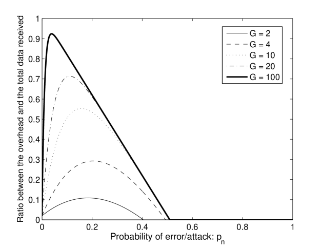
Figure 7: Ratio between the expected overhead and the total data received by a node for generation-based detection with generation size $G$, packet size $1000$ bits, and hash size $o_{g}=\frac{2}{100}(m+l)G$ symbols per generation

V-D Trade-offs and comparisons

In Figures 8 and 9, we compare the three schemes. As mentioned in Section V-B, the expected cost of error correction scheme is linearly proportional to $p_{n}$. Therefore, for large $p_{n}$, this scheme performs badly. However, this simple scheme where a node naively forwards all data it receives outperforms the detection schemes when $p_{n}$ is low ($p_{n}<0.03$). When $p_{n}$ is small, the overhead of detection exceeds the cost introduced by the attackers.

When $p_{n}$ is low, the overhead of our signature is costly, since we are devoting $o_{p}$ symbols per packet to detect an unlikely attack. In such a setting, the generation-based scheme performs well, as it distributes the cost of the hash ($o_{g}$ symbols) over $G$ packets. However, as $p_{n}$ increases, the cost of our signature becomes negligible since the bandwidth wasted by contaminated packets increases; thus, our signature scheme outperforms the generation-based scheme. However, it is important to note that we underestimate the overhead associated with our signature scheme in this paper as we do not take into account the public key distribution cost, which the generation-based scheme does not require. Thus, depending on the public key distribution infrastructure used and the frequency of key renewal, our scheme will incur a higher overhead – resulting in an outward shift in the overhead in Figure 8.

We briefly note the computational cost of implementing these schemes. When using our signature scheme or the generation-based detection scheme, node $n$ does not waste its bandwidth in transmitting contaminated data by dropping a single packet or an entire generation. Furthermore, there is no need of retransmission of the dropped data as the receivers can perform erasure correction on the packets or the generations that have been dropped. It is important to note that for the end-to-end error correction scheme, the receivers need to perform error correction, which is computationally more expensive than erasure correction.

Figure 8: Ratio between the expected overhead and the total data received by a node with $o_{p}=\frac{6}{100}(m+l)$, $o_{g}=\frac{2}{100}(m+l)G$

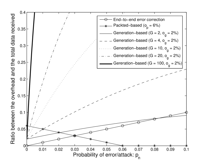
Figure 9: Ratio between the expected overhead and the total data received by a node with $o_{p}=\frac{6}{100}(m+l)$, $o_{g}=\frac{2}{100}(m+l)G$ for $p_{n}\in[0,0.1]$

VI Conclusions

In this paper, we studied the problem of Byzantine attacks in network coded P2P networks. We used randomly evolving graphs to characterize the impact of Byzantine attackers on the receiver’s ability to recover a file. As shown by our analysis, even a small number of attackers can contaminate most of the flow to the receivers. Motivated by this result, we proposed a novel signature scheme for any network using RLNC. The scheme makes use of the linearity of the code, and it can be used to easily check the validity of all received packets. Using this scheme, we can prevent the intermediate nodes from spreading the contamination by allowing nodes to detect contaminated data, drop them, and therefore, only transmit valid data. We emphasize that there is no need of retransmission for the dropped data since the receivers can perform erasure correction, which is computationally cheaper than error correction.

We analyzed the cost and benefit of the signature scheme, and compared it with the end-to-end error correction scheme and the generation-based detection scheme. We showed that the overhead associated with our scheme is low. Furthermore, when the probability of Byzantine attack is high, it is the most bandwidth efficient. However, if the probability of attack is low, generation-based Byzantine detection schemes are more appropriate.

References

- [1] R. Ahlswede, N. Cai, S.-Y. R. Li, and R. W. Yeung, “Network information flow,” IEEE Transactions on Information Theory, vol. 46, pp. 1204–1216, 2000.
- [2] T. Ho, M. Médard, M. Effros, and D. Karger, “The benefits of coding over routing in a randomized setting,” in Proceedings of IEEE ISIT, Kanagawa, Japan, July 2003.
- [3] Z. Li and B. Li, “Network coding: the case of multiple unicast sessions,” in Proceedings of 42nd Annual Allerton Conference on Communication Control and Computing, September 2004.
- [4] D. Lun, M. Médard, and R. Koetter, “Network coding for efficient wireless unicast,” in Proceedings of International Zurich Seminar on Communications, Zurich, Switzerland, February 2006.
- [5] R. Koetter and M. Médard, “An algebraic approach to network coding,” IEEE/ACM Transaction on Networking, vol. 11, pp. 782–795, 2003.
- [6] D. Lun, M. Medard, R. Koetter, and M. Effros, “On coding for reliable communication over packet networks,” Physical Communication, vol. 1, no. 1, pp. 3–20, 2008.
- [7] T. Ho, M. Médard, R. Koetter, M. Effros, J. Shi, and D. R. Karger, “A random linear coding approach to mutlicast,” IEEE Transactions on Information Theory, vol. 52, pp. 4413–4430, 2006.
- [8] S. Acedański, S. Deb, M. Médard, and R. Koetter, “How good is random linear coding based distributed network storage?” in Proceedings of 1st Netcod, Riva del Garda, Italy, April 2005.
- [9] C. Gkantsidis and P. Rodriguez, “Network coding for large scale content distribution,” in Proceedings of IEEE INFOCOM, Miami, FL, March 2005.
- [10] “Bittorrent file sharing protocol,” http://www.BitTorrent.com.
- [11] C. Gkantsidis, J. Miller, and P. Rodriguez, “Comprehensive view of a live network coding p2p system,” in Proceedings of ACM SIGCOMM/USENIX Internet Measurement Conference, Rio de Janeiro, Brazil, October 2006.
- [12] R. Perlman, “Network layer protocols with byzantine robustness,” Ph.D. dissertation, Massachusetts Institute of Technology, Cambridge, MA, October 1988.
- [13] M. Castro and B. Liskov, “Practical byzantine fault tolerance,” in Symposium on Operating Systems Design and Implementation (OSDI), February 1999.
- [14] L. Lamport, R. Shostak, and M. Pease, “The byzantine generals problem,” ACM Transactions on Programming Languages and Systems, vol. 4, pp. 382–401, 1982.
- [15] S. Jaggi, M. Langberg, S. Katti, T. Ho, D. Katabi, and M. Médard, “Resilient network coding in the presence of byzantine adversaries,” in Proceedings of IEEE INFOCOM, March 2007, pp. 616 – 624.
- [16] C. Gkantsidis and P. Rodriguez, “Cooperative security for network coding file distribution,” in Proceedings of IEEE INFOCOM, April 2006.
- [17] A. Barabási and R. Albert, “Emergence of Scaling in Random Networks,” Science, vol. 286, no. 5439, p. 509, 1999.
- [18] L. A. Adamic, R. M. Lukose, A. R. Puniyani, and B. A. Huberman, “Search in power-law networks,” Phys. Rev. E, vol. 64, no. 4, p. 046135, September 2001.
- [19] R. Pastor-Satorras and A. Vespignani, “Epidemic spreading in scale-free networks,” Phys. Rev. Lett., vol. 86, no. 14, pp. 3200–3203, Apr 2001.
- [20] R. M. May and A. L. Lloyd, “Infection dynamics on scale-free networks,” Phys. Rev. E, vol. 64, no. 6, p. 066112, Nov 2001.
- [21] A. G. Dimakis, P. B. Godfrey, M. J. Wainwright, and K. Ramchandran, “Network coding for distributed storage systems,” in Proceedings of IEEE INFOCOM, Anchorage, Alaska, May 2007.
- [22] R. W. Yeung and N. Cai, “Network error correction,” Communications in Information and Systems, no. 1, pp. 19–54, 2006.
- [23] R. Koetter and F. Kschischang, “Coding for errors and erasures in random network coding,” IEEE Transactions on Information Theory, vol. 54, pp. 3579–3591, 2008.
- [24] D. Silva and F. Kschischang, “Adversarial error correction for network coding: Models and metrics,” in Proceedings of Annual Allerton Conf. on Commun., Control, and Computing, Monticello, IL, September 2008.
- [25] T. Ho, B. Leong, R. Koetter, M. Médard, and M. Effros, “Byzantine modification detection in multicast networks using randomized network coding,” in Proceedings of IEEE ISIT, June 2004.
- [26] M. Krohn, M. Freedman, and D. Mazières, “On-the-fly verification of rateless erasure codes for efficient content distribution,” in Proceedings of IEEE Symposium on Security and Privacy, May 2004.
- [27] Z. Yu, Y. Wei, B. Ramkumar, and Y. Guan, “An efficient signature-based scheme for securing network coding against pollution attacks,” in Proceedings of IEEE INFOCOM, Pheonix, AZ, April 2008.
- [28] D. Charles, K. Jain, and K. Lauter, “Signatures for network coding,” in Proceedings of Conference on Information Sciences and Systems, March 2006.
- [29] National Institute of Standards and Technology, “Digital signature standard (DSS),” FIBS PUB 186-2, 2000.
- [30] D. Boneh and M. Franklin, “An efficient public key traitor tracing scheme,” in Lecture Notes in Computer Science, vol. 1666. Springer-Verlag, 1999, pp. 338–353.