Optical wave turbulence and the condensation of light

Abstract

In an optical experiment, we report a wave turbulence regime that, starting with weakly nonlinear waves with randomized phases, shows an inverse cascade of photons towards the lowest wavenumbers. We show that the cascade is induced by a six-wave resonant interaction process and is characterized by increasing nonlinearity. At low wavenumbers the nonlinearity becomes strong and leads to modulational instability developing into solitons, whose number is decreasing further along the beam.

The idea to create the state of optical wave turbulence (OWT) has excited the minds of scientists for over thirty years, and it was a subject of a rather large number of theoretical papers OT ; OT2 ; OT3 ; OT4 ; NO . Indeed there are some far reaching fluid analogies in the dynamics of nonlinear light, for example vortex-like solutions OV ; OV2 , shock waves Fleischer and weakly interacting random waves whose dynamics and statistics has similarities to the system of random waves on water surface zf ; zlf . OWT was theoretically predicted to exhibit dual cascade properties similar to 2D fluid turbulence, namely the energy cascading directly, from low to high frequencies, and the photons cascading inversely, toward the low energy states zlf ; OT ; OT2 ; OT3 ; OT4 . When the nonlinearity is small, OWT can be described by the theory of weak turbulence (WT) zlf which possesses classical attributes of the general turbulence theory, particularly predictions of the Kolmogorov-like cascade states, which in the WT context are called Kolmogorov-Zakharov (KZ) spectra. It appears that OWT has two KZ states: one describing the direct energy cascade from large to small scales, and the second one - an inverse cascade of wave action toward larger scales. The inverse cascade is particularly interesting because in the optics context it means condensation of photons. Furthermore, it was theoretically predicted, and numerically observed in some WT systems, that in the course of the inverse cascade the nonlinearity will grow, which will eventually lead to the breakdown of the WT description at low wavenumbers and to the formation of coherent structures OT ; OT3 ; NO ; MMT97 ; CMMT01 ; DPZ04 . In optics, these can be solitons or collapses for focusing nonlinearity or a quasi-uniform condensate and vortices for the defocusing case.

The final thermalized state was studied extensively theoretically in various settings for non-integrable Hamiltonian systems starting with the pioneering paper by Zakharov et al ZPSY88 , see also RN01 ; RN03 ; BKKMMP09 ; ET06 ; JJ00 ; RCK00 ; JTZ00 ; PPM08 ; PLJP06 ; PY85 . The final state with a single soliton and small-scale noise was interpreted as a statistical attractor, and an analogy was pointed out to the over-saturated vapor system, where the solitons are similar to droplets and the random waves are like molecules PY85 . There, small droplets evaporate while the big ones gain size from the free molecules, resulting in the decrease in the number of droplets. In our work we put emphasis on turbulence, i.e. on a transient non-equilibrium process leading to thermalization rather than the thermal equilibrium itself.

We report the first experimental evidence of OWT: starting with weakly nonlinear incoherent waves we observe an inverse cascade of the photons to lower wavenumbers and growth of the nonlinearity leading to the formation of multiple coherent solitons, which further merge into a single strong soliton. This corresponds to Bose-Einstein condensation (BEC) of photons, which is an optical analogue of atomic BEC reported in bec ; bec2 .

The motion of photons to different energy levels (and toward the lowest one corresponding to condensation) can be achieved via nonlinear interactions of photons, provided for example by the Kerr effect. The problem, however, is that the nonlinearity is usually very weak and it is an experimental challenge to make it overpower the dissipation. In our view this was the main obstacle with the photon condensation setup in a 2D Fabry-Perot cavity theoretically suggested in chiao .

The key feature in our setup is that we traded one spatial dimension for a “time axis”, namely we considered a time independent 2D light field where the principal direction of the light propagation plays the role of “time”. This allowed us to use a nematic liquid crystal, which provides a high level and tunable optical nonlinearity Zeldovich ; Khoo . The slow relaxation time of the reorientational dynamics is not a restriction in our setup because our system is steady in time. Similar experiments were first reported in Libchaber , where it was shown that a beam propagating inside a nematic layer undergoes a strong self-focusing effect followed by filamentation, soliton formation, when the light intensity is increased. More recently, a renewed interest in the same setup has led to further studies on the optical solitons and modulational instability regimes Assanto ; Peccianti ; Conti . However, all these experiments have in common a large value of the input intensity, of the order of $10^{3}$ $W/cm^{2}$, therefore the optical nonlinearity is rather high and, as soon as the beam enter the liquid crystal, the soliton or modulational instability regimes appear immediately, bypassing the WT regime.

In our experiment, we fix a much lower input intensity, of the order of $10^{-1}$ $W/cm^{2}$, and, for the first time, we show that, before the modulational instability and the soliton formation, corresponding to the breakdown of the weak nonlinearity, there is a WT regime characterized by an inverse cascade of the photon number. Besides the weak nonlinearity, to allow for the wave-mixing and the inverse cascade development, we also need to prepare a proper initial condition: we start with weakly nonlinear incoherent waves, characterized by high wavenumbers and random phases.

The 1D system is rather different from the 2D and 3D systems considered theoretically before, and in this paper, for the first time, we present a theory of 1D OWT, which involves coexisting random waves (interacting via a six-wave process) and solitons (to which the random waves condense). We complement our study with the numerical simulation of the dynamical equation, and we observe that the theory, numerics and experiment are consistent and complementary with each other, giving a rather complete description of the 1D OWT phenomenon.

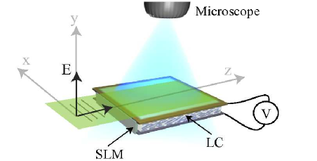
Figure 1: (color online). Experimental setup: a laminar shaped input beam propagates inside the liquid crystal (LC) layer; random space modulations are imposed at the entrance of the cell by means of a spatial light modulator (SLM).

The experimental apparatus is shown in Fig. 1. It consists of a laminar shaped beam propagating inside a nematic liquid crystal (LC) layer. Before entering the cell, the beam passes through a spatial light modulator (SLM) that, through suitable intensity masks, modulates the input profile for injecting random phased fields with large wavenumbers. The LC cell is made by sandwiching a nematic layer (E48) of thickness $d=50$ $\mu m$ between two $20\times 30$ $mm^{2}$ glass windows. On the interior, the glass walls are coated with Indium-Tin-Oxide (ITO) transparent electrodes. We have pre-treated the ITO surfaces in order to align all the molecules parallel to the confining walls (nematic director along $\hat{z}$). The LC layer behaves as a positive uniaxial medium, with $n_{e}=1.7$ the extraordinary and $n_{o}=1.5$, the ordinary refractive indices Khoo . LC molecules tend to turn more along the applied field and the refractive index $n(\theta)$ follows the distribution of the tilt angle. We apply a $1$ $kHz$ electric field with rms voltage $V_{0}=2.5$ $V$ so that the molecular director is preset to an average tilt $\theta$. When a linearly polarized beam is injected into the cell, the LC molecules reorient towards the direction of the input polarization. The input light comes from a diode pumped solid state laser, $\lambda=473$ $nm$, linearly polarized along $\hat{y}$ and shaped as a thin laminar Gaussian beam of $30$ $\mu m$ thickness, $1.8$ $mm$ width. The total power was $200$ $\mu W$, corresponding to an input intensity of $370$ $mW/cm^{2}$, which is low enough to ensure the weakly nonlinear regime. The beam evolution inside the cell is monitored with an optical microscope and a CCD camera.

Theoretically, the beam evolution is described by a propagation equation for the input beam coupled to a relaxation equation for the LC dynamics

$$2iq{\partial\psi\over\partial z}+{\partial^{2}\psi\over\partial x^{2}}+k_{0}^{2}n_{a}^{2}a\psi = 0,$$ (1)

$${\partial^{2}a\over\partial x^{2}}-{1\over l_{\xi}^{2}}a+{\varepsilon_{0}n_{a}^{2}\over 4K}|\psi|^{2} = 0,$$ (2)

where $\psi(x,z)$ is the complex amplitude of the input beam propagating along “time axis” $\hat{z}$, $x$ the coordinate across the beam, $a(x,z)$ the liquid crystal reorientation angle, $n_{a}=n_{e}-n_{o}$ the birefringence of the LC, $k_{0}$ the optical wavenumber, $\varepsilon_{0}$ the vacuum permittivity and $l_{\xi}=\left(\pi K/2\Delta\varepsilon\right)^{1/2}(d/V_{0})$ the electrical coherence length of the LC DeGennes , with $K$ the elastic constant, $q^{2}=k_{0}^{2}\left(n_{o}^{2}+n_{a}^{2}/2\right)$ and $\Delta\varepsilon$ the dielectric anisotropy. Note that $l_{\xi}$ fixes the typical dissipation scale, limiting the extent of the inertial range in which the WT cascade develops. In other contexts, see e.g. Assanto ; Peccianti ; Conti , such a spatial diffusion of the molecular deformation has been denoted as a nonlocal effect. In our experiment, for $V_{0}=2.5$ $V$ we have $l_{\xi}=9$ $\mu m$. The experimental setup corresponds to the long-wave regime, $kl_{\xi}\ll 1$, where $k$ is the typical wavenumber inside the range of the inverse cascade. Therefore, in this paper we consider the limit $kl_{\xi}\ll 1$ of Eqs. (1) and (2), which enables us to form a single equation for the input beam us :

$$2iq{\partial\psi\over\partial z}=-{\partial^{2}\psi\over\partial x^{2}}-{\varepsilon_{0}n_{a}^{4}l_{\xi}^{2}k_{0}^{2}\over 4K}\left(\psi|\psi|^{2}+l_{\xi}^{2}\psi{\partial^{2}|\psi|^{2}\over\partial x^{2}}\right)=\frac{\delta H}{\delta\psi^{*}}.$$ (3)

Eq. (3) conserves the energy

$$H=\int{\left|{\partial\psi\over\partial x}\right|^{2}-{\varepsilon_{0}n_{a}^{4}l_{\xi}^{2}k^{2}_{0}\over 8K}\left[|\psi|^{4}-l_{\xi}^{2}\left({\partial|\psi|^{2}\over\partial x}\right)^{2}\right]}dx,$$ (4)

and the number of photons, $N=\int|\psi|^{2}\,dx.$ In the limit ${\varepsilon_{0}n_{a}^{4}l_{\xi}^{2}k_{0}^{2}/2K}\to 0$, Eq. (3) becomes the linear Schrödinger equation and has linear wave solutions $\psi(x,z)\sim a_{k}\exp(-i\omega_{k}z+ikx)$ with “frequencies” $\omega=k^{2}$ and constant complex amplitudes $a_{k}$. For weak nonlinearity the amplitude $a_{k}$ become weakly dependent on “time” $z$. Note that the leading nonlinear term cannot generate a cascade in $k$ because it corresponds to an integrable 1D Nonlinear Schrödinger equation. Thus, we retain the sub-leading term and apply the WT theory, which allows us to describe weakly nonlinear waves with random phases of $a_{k}$. To apply the WT theory, we also need to verify that the linear dynamics dominate in the system. The ratio of the linear term and the leading nonlinear term of Eq. (3) is

$$J=\frac{4Kk^{2}}{\epsilon_{0}n_{a}^{4}k_{0}^{2}l_{\xi}^{2}I},$$ (5)

where $I$ is the input intensity. For $I=370$ $mW/cm^{2}$ we have $J\simeq 100$, which ensures the validity of the WT approach.

For the wave action spectrum $n_{k}=\langle a_{k}a_{k}^{*}\rangle$ (the averaging is over the random phases), the WT approach yields to the following kinetic equation us ,

$${\partial n_{k}\over\partial z} = A\int f_{k12345}\;\delta(k+k_{1}+k_{2}-k_{3}-k_{4}-k_{5})$$ (6)

$$\times\delta(\omega_{k}+\omega_{1}+\omega_{2}-\omega_{3}-\omega_{4}-\omega_{5})dk_{1}dk_{2}dk_{3}dk_{4}dk_{5},$$

with $f_{k12345}=n_{k}n_{1}n_{2}n_{3}n_{4}n_{5}({1\over n_{k}}+{1\over n_{1}}+{1\over n_{2}}-{1\over n_{3}}-{1\over n_{4}}-{1\over n_{5}})$ and $A={9\pi k^{8}_{0}n_{a}^{16}l_{\xi}^{12}\epsilon_{0}^{4}/2048K^{4}}$.

The kinetic equation has important exact power law solutions $n_{k}=C|k|^{-\nu}$ where $C$ and $\nu$ are constants. In particular, $\nu=0$ and $\nu=2$ correspond to thermodynamic equilibria with equipartitions of the particle density and the energy respectively. In addition, there are KZ power law solutions corresponding to a direct energy cascade from low to high $k$’s,

$$n_{k}=C|k|^{-1},$$ (7)

and an inverse wave action cascade from high to low $k$’s,

$$n_{k}=C|k|^{-3/5}.$$ (8)

Note, that a kinetic equation can be derived directly from Eqs. (1) and (2) without the assumption of $kl_{\xi}\ll 1$. We will consider the general case, including the short-wave limit of Eqs. (1) and (2) in an extended publication us .

Here, we concentrate on the inverse cascade. The inverse cascade spectrum is of a finite capacity type, in a sense that only a finite amount of the cascading invariant (wave action in this case) is needed to fill the infinite inertial range. (Indeed, the integral of $n_{k}\sim k^{-3/5}$ converges at $k=0$). In these cases the turbulent systems have a long transient (on its way to the final thermal equilibrium state) in which the scaling is of the KZ type. This is because the initial condition serves as a huge reservoir of the cascading invariant. Note that the situation here is not specific for WT only and it is valid generally for turbulence. For example, it is valid for Navier-Stokes turbulence, i.e. the Kolmogorov-Obukhov spectrum, which is also finite capacity.

To set up the inverse cascade, we have injected photons at small spatial scales with random phases. This is made by creating through the SLM a random distribution of diffusing spots with the average size $\sim 35$ $\mu m$. The numerical initial condition is more idealized and strictly localized at a small-scale range: we excite five wavenumbers with constant amplitude around $|k_{f}|\sim 1.5\times 10^{2}$ $mm^{-1}$, with the phase of $\psi_{k}$ being random and independent at each $k$. Moreover, we apply a Gaussian filter in physical space to achieve a beam profile comparable to that of the experiment. Applicability of the WT approach for the numerical simulation is verified by the calculation of parameter $J$, which agrees with the experiment and is of the order of $J\simeq 100$. Experimentally, we measure the light intensity $I(x,z)=|\psi|^{2}$ and not the phases of $\psi$ and, therefore, the spectrum $n_{k}$ is not directly accessible. Instead, we measure the spectrum of intensity $N(k,z)=|I_{k}(z)|^{2}$. The scaling for $N_{k}$ in the inverse cascade state is easy to obtain from the wave action spectrum (8) and the random phase condition; this gives

$$N_{k}\sim|k|^{-1/5}.$$ (9)

Experimental and numerical spectra of the light intensity are shown in Figs. 2 and 3 respectively. In both cases one can see an inverse cascade excitation of the lower $k$ states, and good agreement with the WT prediction of the intensity spectrum (9).

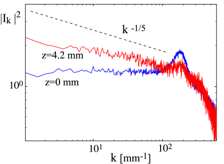
Figure 2: (color online). Experimental spectrum of the light intensity, $N_{k}=|I_{k}|^{2}$ at two different distances $z$.

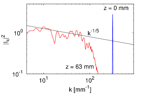
Figure 3: (color online). Numerical spectrum of the light intensity, $N_{k}=|I_{k}|^{2}$ at two different distances $z$. Averaging is taken over a small finite time window and over ten realizations.

Closeness of Eq. (3) to integrability means that we should expect not only random waves but also soliton-like coherent structures. In the inverse cascade setup the solitons appear naturally. Indeed, the WT description (Eq. (6)) breaks down when the inverse cascade reaches some low $k$’s us . Modulational instability develops at these scales, which results in filamentation of light and its condensation into coherent structures - solitons.

Verification of the long-wave limit $kl_{\xi}\ll 1$ and deviation from integrability is checked by considering the ratio of the two nonlinear terms in Eq. (3), which is estimated in Fourier space as $R\sim k^{2}l_{\xi}^{2}$. We find from Figs. 2 and 3 that the inverse cascade is approximately in the region $k\sim 10^{4}-10^{5}$ $m^{-1}$ giving an estimation of $R\sim 10^{-2}-1$. Note, that if $R$ is too small, then we are close to a purely integrable system, which would be dominated by solitons and lack cascade dynamics, and if too high then our model breaks down.

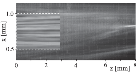
Figure 4: Experimental results for intensity distribution $I(x,z)$. Area marked by the dashed line is shown at a higher resolution (using a larger magnification objectif).

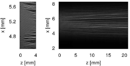
Figure 5: Numerical results for intensity distribution $I(x,z)$. The frame on the left is a magnified section of the initial propagation of the beam.

Example zooms of the intensity distribution $I(x,z)$ showing the beam evolution during propagation in the experiment and in the numerics are displayed in Fig. 4 and Fig.5 respectively. In the high resolution insets on Figs. 4 and 5 one can visually observe that the typical scale increases along the beam which corresponds to an inverse cascade process. Furthermore, in both Fig. 4 and Fig. 5 one can see the formation of coherent solitons out of the random initial field, with the overall number of solitons reducing as the beam propagates. Experimentally, the condensation into one dominant soliton is well revealed by the linear intensity profiles $I(x)$ taken at different propagation distances, as shown in Fig. 6 for $z=0.3$, $4.5$ and $7.5$ $mm$. Note that the amplitude of the final dominant soliton is three orders of magnitude larger than the amplitude of the initial periodic modulation.

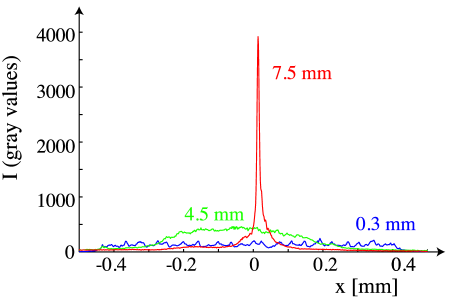
Figure 6: (color online) Linear intensity profiles $I(x)$ taken at different propagation distances, $z=0.3$, $4.5$ and $7.5$ $mm$.

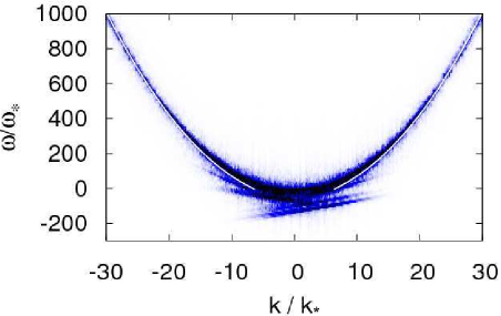
Figure 7: (color online). The $k-\omega$ spectrum of the wave field at $z=2.1$ $m$. $\omega_{*}=1/256ql^{2}_{\xi}$ and $k_{*}=1/\sqrt{128}l_{\xi}$. The Bogoliubov dispersion relation is shown by the solid line.

We perform two numerical simulations, one with a domain comparable with the experiment (Figs. 5 and  3) and another with a lower intensity initial condition over a longer propagation distance $z$, to allow us to clearly distinguish between the WT inverse cascade and MI (Fig. 7). Deviations from integrability result in the interactions of the solitons with each other and with the random waves, which lead to changes of the soliton strengths. Both the experimental and the numerical results in Fig. 4 and Fig. 5 indicate that solitons gradually merge, reducing the total number. The observed increase of the scale and formation of coherent structures represent the condensation of light.

Separating the random wave and the coherent soliton components can be done via performing an additional Fourier transform with respect to “time” $z$ over a finite $z$-window determined by the frequency scale NO . Such numerically obtained $(k,\omega)$-plot is shown in Fig. 7. There, the incoherent wave component is distributed around the wave dispersion relation, which is Bogoliubov-modified by the condensate us and is shown by a solid line in Fig. 7 (the line ends at a finite $k$ below which $\omega$ becomes imaginary corresponding to modulational instability). This distribution is narrow for large $k$ which corresponds to weak nonlinearity, and it gets wider toward low $k$, which coincides with the growth of the nonlinearity and the breakdown of the WT applicability conditions. For these low $k$ values one can see pieces of slanted lines (under the dispersion curve) each corresponding to a coherent soliton, whose speed is equal to the slope.

In conclusion, we have presented the first experimental implementation, numerical simulations and theory of 1D OWT. We observe an inverse cascade of photons toward the states with lower frequencies with a respective KZ spectrum predicted by the WT theory. The inverse cascade is accompanied by increasing nonlinearity and the eventual breakdown of WT, leading to the light condensing into coherent structures - solitons.

This work has been partially supported by the Royal Society’s International Joint Project grant, and by the ANR-07-BLAN-0246-03, turbonde. U.B. and S.R. acknowledge helpful discussion with Gaetano Assanto and Armando Piccardi.

References

- (1) S. Dyachenko, A.C. Newell, A. Pushkarev, and V.E. Zakharov, “Optical turbulence: weak turbulence, condensates and collapsing filaments in the nonlinear Schrödinger equation,” Physica D 57, 96-160 (1992).
- (2) S.L. Musher, A.M. Rubenchik, and V.E. Zakharov, “Hamiltonian approach to the description of nonlinear plasma phenomena,” Phys. Rep. 129, 285-366 (1985).
- (3) S. Nazarenko, and V. Zakharov, “Dynamics of the Bose-Einstein condensation,” Physica D 201, 203-211 (2005).
- (4) C. Connaughton, C. Josserand, A. Picozzi, Y. Pomeau, and S. Rica, “Condensation of classical nonlinear waves,” Phys. Rev. Lett. 95, 263901 (2005).
- (5) S. Nazarenko, and M. Onorato, “Wave turbulence and vortices in Bose-Einstein condensation,” Physica D Nonlinear Phenomena 219, 1 (2006).
- (6) F.T. Arecchi, G. Giacomelli, P.L. Ramazza, and S. Residori, “Vortices and defect statistics in two-dimensional optical chaos,” Phys. Rev. Lett. 67, 3749 (1991).
- (7) G. A. Swartzlander Jr. and C. T. Law, “Optical vortex solitons observed in Kerr nonlinear media,” Phys. Rev. Lett. 69, 2503 (1992).
- (8) C. Barsi, W. Wan, C. Sun, and J.W. Fleischer, “Dispersive shock waves with nonlocal nonlinearity,” Opt. Lett. 32, 2930 (2007).
- (9) V.E. Zakharov, and N.N. Filonenko, “The energy spectrum for stochastic oscillations of a fluid surface,” Sov. Phys. Dokl. 11, 881 (1967).
- (10) V.E. Zakharov, V.S. Lvov, and G. Falkovich, Kolmogorov Spectra of Turbulence, (Springer-Verlag, 1992).
- (11) F. Dias, A. Pushkarev, V. Zakharov, “One-dimensional wave turbulence”, Physics Reports, 398, 1-65 (2004).
- (12) A.J. Majda, D.W. McLaughlin, E.G. Tabak, “A one-dimensional model for dispersive wave turbulence”, J. Nonlinear Sci. 6, 9 44 (1997).
- (13) D. Cai, A.J. Majda, D.W. McLaughlin, E.G. Tabak, “Dispersive wave turbulence in one dimension”, Physica D, 152-153, 551-572, (2001).
- (14) V.E. Zakharov, A.N. Pushkarev, V.F. Shvets and V.V. Yan’kov, “Soliton turbulence,” JETP Lett. 48, No. 2, 83-87 (1988).
- (15) S. Pitois, S. Lagrange, H.R. Jauslin and A. Picozzi, “Velocity locking of inocherent nonlinear wave packets,” Phys. Rev. Lett. 97, 033902 (2006).
- (16) A. Picozzi, S. Pitois and G Millot, “Spectral incoherent solitons: a localized soliton behavior in the frequency domain”, Phys. Rev. Lett. 101, 093901 (2008).
- (17) R. Jordan, B. Turkington and C.L. Zirbel, “A mean-field statistical theory for the nonlinear Schrödinger equation,” Physica D, 137, 353-378 (2000).
- (18) K.Ø. Rasmussen, T. Cretegny and P.G. Kevrekidis, “Statistical mechanics of a discrete nonlinear system,” Phys. Rev. Lett. 84, 17 (2000).
- (19) R. Jordan and C. Josserand, “Self-organization in nonlinear wave turbulence,” Phys. Rev. E, 61, 1 (2000).
- (20) A. Eisner and B. Turkington, “Nonequilibrium statistical behavior of nonlinear Schrödinger equations,” Physica D, 213, 85-97 (2006).
- (21) B. Barviau, B. Kibler, A. Kudlinski, A. Mussot, H. Millot and A. Picozzi, “Experimental signature of optical wave thermalization through supercontinuum generation in photonic crystal fiber,” Opt. Express 17, 7392 (2009).
- (22) B. Rumpf and A.C. Newell, “Localization and coherence in nonintegrable systems,” Physica D, 184, 162-191 (2003).
- (23) B. Rumpf and A.C. Newell, “Coherent structures and entropy in constrained, modulationally unstable, nonintegrable systems,” Phys. Rev. Lett. 87, 5 (2001).
- (24) V.I. Petviashvili and V.V. Yan’kov, “Solitons and Turbulence,” Reviews of Plasma Physics, 14, (1987).
- (25) M.H. Anderson, J.R. Ensher, M.R. Matthews, C.E. Wieman, and E.A. Cornell, “Observation of Bose-Einstein condensation in a dilute atomic vapor,” Science 269, 198-201 (1995).
- (26) L.P. Pitaevskii, and S. Stringari, Bose-Einstein Condensation, (Clarendon Press, Oxford, 2003).
- (27) R.Y. Chiao, and J. Boyce, “Bogoliubov dispersion relation and the possibility of superfluidity for weakly interacting photons in a two-dimensional photon fluid,” Phys. Rev. A 60, 4114-4121 (1999).
- (28) N.V. Tabiryan, A.V. Sukhov and V.Y. Zeldovich, “The orientational optical nonlinearity of liquid crystals,” Mol. Cryst. Liq. Cryst., 136, 1 (1986).
- (29) I.C. Khoo, Liquid Crystals: Physical Properties and Nonlinear Optical Phenomena (Wiley, New York, 1995).
- (30) E. Braun, L.P. Faucheux, and A. Libchaber, “Strong self-focusing in nematic liquid crystals,” Phys. Rev. A 48, 611-622 (1993).
- (31) M. Peccianti, C. Conti, G. Assanto, A. De Luca, and C. Umeton, “Routing of anisotropic spatial solitons and modulational instability in liquid crystals,” Nature 432, 733 (2004).
- (32) M. Peccianti, C. Conti, and G. Assanto, “Optical modulational instability in a nonlocal medium,” Phys. Rev. E 68, 025602 (2003).
- (33) C. Conti, M. Peccianti, and G. Assanto, “Complex dynamics and configurational entropy of spatial optical solitons in nonlocal media,” Opt. Lett. 31, 2030 (2006).
- (34) P.G. De Gennes, and J. Prost, The Physics of Liquid Crystals, (Oxford Science Publications, Clarendon Press, second edition, 1993).
- (35) U. Bortolozzo, J. Laurie, S. Nazarenko and S. Residori are preparing a larger manuscript to be called “One-dimensional optical wave turbulence.”