Zonal flows and long-distance correlations during the formation of the edge shear layer in the TJ-II stellarator

Abstract

A theoretical interpretation is given for the observed long-distance correlations in potential fluctuations in TJ-II. The value of the correlation increases above the critical point of the transition for the emergence of the plasma edge shear flow layer. Mean (i.e. surface averaged, zero-frequency) sheared flows cannot account for the experimental results. A model consisting of four envelope equations for the fluctuation level, the mean flow shear, the zonal flow amplitude shear, and the averaged pressure gradient is proposed. It is shown that the presence of zonal flows is essential to reproduce the main features of the experimental observations.

I Introduction

Transport barrier formation is mostly caused by the emergence of a radial electric field shear Burrell (1997); Terry (2000); Burrell (2006). This radial electric field may be induced by poloidal flows and/or a gradient in the pressure, apart from the direct particle losses.

A simple model for barrier formation and transition to a high confinement regime that was solely based on the poloidal flow shear was proposed in Ref. Diamond et al. (1994). In this model a mean sheared flow is amplified by the Reynolds stress Hasegawa and Wakatani (1987); Carreras et al. (1991); Diamond and Kim (1991) and turbulence is suppressed by shearing Biglari et al. (1990). The combination between those two effects allows having two possible types of states. On the one hand, states with vanishing flow shear and high turbulence level (low confinement). On the other hand, above a critical threshold, states with non-zero flow shear and reduced turbulence fluctuations (improved confinement). The transition between these two types of states is a continuous bifurcation.

In Ref. Carreras et al. (1994) the model was extended by incorporating the pressure gradient component of the radial electric field. This extended model shows the existence of two critical points, the first being the same as in the previous model. The second transition, happening at higher density and temperature, is a discontinuous transition to a zero fluctuation state where the radial electric field is only due to the pressure gradient. Experiments have shown E. J. Doyle, P. Gohil, R. J. Groebner, T. Lehecka, N. C. Luhmann, M. A. Mahdavi, T. H. Osborne, W. A. Peebles, and R. Philipona that the L to H transition Wagner et al. (1982) leads to a high confinement state with the radial electric field shear dominated by the pressure gradient. That is why the second transition in this model has been associated to the L to H transition.

Recently and in experiments carried out in the TJ-II stellarator, the first transition (linked to the generation of the poloidal flow) has been identified Pedrosa et al. (2005); Carreras et al. (2006); M. A. Pedrosa, B. A. Carreras, C. Hidalgo, C. Silva, M. Hron, L. García, J. A. Alonso, I. Calvo, J. L. de Pablos, and J. Stöckel (2007); Delgado et al. (2009) with the emergence of the plasma edge shear flow layer Ritz et al. (1984); J. A. Wooton, B. A. Carreras, H. Matsumoto, K. McGuire, W. A. Peebles, C. P. Ritz, P. W. Terry, and S. J. Zweben (1990).

New experimental results Pedrosa et al. (2008) report the existence of long-range potential correlations in the toroidal direction. Two probes are set toroidally separated and not in the same field line. In addition, consider the intersection point of the field line going through the first probe with the plane of the second probe. The distance between this intersection point and the second probe is larger than a poloidal correlation length of the high-$k$ turbulence. These correlations are observed during the transition leading to the formation of the plasma edge shear flow layer in TJ-II. The observed correlations correspond to (non-zero) frequencies below 30 kHz and thus they cannot be explained by mean (i.e. surface averaged, zero-frequency) sheared flows. In the present work we aim to show that the experimental findings of Ref. Pedrosa et al. (2008) can be understood in the framework of simple transition models if one appropriately incorporates the contribution of zonal flows Diamond et al. (2005). Here we use the term zonal flow in the sense of low frequency fluctuating flows with $k_{\varphi}=0$ and small but non-zero $k_{\theta}$. A transition model including zonal flows was proposed in Ref. Kim and Diamond (2003), which we slightly extend here in order to interpret the TJ-II results. The structure of the model equations is based on quasilinear calculations from pressure-gradient-driven turbulence Carreras et al. (1993). In this paper, we use a phenomenological approach, determining the main parameters of the model from the experimental results. We will see that the model is able to capture the essential features of the experimental observations.

In Section II we present the transition model incorporating the effect of zonal flows. In Section III a comparison with the experimental data is performed. Conclusions are collected in Section IV.

II The transition model

The model presented in this section is an extension of the one used in Ref. Carreras et al. (2006) to discuss the emergence of the plasma edge shear flow layer. This is a model formulated at a radial point. The dynamical variables are the fluctuation level envelope ${\cal E}:=\langle(\tilde{n}/n_{0})^{2}\rangle^{1/2}$, the mean flow shear ${\cal V}:=\partial_{r}\langle V_{\theta}\rangle$, the zonal flow amplitude shear, ${\cal V}_{\rm{ZF}}:=\partial_{r}\langle V_{\theta\rm{ZF}}\rangle$, and (minus) the normalized average pressure gradient ${\cal N}:=-a\partial_{r}\langle p\rangle/\langle p\rangle(0)$. Here $a$ is the minor radius of the torus, $\langle\cdot\rangle$ stands for the average over angle coordinates, and $r=0$ corresponds to the magnetic axis. The equations of the model are

$$\frac{\mbox{d}{\cal E}}{\mbox{d}\tau}=\gamma_{0}{\cal N}^{2/3}{\cal E}-\alpha_{1}{\cal N}^{-1/2}{\cal E}^{2}-\alpha_{2}{\cal E}{\cal N}^{-1/3}({\cal V}^{2}+{\cal V}_{\rm{ZF}}^{2}),$$ (1a)

$$\frac{\mbox{d}{\cal V}}{\mbox{d}\tau}=\bar{a}_{1}{\cal N}^{-4/3}{\cal E}^{2}{\cal V}+\bar{a}_{2}{\cal N}^{-2/3}{\cal V}_{\rm{ZF}}^{2}{\cal V}-\bar{b}{\cal V},$$ (1b)

$$\frac{\mbox{d}{\cal V}_{\rm{ZF}}}{\mbox{d}\tau}=\frac{\bar{a}_{1}}{1+\frac{\alpha_{2}}{\gamma_{0}}{\cal N}^{-1}{\cal V}^{2}}{\cal N}^{-4/3}{\cal E}^{2}{\cal V}_{\rm{ZF}}+\bar{a}_{3}{\cal N}^{-4/3}{\cal E}^{2}{\cal V}-\bar{b}{\cal V}_{\rm{ZF}},$$ (1c)

$$\frac{\mbox{d}{\cal N}}{\mbox{d}\tau}=\bar{\Gamma}-\bar{D}{\cal E}{\cal N}.$$ (1d)

The structure of these equations is based on a quasilinear approximation of resistive pressure-gradient driven turbulence (the resistive interchange mode, due to bad magnetic field line curvature, is assumed to be the basic instability at the edge of TJ-II). The linear eigenfunctions and the dependence of the linear growth rates on $\cal N$ were computed in Carreras et al. (1993). In particular, we have used a fluid approach to calculate the poloidal velocity shear and the sheared radial electric field. The reason is that the TJ-II plasma edge, $r/a>0.8$, is in the collisional regime. We would like to point out that for the range of powers and densities in TJ-II considered here, neoclassical theory is only applicable to the inner region, $r/a<0.25$. In addition, it has been shown Castejón et al. (2002) that in this regime the ambipolar radial electric field in TJ-II is small and shearless for $r>5$ cm and that the electron root Hastings et al. (1985) is the only accessible root. Therefore, in the edge region the fluid formulation seems to be adequate for the studies to be carried out in this paper.

The first term on the right-hand side of Eq. (1a) corresponds to the linear instability generation of turbulence, the second to the non-linear saturation of the instability, and the two last terms to the supression of turbulence by sheared mean and zonal flows. The first and second terms on the right-hand side of Eq. (1b) represent the generation of mean sheared flow by Reynolds stress, and the third one is the collisional damping term (analogous to the last term on the right-hand side of Eq. (1c)). The two first terms on the right-hand side of Eq. (1c) give the generation of zonal flow by Reynolds stress; in the first term the factor $(1+\alpha_{2}{\cal N}^{-1}{\cal V}^{2}/\gamma_{0})^{-1}$ corresponds to the effect of zonal flow supression by a mean sheared flow. Finally, in Eq. (1d), $\bar{D}{\cal E}$ is the anomalous particle diffusivity, and $\bar{\Gamma}$ the normalized incremental particle flux, the control parameter of the model. Diamagnetic effects in the momentum balance equation have been neglected because we consider small values of $\bar{\Gamma}$.

In terms of dimensionless variables,

$$t=\gamma_{0}\tau,\ \ E=\frac{\alpha_{1}}{\gamma_{0}}{\cal E},\ \ V=\sqrt{\frac{\alpha_{2}}{\gamma_{0}}}{\cal V},\ \ V_{\rm{ZF}}=\sqrt{\frac{\alpha_{2}}{\gamma_{0}}}{\cal V}_{\rm{ZF}},\ \ N={\cal N},$$ (2)

the equations read:

$$\frac{\mbox{d}E}{\mbox{d}t}=N^{2/3}E-N^{-1/2}E^{2}-N^{-1/3}E(V^{2}+V_{\rm{ZF}}^{2}),$$ (3a)

$$\frac{\mbox{d}V}{\mbox{d}t}=a_{1}N^{-4/3}E^{2}V+a_{2}N^{-2/3}V_{\rm{ZF}}^{2}V-bV,$$ (3b)

$$\frac{\mbox{d}V_{\rm{ZF}}}{\mbox{d}t}=\frac{a_{1}}{1+N^{-1}V^{2}}N^{-4/3}E^{2}V_{\rm{ZF}}+a_{3}N^{-4/3}E^{2}V-bV_{\rm{ZF}},$$ (3c)

$$\frac{\mbox{d}N}{\mbox{d}t}=\Gamma-DEN.$$ (3d)

where $a_{1}=\gamma_{0}\bar{a}_{1}/\alpha_{1}^{2}$, $a_{2}=\bar{a}_{2}/\alpha_{2}$, $a_{3}=\gamma_{0}\bar{a}_{3}/\alpha_{1}^{2}$, $b=\bar{b}/\gamma_{0}$, $\Gamma=\bar{\Gamma}/\gamma_{0}$, and $D=\bar{D}/\alpha_{1}$.

The form of the equation for the time evolution of zonal flows, Eq. (3c), coincides with the one proposed in Ref. Kim and Diamond (2003), except for the term proportional to $a_{3}$, which is absent in the latter reference. It is worth commenting on the physical origin of that term. In the framework of the paradigm of shear flow generation by turbulence the Reynolds stress gives a non-zero contribution when the turbulent eddies are distorted by the presence of global shear flows. If only the mean flow is present the Reynolds stress gives the mean shear flow amplification term that we have discussed in the past Diamond et al. (1994). When, in addition, zonal flows exist, the Reynolds stress gives two main contributions to the zonal flow equation. One comes from the coupling of $m$ and $-m+q$ components of the eigenfunctions distorted by the zonal flow (the first term on the rhs of Eq. (3c)). The other comes from a similar coupling but with the distortion induced by the mean flow (the second term on the rhs of Eq. (3c)). Here $m$ is large and corresponds to the turbulent component of the flow, whereas $q$ is the wave-number of the zonal flow. A detailed calculation of those terms will be provided elsewhere.

As will be shown below, there is a qualitative difference between $a_{3}=0$ and $a_{3}\neq 0$. If $a_{3}=0$ the model exhibits a continuous transition between the state with $V=0$ and the state with $V\neq 0$. In addition, the stable fixed points are such that $V_{\rm{ZF}}=0$. However, if $a_{3}\neq 0$ the transition is discontinuous and the stable, improved confinement state has both $V$ and $V_{\rm{ZF}}$ non-vanishing. Since the toroidal correlations will be associated to the existence of stationary zonal flows, it seems that small but non-zero $a_{3}$ is required. Obviously, for very small $a_{3}$ it is not possible to directly (that is, according to the continuity of the order parameter) distinguish between a continuous and a discontinuous transition.

II.1 The toroidal correlation

In this subsection we will try to express the correlation of the potential fluctuations at two toroidal positions separated by a toroidal angle $\delta$ in terms of the variables of our model. The formula defining the correlation is

$$\mu=\frac{\Big{\langle}\Big{(}\Phi(r,\theta,\varphi,t)-\langle\Phi(r,\theta,\varphi,t)\rangle\Big{)}\Big{(}\Phi(r,\theta,\varphi+\delta,t)-\langle\Phi(r,\theta,\varphi+\delta,t)\rangle\Big{)}\Big{\rangle}}{\sqrt{\Big{\langle}\Big{(}\Phi(r,\theta,\varphi,t)-\langle\Phi(r,\theta,\varphi,t)\rangle\Big{)}^{2}\Big{\rangle}\Big{\langle}\Big{(}\Phi(r,\theta,\varphi+\delta,t)-\langle\Phi(r,\theta,\varphi+\delta,t)\rangle\Big{)}^{2}\Big{\rangle}}}.$$ (4)

Assume that a separation of time scales exists, so that one can write

$$\Phi(r,\theta,\varphi,t)-\langle\Phi(r,\theta,\varphi,t)\rangle=\Phi_{\rm{ZF}}(r,\theta,t)+\tilde{\Phi}(r,\theta,\varphi,t),$$ (5)

where $\Phi_{\rm{ZF}}(r,\theta,t)$ is related to the zonal flow and $\tilde{\Phi}(r,\theta,\varphi,t)$ to high frequency turbulent fluctuations. The high frequency fluctuations have short correlation length in the toroidal direction, except when the positions are aligned with the field lines. Here we assume that this is never the case. The zonal flows are characterized by a low frequency and not having a dependence on the toroidal angle. Now, take a field line on the magnetic surface labeled by $r$ passing through $(\theta,\varphi)$ and $(\theta_{\delta},\varphi+\delta)$. We are assuming that $\delta$ is such that $|r(\theta_{\delta}-\theta)|\gg l_{\theta}$, where $l_{\theta}$ is the poloidal correlation length of the high-$k$ turbulence.

For us, $\langle\cdot\rangle$ denotes an average over $\theta$ and $\varphi$. Eq. (4) takes the form:

$$\mu=\frac{\langle\Phi_{\rm{ZF}}(r,\theta,t)^{2}\rangle}{\langle\Phi_{\rm{ZF}}(r,\theta,t)^{2}\rangle+\langle\tilde{\Phi}(r,\theta,\varphi,t)^{2}\rangle}=\frac{1}{1+\frac{\langle\tilde{\Phi}(r,\theta,\varphi,t)^{2}\rangle}{\langle\Phi_{\rm{ZF}}(r,\theta,t)^{2}\rangle}},$$ (6)

where we used that the toroidal correlation of turbulent fluctuations,

$$\langle\tilde{\Phi}(r,\theta,\varphi,t)\tilde{\Phi}(r,\theta,\varphi+\delta,t)\rangle,$$ (7)

is negligible for $\delta$ large enough.

The scenario suggested by the above considerations in order to interpret the experimental results of Ref. Pedrosa et al. (2008) is clear. We expect that in a ramping experiment crossing the critical point, $\langle\Phi_{\rm{ZF}}^{2}\rangle/\langle\tilde{\Phi}^{2}\rangle$ be zero below the critical point and non-zero above it. From Eq. (6) we deduce that this makes the correlation function, $\mu$, grow during the transition.

Let us finally write (6) in terms of the variables of the present model. Since the model equations can be derived from quasilinear calculations of a pressure-gradient-driven turbulence model (which in particular is a fluid model), we assume that the density perturbation is the result of the convection of the equilibrium density by the flow ${\bf\tilde{V}}=-{\nabla\tilde{\Phi}}\times{\bf B}/B^{2}$. That is,

$${\tilde{\Phi}}_{k}\approx\frac{\gamma_{k}{\tilde{n}}_{k}}{k_{\theta}dn_{0}/dx}.$$ (8)

Denote by $\{\cdot\}$ the spectrum average. Using that $\langle\tilde{\Phi}^{2}\rangle\propto\{|{\tilde{\Phi}}_{k}|^{2}\}$, and $\gamma_{k}\propto N^{2/3}$ (see Ref. Carreras et al. (1993)), we infer that

$$\langle\tilde{\Phi}^{2}\rangle\propto N^{-2/3}E^{2}.$$ (9)

Also, $V_{\rm{ZF}}\propto\Phi_{\rm{ZF}}$. Therefore,

$$\frac{\langle\tilde{\Phi}^{2}\rangle}{\langle\Phi_{\rm{ZF}}^{2}\rangle}=\lambda\frac{E^{2}}{N^{2/3}V_{\rm{ZF}}^{2}},\quad\lambda>0.$$ (10)

Hence,

$$\mu=\left(1+\lambda\frac{E^{2}}{N^{2/3}V_{\rm{ZF}}^{2}}\right)^{-1}.$$ (11)

This is the formula we were looking for. It gives the toroidal correlation of the electrostatic potential in terms of the variables of our model. In particular, it shows in a manifest way that the zonal flow is responsible for the appearance of toroidal correlations.

II.2 Fixed points

The fixed points of Eqs. (3) are the solutions of

$$N^{2/3}E-N^{-1/2}E^{2}-N^{-1/3}E(V^{2}+V_{\rm{ZF}}^{2})=0,$$ (12a)

$$(a_{1}N^{-4/3}E^{2}+a_{2}N^{-2/3}V_{\rm{ZF}}^{2}-b)V=0,$$ (12b)

$$\left(\frac{a_{1}}{1+N^{-1}V^{2}}N^{-4/3}E^{2}-b\right)V_{\rm{ZF}}+a_{3}N^{-4/3}E^{2}V=0,$$ (12c)

$$DEN=\Gamma.$$ (12d)

A fixed point corresponding to a low confinement regime always exists:

• $V_{0}=V_{\rm{ZF}}{}_{0}=0,\ E_{0}=(\Gamma/D)^{7/13},\ N_{0}=(\Gamma/D)^{6/13}$.

Define the critical flux, $\Gamma_{c}:=D(a_{1}/b)^{-13/6}$. The fixed point (i) is stable if $\Gamma<\Gamma_{c}$ and unstable if $\Gamma>\Gamma_{c}$.

It is easy to see that when $\Gamma>\Gamma_{c}$, there is another fixed point:

• $V_{0}=0$, $V_{\rm{ZF}}{}_{0}^{2}=N-N^{-1/6}E=(a_{1}/b)^{3/10}(\Gamma/D)^{3/5}-(a_{1}/b)^{-7/20}(\Gamma/D)^{3/10}$, $E_{0}=(b/a_{1})^{3/10}(\Gamma/D)^{2/5}$, $N_{0}=(a_{1}/b)^{3/10}(\Gamma/D)^{3/5}$,

which is always unstable.

The discussion of the fixed point with $V\neq 0$ is more difficult and depends on the value of $a_{3}$. If $a_{3}=0$ and $\Gamma>\Gamma_{c}$ there is an additional fixed point

• $V_{\rm{ZF}}{}_{0}=0$, $V_{0}^{2}=N-N^{-1/6}E=(a_{1}/b)^{3/10}(\Gamma/D)^{3/5}-(a_{1}/b)^{-7/20}(\Gamma/D)^{3/10}$, $E_{0}=(b/a_{1})^{3/10}(\Gamma/D)^{2/5}$, $N_{0}=(a_{1}/b)^{3/10}(\Gamma/D)^{3/5}$,

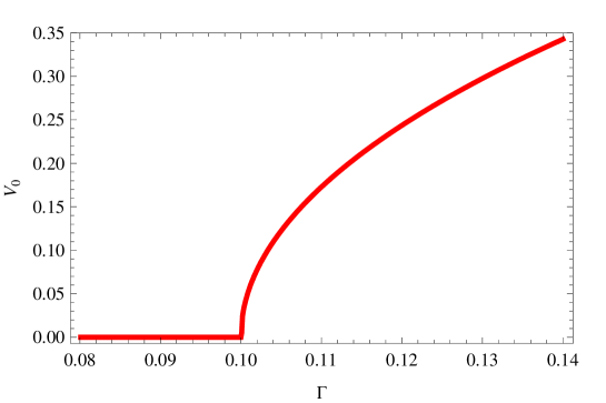
Figure 1: Stable stationary values of $V$. The values of the parameters are $a_{1}=b=D=0.1$, $a_{2}=0.5$, $a_{3}=0$.

which is stable. Note that the transition is continuous at $\Gamma=\Gamma_{c}$. A plot of the bifurcation is given in Fig. 1.

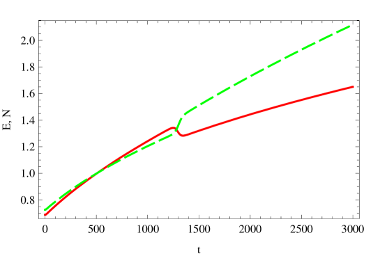
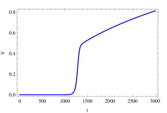
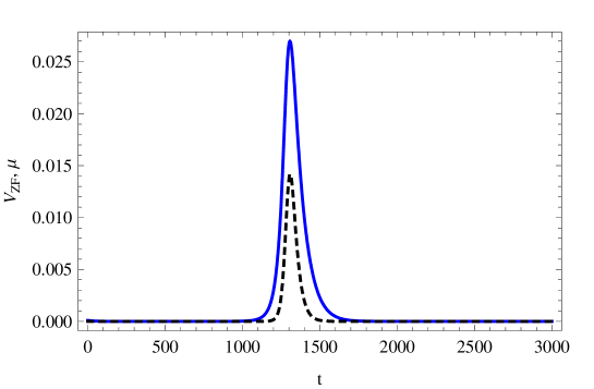
Figure 2: Time-evolution of the variables of the model for $\Gamma(t)=0.05+10^{-4}t$, $a_{1}=b=D=0.1$, $a_{2}=0.5$, and $a_{3}=0$. Top: $E$ (solid) and $N$ (dashed). Middle: $V$. Bottom: $V_{\rm{ZF}}$ (solid) and $\mu$ (dashed). The initial conditions are $V(0)=10^{-3}$, $V_{\rm{ZF}}(0)=10^{-4}$, $E(0)=(\Gamma(0)/D)^{7/13}$, $N(0)=(\Gamma(0)/D)^{6/13}$.

When $a_{3}=0$, the dynamics never reaches an equilibrium solution with $V_{\rm{ZF}}\neq 0$. Equivalently, $V_{\rm{ZF}}$ can be non-zero only transiently. But this is a problem for reproducing the long-range correlations observed during the transition to improved-confinement regimes in TJ-II. The results of Ref. Pedrosa et al. (2008) were obtained in ramping experiments traversing the critical point. In Fig. 2 we show the numerical results from our model when one performs a flux ramp traversing the critical point, going from a low confinement state to an improved confinement one. When $V$ starts growing from zero, and during a short time, $V_{\rm{ZF}}$ follows it and becomes non-zero. However, at a certain moment the inhibition of $V_{\rm{ZF}}$ by $V$ becomes noticeable as $V$ increases and $V_{\rm{ZF}}$ decreases to zero after the transition. The interval of time in which $V_{\rm{ZF}}\neq 0$ coincides with the interval in which $\mu\neq 0$. However, in the experimental data one can see that the correlation has a non-zero stationary value above the critical point.

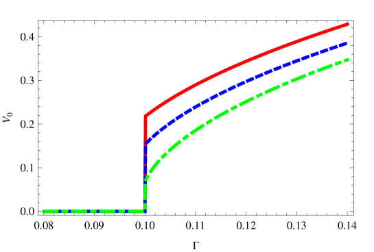
Figure 3: Stable stationary values of $V$. The values of the parameters are $a_{1}=b=D=0.1$, $a_{2}=0.5$, and $a_{3}=0.01$ (solid), $a_{3}=0.005$ (dashed), $a_{3}=0.001$ (long-short dash).

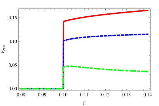
Figure 4: Stable stationary values of $V_{\rm{ZF}}$. The values of the parameters are $a_{1}=b=D=0.1$, $a_{2}=0.5$, and $a_{3}=0.01$ (solid), $a_{3}=0.005$ (dashed), $a_{3}=0.001$ (long-short dash).

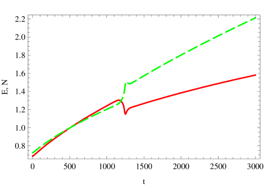
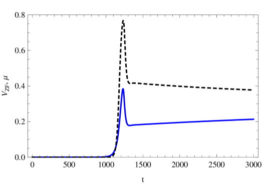
Figure 5: Time-evolution of the variables of the model for the same values of the parameters as in Fig. 2, except that $a_{3}=0.01$.

The situation is very different for $a_{3}>0$. The fixed points (i) and (ii) and their linear stability remain unchanged. However, there is no solution with $V_{\rm{ZF}}=0$ and $V\neq 0$. The third fixed point, corresponding to the high confinement regime and which we will call (iii)^′, has both $V$ and $V_{\rm{ZF}}$ non-zero. In Figs. 3 and 4 we show numerical calculations of the bifurcation for different values of $a_{3}$. The most remarkable feature is that for $a_{3}\neq 0$ the transition is not continuous anymore, but the stationary values of the variables jump at $\Gamma_{c}$. Of course, the magnitude of the jump decreases when $a_{3}$ decreases. Regarding the problem of long-range correlations, it seems essential to have non-zero $a_{3}$. As shown in Fig. 5 this allows to have rampings in which the correlations reach a non-zero stationary value. Although there is no simple analytical expression for the fixed point (iii)^′ for a general value of $\Gamma$, we can give a good approximation for the supercritical solution at $\Gamma=\Gamma_{c}$. Define $\epsilon:=\sqrt{a_{3}}$ and assume

$$E=E_{c}+\epsilon^{2}E_{2}+o(\epsilon^{3}),\quad N=N_{c}+\epsilon^{2}N_{2}+o(\epsilon^{3}),$$ (13a)

$$V=\epsilon V_{1}+o(\epsilon^{2}),\quad V_{\rm{ZF}}=\epsilon V_{\rm{ZF}1}+o(\epsilon^{2}).$$ (13b)

$E_{c}=(b/a_{1})^{7/6}$ and $N_{c}=b/a_{1}$ are the stationary values of $E$ and $N$ for $a_{3}=0$. Introducing this expansion in Eqs. (12) and solving for the lowest order we get:

$$E_{2}=-\frac{3a_{2}}{\sqrt{5}\ a_{1}}\left(\frac{b}{a_{1}}\right)^{5/6}\frac{\sqrt{13\frac{a_{2}}{a_{1}}-20\left(\frac{b}{a_{1}}\right)^{2/3}}}{33a_{2}-20a_{1}\left(\frac{b}{a_{1}}\right)^{2/3}}$$ (14a)

$$N_{2}=-\left(\frac{b}{a_{1}}\right)^{-1/6}E_{2}$$ (14b)

$$V_{1}^{2}=\left(-\frac{13}{6}\left(\frac{b}{a_{1}}\right)^{-1/6}+\frac{10}{3}\frac{a_{1}}{a_{2}}\left(\frac{b}{a_{1}}\right)^{1/2}\right)E_{2}$$ (14c)

$$V_{\rm{ZF}1}^{2}=-\frac{10}{3}\frac{a_{1}}{a_{2}}\left(\frac{b}{a_{1}}\right)^{1/2}E_{2}.$$ (14d)

At this point, we must comment on an issue. In the experiments, that are carried out by means of density ramps, it is difficult to distinguish between a continuous and a discontinuous transition. We can see that by comparing the averaged flows in Figs. 2 and 5. A continuous transition may appear very sharp because the velocity shear grows exponentially in the initial phase. The sharpness depends on the value of this growth rate and on the noise level from where the velocity emerges.

III Comparison of model and experiment

Experiments were carried out in the TJ-II stellarator in Electron Cyclotron Resonance Heated plasmas ($P_{{\rm ECRH}}\leq 400$ kW, $B_{T}=1$ T, $\langle R\rangle=1.5$ m, $\langle a\rangle\leq 0.22$ m, $\lower 3.0pt\hbox{$\mathchar 22\relax$}\mkern-7.0mu\iota(a)\in[1.5,1.9]$). The plasma density was varied in the range $[0.35\cdot 10^{19},1\cdot 10^{19}]{\rm m}^{-3}$. Different edge plasma parameters were simultaneously characterized in two different toroidal positions approximately $160^{\circ}$ apart using two similar multi-Langmuir probes, installed on fast reciprocating drives (approximately $1$ m/s) Pedrosa et al. (1999). For details on the probe arrangement see Ref. Pedrosa et al. (2008). Probe 1 is located in a top window entering vertically through one of the ‘corners’ of its beam-shaped plasma and at $\varphi\approx 35^{\circ}$ (where $\varphi$ is the toroidal angle in the TJ-II reference system). Probe 2 is installed in a bottom window at $\varphi\approx 195^{\circ}$ and enters into the plasma through a region with a higher density of flux surfaces (i.e. lower flux expansion) than Probe 1. It is important to note that the field line passing through one of the probes is approximately $100^{\circ}$ poloidally apart when reaching the toroidal position of the other probe that is more than $5$ m away. Edge radial profiles of different plasma parameters have been measured simultaneously at the two separated toroidal locations with very good agreement. Profiles were obtained in both shot to shot and single shot scenarios with the two probes and in different plasma configurations.

There are five parameters in the model and the $\lambda$ parameter in the determination of the correlation; this is apart from the input function $\Gamma$. The two parameters $b$ and $D$ are directly related to the dissipation terms, viscosity and transport. We determine them from the expected values of those terms at the plasma edge. We take the flow damping rate to be $\nu_{ii}=1.7\cdot 10^{4}\ \rm{s}^{-1}$ and the particle diffusivity $D_{p}=10^{5}\ \rm{cm}^{2}\rm{s}^{-1}$. Therefore, we used $b=D=0.1$. The $a_{1}$ parameter is determined from the criticality condition and the experimental measure of the density profile at the critical point. The measured density profile at about the critical density in TJ-II is such that $N_{c}\approx 1$. Therefore, we take $a_{1}=0.1$.

In this model the long-range correlations are controlled essentially by the ratio $a_{3}/\lambda$. Observe that using Eqs. (13) and (14) we can find an approximate value of the correlation at the critical point:

$$\mu\approx\left(1+\frac{\lambda}{a_{3}}\frac{N_{c}^{-2/3}E_{c}^{2}}{V_{\rm{ZF}1}^{2}}\right)^{-1}.$$ (15)

To have a reasonable level of correlation we need $a_{3}/\lambda$ about 1/3. With the present data it is not possible to distinguish between the two parameters. Therefore, just for convenience,we have taken $a_{3}=0.01$ and $\lambda=0.03$. Finally, the parameter $a_{2}$ has not a very visible impact on the comparison with the data and we have chosen $a_{2}=0.5$.

The input function required in modeling each discharge is the flux function $\Gamma(t)$. Since we are not doing a detailed modeling of data, but only a description of the main features, we have parameterized the flux using only linear dependences in time. A typical example of how the data are described by the model is shown in Figs. 6 and 7, corresponding to discharge 18229. This is a case with a ramp up and down where the plasma crosses the critical point twice, once in the way up and another in the way down. Similar results have been obtained for 10 discharges of TJ-II using the same set of values for the parameters. As one can see in Fig. 6 the parametrization of the flux only gives the main features of the experimental flux. The parameters of this linear function are determined by getting a good description of the density function, which in this case is the ion saturation current. In Fig. 7 we have plotted the ion saturation current, Fig. 7a, the averaged flow velocity shear, Fig. 7b, the ion saturation current fluctuation, Fig. 7c, and the toroidal correlation, Fig. 7d. The agreement between the experimental data and the model description is quite satisfactory, especially noting the extreme simplicity of the latter.

IV Conclusions and further work

Recently, long-distance toroidal correlations in the electrostatic potential fluctuations have been observed in TJ-II Pedrosa et al. (2008). The value of the correlations increases above the critical point of the transition for the emergence of the plasma edge sheared flow layer. In a previous work the transition was interpreted in terms of a simple model Carreras et al. (2006) consisting of envelope equations for the level of fluctuations, the mean flow shear and the averaged pressure gradient.

In the present paper we have shown that the phenomenon of long-distance correlations requires the extension of the model so that the effect of zonal flows is taken into account. With the addition of an equation for the zonal flow amplitude shear the model is able to capture the basic features of the experimental results.

The structure of the model equations is based on quasilinear calculations of resistive pressure-gradient-driven turbulence, and we leave for future publications the detailed calculations which should allow to compute some parameters of the model. Herein, we have determined those parameters by fitting the experimental data.

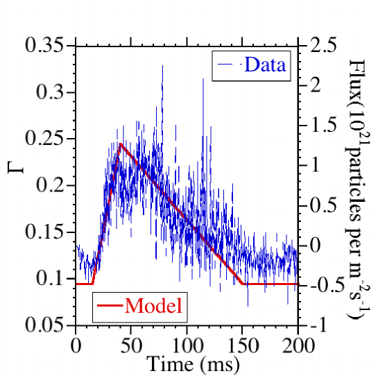
Figure 6: Flux function, $\Gamma(t)$, used in modeling the experimental data.

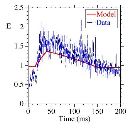
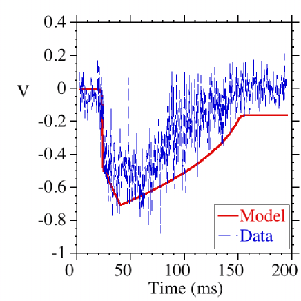
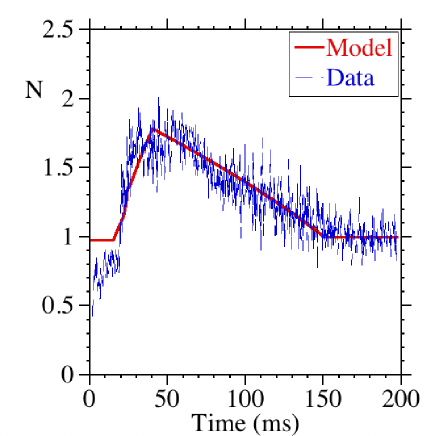
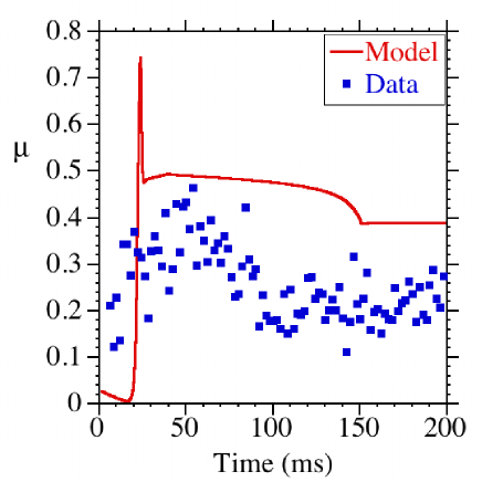
Figure 7: Comparison between the model equations (3) and the experimental data for the shot 18229.