Constraining spins of supermassive black holes from TeV variability. II. fully general relativistic calculations

Abstract

The fast variability of energetic TeV photons from the center of M87 has been detected, offering a new clue to estimate spins of supermassive black holes (SMBHs). We extend the study of Wang et al. (2008) by including all of the general relativistic effects. We numerically solve the full set of relativistic hydrodynamical equations of the radiatively inefficient accretion flows (RIAFs) and then obtain the radiation fields around the black hole. The optical depth of the radiation fields to TeV photons due to pair productions is calculated in the Kerr metric. We find that the optical depth strongly depends on (1) accretion rates as $\tau_{{}_{\rm TeV}}\propto\dot{M}^{2.5-5.0}$; (2) black hole spins; and (3) location of the TeV source. Jointly considering the optical depth and the spectral energy distribution radiated from the RIAFs, the strong degeneration of the spin with the other free parameters in the RIAF model can be largely relaxed. We apply the present model to M87, wherein the RIAFs are expected to be at work, and find that the minimum specific angular momentum of the hole is $a\sim 0.8$. The present methodology is applicable to M87-like sources with future detection of TeV emissions to constrain the spins of SMBHs.

1. Introduction

Astrophysical black holes can be simply depicted by two parameters: mass and angular momentum. Masses of supermassive black holes (SMBHs) are relatively easier to estimate since their gravitational influences spread over the large-scale space approached by Newtonian mechanics. SMBH masses in active galactic nuclei or galactic centers can be measured by several different methods through stellar or gas dynamics, or reverberation mapping of emission lines (Kaspi et al. 2000; Kormendy & Gebhardt 2001; Ho 2008). However, spins are more elusive to estimate because their general relativistic (GR) effects only appear significantly in the innermost region close to the black hole, typically within $\sim$20 gravitational radii and eventually disappear outward then. Spatially resolving the region around $\sim$10 or a few gravitational radii is in principle plausible through radio observations for the Galactic center (Shen et al. 2005; Doeleman et al. 2008), but it is still a limit challenge to current radio astronomy for estimation of the spins of the extragalactic SMBHs.

Hitherto, only a few Seyfert galaxies show relativistically broadened, highly redshifted iron K$\alpha$ emission lines, which are interpreted most plausibly by the collective effects of the Doppler motion of the fluids from which the intrinsic narrow emission lines originate, the gravitational redshift, and the gravitational lensing around a rapidly rotating black hole (see, e.g., Miller 2007 and references therein). The most convincing evidence for effects of spins is found in the MCG-6-30-15 from XMM-Newton observations (Fabian et al. 2002). On the other hand, cosmic X-ray background radiation suggests that most SMBHs are fast rotating (Elvis et al. 2002) and the Soltan’s argument applied to large samples of quasars and galaxies indicates a similar conclusion (Fabian & Iwasawa 1999; Yu & Tremaine 2002; Wang et al. 2006).

TeV photons suffering from attenuation by pair productions are expected to explore the radiation fields in the vicinity of SMBHs and thus constrain their spins (Wang et al. 2008, hereafter Paper I). Rapid variability of TeV emission (at a timescale of 2 days) has been discovered by the HESS (High Energy Stereoscopic System) collaboration in the famous radio galaxy M87 (Aharonian et al. 2006). Interestingly, the TeV emission does not originate from a relativistic jet (Aharonian et al. 2006), in contrast to cases of blazars (Blandford & Levinson 1995; Levinson 2006). A novel mechanism for TeV emission around the horizon of a spinning black hole by a magnetospheric pulsar-like process was originally proposed by Levinson (2000), and had been applied to M87 (Neronov & Aharonian 2007, but see Rieger & Aharonian 2008). In such a context, the TeV photons are able to serve as a probe of spins which determine the density of the radiation fields. Wang et al. (2008) found that the SMBH in M87 should have specific angular momentum $a>0.65$ in order to allow the TeV photons to escape from the innermost region of the radiation fields from the accretion disk. However, their calculations are based on the self-similar solutions of ADAFs in Newtonian approximation and the GR effects on the disk structures and the propagation of photons are not included.

The main goal of this paper is to extend the study of Paper I by including all the GR effects. In Section 2, we introduce the GR RIAF model. Section 3 gives the description of relativistic optics and the detailed formulae used for calculation of optical depth to TeV photons. The results are presented in Section 4 with exhaustive investigation of parameter dependence of the optical depth. We then apply the results to M87 in Section 5. Discussions and a summary are given in Section 6 and 7, respectively. Mathematical preliminaries are presented in the Appendix.

2. General Relativistic RIAF model

We follow the work of Manmoto (2000) to construct the fully relativistic hydrodynamical equations. GR notations are given in the Appendix. Cylindrical coordinates ($t,R,\phi,z$) are used to describe accretion flows by expanding the Boyer$-$Lindquist coordinates around the equatorial plane up to $(z/R)^{0}$ terms. All the basic equations can be derived from the conservation laws of mass, momentum, and energy under the four- dimensional space. For a clarification, we list the necessary equations as follows.

The continuity equation reads

$$\dot{M}=-2\pi\Delta^{1/2}\Sigma_{0}\gamma_{r}V,$$ (1)

where $V$ is the radial velocity of the flows with respect to the corotating reference frame (CRF, see the Appendix) with $\gamma_{r}$ as its Lorentz factor (e.g., Abramowicz et al. 1996; Gammie & Popham 1998; Yuan et al. 2009), $\dot{M}$ is the mass accretion rate, and $\Sigma_{0}$ is the surface density of accretion flows. The conservation of momentum gives two equations. The radial component is

$$\gamma_{r}^{2}V\frac{{\rm d}V}{{\rm d}R}=-\frac{1}{\mu\Sigma_{0}}\frac{{\rm d}W}{{\rm d}R}-\frac{\gamma_{\phi}^{2}AM_{\bullet}}{R^{4}\Delta}\frac{(\Omega-\Omega_{\rm K}^{+})(\Omega-\Omega_{\rm K}^{-})}{\Omega_{\rm K}^{+}\Omega_{\rm K}^{-}},$$ (2)

where $\gamma_{\phi}$ is the Lorentz factor of the azimuthal velocity of the CRF with respect to the locally nonrotating frame (LNRF), the height-integrated total pressure $W$ consists of gas pressure and magnetic pressure, and the relativistic enthalpy $\mu$ is written as

$$\mu=1+\frac{W}{\Sigma_{0}}\left[\left(a_{i}+\frac{1}{\beta_{\rm d}}\right)\frac{W_{i}}{W}+\left(a_{e}+\frac{1}{\beta_{\rm d}}\right)\frac{W_{e}}{W}\right].$$ (3)

Here we express the functions $a_{i}$ and $a_{e}$ as

$$a_{i}=\frac{1}{\gamma_{i}-1}+\frac{2(1-\beta_{\rm d})}{\beta_{\rm d}},$$ (4)

$$a_{e}=\frac{1}{\gamma_{e}-1}+\frac{2(1-\beta_{\rm d})}{\beta_{\rm d}},$$ (5)

with the adiabatic indices of gas $\gamma_{i}$ and $\gamma_{e}$ as

$$\gamma_{i}=1+\theta_{i}\left[\frac{3K_{3}(1/\theta_{i})+K_{1}(1/\theta_{i})}{4K_{2}(1/\theta_{i})}-1\right]^{-1},$$ (6)

$$\gamma_{e}=1+\theta_{e}\left[\frac{3K_{3}(1/\theta_{e})+K_{1}(1/\theta_{e})}{4K_{2}(1/\theta_{e})}-1\right]^{-1},$$ (7)

where the global parameter $\beta_{\rm d}$ is the ratio of the gas pressure to the total pressure, $\theta_{i}=kT_{i}/m_{p}c^{2}$ and $\theta_{e}=kT_{e}/m_{e}c^{2}$ are the dimensionless temperatures of ions ($T_{i}$) and electrons ($T_{e}$), respectively, $k$ is the Boltzmann constant, $m_{p}$ and $m_{e}$ are proton’s and electron’s mass, and $K_{1}$, $K_{2}$, and $K_{3}$ are the modified Bessel functions. The azimuthal component of the conservation of momentum is

$$\dot{M}(\ell-\ell_{\rm in})=2\pi RW_{\phi}^{R},$$ (8)

where $\ell$ is the specific angular momentum of accretion flows, $\ell_{\rm in}$ is the swallowed by the central black hole, and

$$W_{\phi}^{R}=\alpha_{\rm d}\frac{A^{3/2}\Delta^{1/2}\gamma_{\phi}^{3}}{R^{6}}W,$$ (9)

where $\alpha_{\rm d}$ is the viscosity parameter. The conservation of energy for ions and electrons gives

$$-\dot{M}T_{i}\frac{{\rm d}s_{i}}{{\rm d}R}=-2\pi\alpha_{\rm d}(1-\delta)W\frac{\gamma_{\phi}^{4}A^{2}}{R^{6}}\frac{{\rm d}\Omega}{{\rm d}R}-2\pi R\Lambda_{ie},$$ (10)

$$-\dot{M}T_{e}\frac{{\rm d}s_{e}}{{\rm d}R}=-2\pi\alpha_{\rm d}\delta W\frac{\gamma_{\phi}^{4}A^{2}}{R^{6}}\frac{{\rm d}\Omega}{{\rm d}R}+2\pi R(\Lambda_{ie}-F^{-}),$$ (11)

where $s_{i}$ ($s_{e}$) is the specific entropy of ions (electrons), $\Lambda_{ie}$ is the energy transfer rate from the ions to the electrons per unit surface area, and $F^{-}$ is the radiative cooling per unit surface area. $\delta$ is the fraction of the viscous dissipation which heats the electrons. To complete the set of equations, thermal dynamical relations among the entropy, the height-integrated pressure and the surface density for ions and electrons are given by

$$T_{i}{\rm d}s_{i}=\frac{W_{i}}{\Sigma_{i}}\frac{1}{\Gamma_{i}-1}\left[{\rm d}\ln W_{i}-\Gamma_{i}{\rm d}\ln\Sigma_{0}+(\Gamma_{i}-1){\rm d}\ln R\right],$$ (12)

$$T_{e}{\rm d}s_{e}=\frac{W_{e}}{\Sigma_{e}}\frac{1}{\Gamma_{e}-1}\left[{\rm d}\ln W_{e}-\Gamma_{e}{\rm d}\ln\Sigma_{0}+(\Gamma_{e}-1){\rm d}\ln R\right],$$ (13)

where the effective adiabatic indices are

$$\Gamma_{i}=1+\left[a_{i}\left(1+\frac{{\rm d}\ln a_{i}}{{\rm d}\ln T_{i}}\right)\right]^{-1},$$ (14)

$$\Gamma_{e}=1+\left[a_{e}\left(1+\frac{{\rm d}\ln a_{e}}{{\rm d}\ln T_{e}}\right)\right]^{-1}.$$ (15)

The vertical scale height $H$ of the accretion flows is taken as (see also Abramowicz et al. 1997)

$$H^{2}=\frac{\mu W}{\Sigma_{0}}\frac{r^{4}}{\ell^{2}-a^{2}(e^{2}-\mu^{2})},$$ (16)

where $e$ is the specific energy. The simplification ${\rm d}\ln H/{\rm d}\ln R=1$ (Manmoto 2000) is used in deriving the energy equations.

We take into account three processes of the radiative cooling, i.e., the synchrotron radiation, the bremsstrahlung, and the multi-Comptonization of soft photons. The general description of cooling processes and relevant formulae have been presented by Narayan & Yi (1995) and Manmoto (2000) in a more handy way. In our calculations we completely make use of the program of the Comptonization given by Coppi & Blandford (1990).

The outer boundary conditions of the GR RIAF model are imposed at a radius $r_{\rm out}=R_{\rm out}/R_{\rm g}=2\times 10^{4}$:

$$\Omega=0.8\Omega_{\rm K};~{}~{}~{}T_{i}=T_{e}=0.1T_{\rm vir},$$ (17)

where $R_{\rm g}=GM_{\bullet}/c^{2}$ and $T_{\rm vir}$ is the virial temperature defined as

$$T_{\rm vir}=(\gamma-1)\frac{GM_{\bullet}m_{p}}{kR}\approx 1.1(\gamma-1)\times 10^{9}r_{4}^{-1}~{}{\rm K},$$ (18)

with the adiabatic index $\gamma=5/3$ and $r_{4}=r/10^{4}$. Electrons and ions have the same temperature at the outer boundary. As shown by Manmoto et al. (1997), the outer boundary conditions have little influence on the structures of the GR RIAFs. We confirmed this effect and thus fix the outer boundary conditions as Equation (17).

The choice of the eigenvalue $\ell_{\rm in}$ should satisfy the condition that the flows pass through the sonic point smoothly. The inner edge of accretion flows is elusive since it depends on the accretion rate, and is nonaxisymmetric and time-variable (see, e.g., Krolik & Hawley 2002). We use the horizon of the black hole as the inner edge for a conserved influence of the spins on the optical depth of TeV photons. We show this effect of inner edge on uncertainties of spins in the following sections in details.

3. General relativistic optics

3.1. Ray tracing method

We assume that the accretion flows are axisymmetric, so the radiation fields have the same symmetry, and only the motions on the $(R-\theta)$ plane are required in our calculations. The general trajectories of photons in Kerr metric are described by three constants of motion (Bardeen et al. 1972). In terms of the photon’s four-momentum, the conserved quantities are $E=-p_{t}$, the total energy at infinity; $L=p_{\phi}$, the component of angular momentum parallel to symmetry axis and $q=p_{\theta}^{2}+\cos^{2}\theta a^{2}p_{t}^{2}+p_{\phi}^{2}\cot^{2}\theta$. By defining $\lambda=p_{\phi}/E$ and ${\cal Q}=q/E^{2}$, the four-momentum of photons can be rewritten as

$$P_{\mu}=(p_{t},p_{r},p_{\theta},p_{\phi})=\left[-1,\pm\Delta^{-1}\sqrt{{\cal R}(r)},\pm\sqrt{\Theta(\theta)},\lambda\right]E,$$ (19)

where

$${\cal R}(r)=r^{4}+(a^{2}-\lambda^{2}-{\cal Q})r^{2}+2[{\cal Q}+(\lambda-a)^{2}]r-a^{2}{\cal Q},$$ (20)

$$\varTheta(\theta)={\cal Q}+a^{2}\cos^{2}\theta-\lambda^{2}\cot^{2}\theta,$$ (21)

where $r=R/R_{\rm g}$.

Basically, the trajectory of a photon on the ($R-\theta$) plane is governed by the geodesic equations

$${\mathscr{T}}=\pm\int_{r_{0}}^{r}\frac{{\rm d}r}{\sqrt{{\cal R}(r)}}=\pm\int_{\theta_{0}}^{\theta}\frac{{\rm d}\theta}{\sqrt{\Theta(\theta)}}$$ (22)

where ${\mathscr{T}}$ is the affine parameter and the $\pm$ signs represent the increment ($+$) or decrement ($-$) of $r$ and $\theta$ coordinates along the trajectory. The reader is recommended to refer to Rauch & Blandford (1994), Cadez et al. (1998), and Li et al. (2005) for a comprehensive description of the analytic solutions of Equation (22). Given two constants of motion, $\lambda$ and ${\cal Q}$, and the spin parameter $a$, the trajectory of a photon is uniquely determined. We neglect the photons with trajectories returning to the accretion disk but may encounter the TeV photons along their path because of rare probability of occurrence.

3.2. The observed emergent spectrum

The specific flux density observed by a remote observer is expressed as

$$F_{\nu_{\rm o}}=\int I_{\nu_{\rm o}}{\rm d}\Omega_{\rm o},$$ (23)

where $I_{\nu_{\rm o}}$ is the specific intensity as a function of frequency $\nu_{\rm o}$ in the observer’s frame and ${\rm d}\Omega_{\rm o}$ is the element of the solid angle subtended by the image of the accretion disk on the observer’s sky. In a common way, the image of the disk can be described by two impact parameters $\alpha$ and $\beta$ (see Figure 1), which respectively represent the displacement of the image perpendicular to the projection of the rotation of the black hole on the sky and the displacement parallel to the projection of the axis (Li et al. 2005). Applying the invariant $I_{\nu}/\nu^{3}$ along the path of a photon (Rybicki & Lightman 1979, p. 146), we have

$$F_{\nu_{\rm o}}=\int g^{-3}I_{\nu_{\rm e}}\frac{{\rm d}\alpha{\rm d}\beta}{D^{2}},$$ (24)

where $\nu_{\rm e}$ is the frequency of the photons in the local rest frame (LRF) of the accretion flows, $g=\nu_{\rm o}/\nu_{\rm e}$ is the redshift factor of the photons (see Section 3.3), $I_{\nu_{\rm e}}$ is the specific intensity of the disk radiation at radius $r_{\rm e}$, and $D$ is the distance of the black hole from the observer. Then the observed emergent spectrum is

$$L_{\nu_{\rm o}}=4\pi D^{2}F_{\nu_{\rm o}}=4\pi\int g^{-3}I_{\nu_{\rm e}}{\rm d}\alpha{\rm d}\beta.$$ (25)

For each ($\alpha,\beta$) set, the constants of motion $\lambda$ and $\cal Q$ can be expressed as (Li et al. 2005)

$$\lambda=-\alpha\sin\Theta_{\rm obs},~{}~{}~{}~{}{\cal Q}=\beta^{2}+(\alpha^{2}-a^{2})\cos^{2}\Theta_{\rm obs},$$ (26)

where the viewing angle $\Theta_{\rm obs}$ is the inclination between the rotation axis of the accretion disk and the direction to the observer. Using the ray tracing method we can locate the emission place $r_{e}$ in the accretion disk for the photons which reach the observer’s sky at point ($\alpha,\beta$), and, therefore, obtain the radiation intensity $I_{\nu_{\rm e}}$ from the GR RIAF model. The observed emergent spectrum is obtained by integrating $I_{\nu_{\rm e}}$ over the observer’s sky as shown in Equation (25).

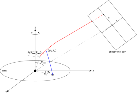
Figure 1.— Geometric scheme. The point $P(R_{\rm TeV},\Theta_{\rm TeV})$ is the location of the TeV source and $Q(r_{\rm c},\theta_{\rm c})$ is the location of the interaction of TeV photons with the soft photons from the RIAFs.

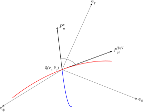
Figure 2.— Locally nonrotating frame at the interacting point $Q(r_{\rm c},\theta_{c})$.

3.3. Optical depth to TeV photons

Figure 1 shows the geometric scheme for calculations of the optical depth to TeV photons which emanate from the position $P(R_{\rm TeV},\Theta_{\rm TeV})$. The TeV photons unavoidably interact with the soft photons from the accretion disk when they are moving out [e.g., at the interacting point $Q(r_{\rm c},\theta_{\rm c})$], setting up strong constraints on the radiation fields of soft photons. We delineate the interactions in the LNRF (see Figure 2). Firstly we divide the solid angle at the interacting point in the LNRF into numerous elements $(\Delta\theta_{\rm s},\Delta\phi_{\rm s})$. For each solid angle element at which the soft photons from the disk arrive, we can determine their constants of motion $\lambda_{\rm s}$ and ${\cal Q}_{\rm s}$ (see Equation (36)). Secondly we use the ray tracing method to trace the soft photons back to the accretion disk. We hence obtain the number density of soft photons. Lastly the optical depth is calculated by integrating all the soft photons from different directions along the trajectory of the TeV photons.

Generally speaking, given the emission location of TeV photons ($R_{\rm TeV}$, $\Theta_{\rm TeV}$) and the viewing angle of an observer ($\Theta_{\rm obs}$), there is a large number of trajectories to the observer at infinity because of the arbitrariness of the $\phi$-component. Since TeV photons along the shortest path intuitively suffer the least interactions and thus undergo the minimum optical depth, we only consider the optical depth for the shortest path in our calculations. We select the trajectory with $\alpha=0$ as the shortest path, which represents the case that the TeV photons lie at the projection of the rotation axis on the image sky. Keep in mind that genuine emission position always has nonzero $\phi$-component, i.e., $\Phi_{\rm TeV}\neq 0$, due to the drag of inertia caused by the rotation of black hole.

In the LNRF, given the frequency of TeV photons $\nu_{\infty}^{\rm TeV}$ at infinity, we can determine their corresponding frequency at the interacting point $Q(r_{\rm c},\theta_{\rm c})$ by redshift factor defined as

$$g_{{}_{\rm TeV}}=\frac{\nu_{\infty}^{\rm TeV}}{\nu_{r_{c}}^{\rm TeV}}=\frac{\left.e^{\mu}_{(t)}P_{\mu}^{\rm TeV}\right|_{\infty}}{\left.e^{\mu}_{(t)}P_{\mu}^{\rm TeV}\right|_{r_{\rm c}}}=\left.\frac{\Sigma^{1/2}\Delta^{1/2}}{A^{1/2}}\frac{1}{1-\omega\lambda_{\rm TeV}}\right|_{r_{\rm c}},$$ (27)

where the subscript $r_{\rm c}$ or $\infty$ means their values are calculated at position ($r_{\rm c},\theta_{\rm c}$) or infinity and similarly hereinafter. In the same way, at the interacting point the frequency of soft photons is given by the redshift factor in comparison with their frequency at the emanating place $r_{\rm d}$ in the accretion disk,

$$g_{\rm s}=\frac{\left.e^{\mu}_{(t)}(\rm LNRF)P_{\mu}^{\rm s}\right|_{r_{\rm c}}}{\left.e^{\mu}_{(t)}(\rm LRF)P_{\mu}^{\rm s}\right|_{r_{\rm d}}}=\frac{\left.e^{-\nu}(1-\omega\lambda_{\rm s})\right|_{r_{c}}}{\left.\gamma_{r}\gamma_{\phi}e^{-\nu}\left[1-\Omega\lambda_{\rm s}\mp\frac{\displaystyle\beta_{r}{\cal R}(r)^{1/2}}{\displaystyle\gamma_{\phi}A^{1/2}}\right]\right|_{r_{\rm d}}}.$$ (28)

The directional angles of the TeV and the soft photons can be obtained from the projection of their four-momentum onto the spatial directions of the LNRF, respectively. The direction cosines ($\alpha_{{}_{\rm TeV}},\beta_{{}_{\rm TeV}},\gamma_{{}_{\rm TeV}}$) of the TeV photons in the LNRF are given by

$$\gamma_{{}_{\rm TeV}}\equiv\cos\theta_{{}_{\rm TeV}}=\frac{\left.e^{\mu}_{(r)}P_{\mu}^{\rm TeV}\right|_{r_{\rm c}}}{-\left.e^{\mu}_{(t)}P_{\mu}^{\rm TeV}\right|_{r_{\rm c}}}=\frac{\pm{\cal R}(r)^{1/2}}{A^{1/2}(1-\omega\lambda_{\rm TeV})},$$ (29)

$$\beta_{{}_{\rm TeV}}\equiv\sin\theta_{{}_{\rm TeV}}\cos\phi_{{}_{\rm TeV}}=\frac{\left.e^{\mu}_{(\theta)}P_{\mu}^{\rm TeV}\right|_{r_{\rm c}}}{-\left.e^{\mu}_{(t)}P_{\mu}^{\rm TeV}\right|_{r_{\rm c}}}=\frac{\pm\Theta(\theta)^{1/2}\Delta^{1/2}}{A^{1/2}(1-\omega\lambda_{\rm TeV})},$$ (30)

$$\alpha_{{}_{\rm TeV}}\equiv\sin\theta_{{}_{\rm TeV}}\sin\phi_{{}_{\rm TeV}}=\frac{\left.e^{\mu}_{(\phi)}P_{\mu}^{\rm TeV}\right|_{r_{\rm c}}}{-\left.e^{\mu}_{(t)}P_{\mu}^{\rm TeV}\right|_{r_{\rm c}}}=\frac{\lambda_{\rm TeV}}{\sin\theta_{\rm c}}\frac{\Sigma\Delta^{1/2}}{A(1-\omega\lambda_{\rm TeV})},$$ (31)

and those of the soft photons are given by replacing the superscript (subscript) “TeV” with “s” in the above equations:

$$\gamma_{\rm s}\equiv\cos\theta_{\rm s}=\frac{\left.e^{\mu}_{(r)}P_{\mu}^{\rm s}\right|_{r_{\rm c}}}{-\left.e^{\mu}_{(t)}P_{\mu}^{\rm s}\right|_{r_{\rm c}}},$$ (32)

$$\beta_{\rm s}\equiv\sin\theta_{\rm s}\cos\phi_{\rm s}=\frac{\left.e^{\mu}_{(\theta)}P_{\mu}^{\rm s}\right|_{r_{\rm c}}}{-\left.e^{\mu}_{(t)}P_{\mu}^{\rm s}\right|_{r_{\rm c}}},$$ (33)

$$\alpha_{\rm s}\equiv\sin\theta_{\rm s}\sin\phi_{\rm s}=\frac{\left.e^{\mu}_{(\phi)}P_{\mu}^{\rm s}\right|_{r_{\rm c}}}{-\left.e^{\mu}_{(t)}P_{\mu}^{\rm s}\right|_{r_{\rm c}}}.$$ (34)

Note that $\alpha_{\rm s}^{2}+\beta_{\rm s}^{2}+\gamma_{\rm s}^{2}=1$, just giving $\alpha_{\rm s}$ and $\beta_{\rm s}$, we can obtain $\lambda_{\rm s}$ and ${\cal Q}_{\rm s}$ from Equations (33) and (34). For simplicity, we define two denotations

$$\mathscr{A}=\frac{\alpha_{\rm s}\sin\theta_{\rm c}A}{\Sigma\Delta^{1/2}},~{}~{}~{}\mathscr{B}=\frac{\beta_{\rm s}A^{1/2}(1-\omega\lambda_{\rm s})}{\Delta^{1/2}},$$ (35)

then we can express $\lambda_{\rm s}$ and ${\cal Q}_{\rm s}$ by $\alpha_{\rm s}$ and $\beta_{\rm s}$ as

$$\lambda_{\rm s}=\frac{\mathscr{A}}{1+\omega\mathscr{A}},~{}~{}~{}{\cal Q}_{\rm s}=\mathscr{B}^{2}-(a\cos\theta_{\rm c})^{2}+(\lambda_{\rm s}\cot\theta_{\rm c})^{2}.$$ (36)

Having obtained $\lambda_{\rm s}$ and ${\cal Q}_{\rm s}$, the ray tracing method is used to determine the emission location $r_{\rm d}$ of the soft photons in the accretion disk.

The number density of the soft photons at the interacting point $(r_{\rm c},\theta_{\rm c})$ is

$$n_{\rm ph}(\theta_{\rm s},\phi_{\rm s},\nu_{\rm s},r_{\rm c},\theta_{\rm c})=\frac{I_{\nu_{\rm s}}}{ch\nu_{\rm s}}=g_{s}^{3}\frac{I_{\nu_{\rm d}}}{ch\nu_{s}},$$ (37)

where $h$ is the Planck’s constant. Here we have applied the invariant $I_{\nu}/\nu^{3}$ along the path of a photon. Finally, the expression for the optical depth of the disk radiation fields to the TeV photons is written as

$$\tau_{{}_{\rm TeV}}(R_{\rm TeV},\Theta_{\rm TeV})=\iiint\sigma_{\gamma\gamma}(\nu_{{}_{\rm TeV}},\nu_{\rm s},\bar{\mu})\frac{I_{\nu_{\rm d}}}{ch\nu_{\rm s}}g_{\rm s}^{3}{\rm d}\Omega{\rm d}\nu_{\rm s}{\rm d}l,$$ (38)

where ${\rm d}l=e^{\nu}\Sigma{\rm d}\mathscr{T}$ is the proper length differential with ${\rm d}\mathscr{T}$ defined to be differential of the affine parameter $\mathscr{T}$ along the TeV photons’ trajectory (see Equation (22)), ${\rm d}\Omega=\sin\theta_{\rm s}d\theta_{\rm s}d\phi_{\rm s}$ is the solid angle element in the LNRF, and $\bar{\mu}$ is the cosine of angle between the TeV photons and the soft photons. The cross-section of the two colliding photons with energy $\epsilon_{{}_{\rm TeV}}=h\nu_{{}_{\rm TeV}}/m_{e}c^{2}$ and $\epsilon_{\rm s}=h\nu_{\rm s}/m_{e}c^{2}$ is given by Gould & Schréder (1967)

$$\sigma_{\gamma\gamma}=\frac{3\sigma_{\rm T}}{16}(1-v^{2})\left[(3-v^{4})\ln\left(\frac{1+v}{1-v}\right)-2v(2-v^{2})\right],$$ (39)

for pair productions, where $\sigma_{\rm T}$ is the Thompson cross-section and $v$ is the velocity of electrons and positrons at the center of momentum frame in units of $c$ related to $\epsilon_{{}_{\rm TeV}}$ and $\epsilon_{\rm s}$ through

$$(1-v^{2})=\frac{2}{(1-\bar{\mu})\epsilon_{s}\epsilon_{{}_{\rm TeV}}}.$$ (40)

The cross section depends on the energies of the interacting photons and their colliding angle. If the two colliding photons run in parallel ($\bar{\mu}=1$), their interaction disappears. The 10TeV photons mostly interact with soft photons of $0.05$eV for header-to-header collisions ($\bar{\mu}=-1$). As shown below, in specific calculations, the energy of soft colliding photons will be modified due to energy shift and bending of their trajectories caused by the GR effects.

It should be pointed out that the GR effects on $\tau_{{}_{\rm TeV}}$ occur through three factors: (1) changing the global structures of RIAFs, as a result, causing dependence of the radiation fields on the spin parameter; (2) modifying the observed spectrum from the RIAFs; and (3) bending the trajectories of TeV photons. For different spins of black holes, the global structures of RIAFs become significantly different starting $\sim$100 $R_{\rm g}$ inward. Once considering the second influence, the observed spectrum is dependent on the viewing angles. The third influence is nonnegligible unless the trajectories of TeV photons closely approach the black hole ($\sim$10 $R_{\rm g}$). These three factors jointly influence the final optical depth to TeV photons.

4. Numerical Results

First, we numerically solve the GR RIAF equations for its structure spanning a large space of parameters. The results are consistent with the numerical solutions in Manmoto (2000). Second, we calculate the intrinsic spectrum for each case of RIAFs with different accretion rates and spins. Third, the ray tracing method is employed to get the spectrum in an observer’s frame. Last, the optical depth to 10TeV photons is calculated along their path from $(R_{\rm TeV},\Theta_{\rm TeV})$ to the observer’s sky at $(\infty,\Theta_{\rm obs})$. The constants of motion $\lambda_{\rm TeV}$ and $\cal Q_{\rm TeV}$ are obtained according to Equation (26), where the impact $\alpha$ is set zero corresponding to the shortest path and $\beta$ is determined by solving the geodesic equations. The properties of structures and emergent spectrum of RIAFs can be found in Manmoto (2000). Here we focus on the optical depth of TeV photons.

Hereinafter we scale accretion rate in the units of the Eddington rate $\dot{M}=\dot{m}\dot{M}_{\rm Edd}$, where $\dot{M}_{\rm Edd}=4\pi GM_{\bullet}m_{p}/\eta\sigma_{\rm T}c$ and $\eta=0.1$ is the radiative efficiency. We set $M_{\bullet}=3.2\times 10^{9}M_{\odot}$ throughout the paper, and $\alpha_{\rm d}=0.1$, $\beta_{\rm d}=0.5$, and $\delta=1.0\times 10^{-3}$ in this section.

4.1. spin dependence

The black hole spins enhance the GR effects on the RIAF structures, the emergent spectrum, and the photon trajectories. Detailed calculations show that both the surface density and the temperature of accretion flows at fixed radius increase with the spins, consequently, making the radiation more efficient with the spins. In light of the drag of the frame, the trajectories of TeV photons will be elongated and the probabilities of pair productions are thus enhanced. These two factors together increase $\tau_{{}_{\rm TeV}}$ with the spins. However, the GR influence on the photon trajectories appears within a radius $\sim$10 $R_{g}$ and, therefore, is less important at relatively large radius.

Figure 3 shows the dependence of $\tau_{{}_{\rm TeV}}$ on the black hole spins for given parameters $\dot{m}=2.5\times 10^{-3}$ and $\Theta_{\rm obs}=\Theta_{\rm TeV}=30^{\circ}$ at four emission radii of TeV photons. Obviously, $\tau_{{}_{\rm TeV}}$ increases with the spins, and its dependence on the spins is more tight at smaller radius because the GR effects become more significant. We can find that $\tau_{{}_{\rm TeV}}\geq 1$ for $a>0.7$ at $R_{\rm TeV}=15R_{\rm g}$. On the other hand, the TeV photons from $R_{\rm TeV}=6R_{\rm g}$ cannot escape from the radiation fields of the GR RIAFs for all spin ranges since $\tau_{{}_{\rm TeV}}\gg 1$.

Figure 3.— Spin dependence of $\tau_{{}_{\rm TeV}}$ for parameters $\dot{m}=2.5\times 10^{-3}$ and $\Theta_{\rm obs}=\Theta_{\rm TeV}=30^{\circ}$ at different $R_{\rm TeV}$.

4.2. $R_{\rm TeV}$ dependence

In Figure 4 we show $\tau_{{}_{\rm TeV}}$ as a strong function of $R_{\rm TeV}$, the radius of the location of TeV photons, by fixing $\dot{m}=2.5\times 10^{-3}$ and $\Theta_{\rm obs}=\Theta_{\rm TeV}=30^{\circ}$. The radiation fields from RIAFs become more and more intensive when $R_{\rm TeV}$ approaches the black hole, leading to a deep dependence of $\tau_{{}_{\rm TeV}}$ on $R_{\rm TeV}$. It is difficult to get an analytical formulation of the dependence, but Figure 4 shows the details of the dependence numerically. The radiation fields from the RIAFs have different spatial distributions with the spins since the GR effects cause their structures distinct. As explained in Section 4.1, the spins enhance the radiation fields. If we fix the energy budget released from the RIAFs, the radiation fields should be more compact for the larger spins, causing a steeper $\tau_{{}_{\rm TeV}}$$-$$R_{\rm TeV}$ relation. The $R_{\rm TeV}$ dependence of $\tau_{{}_{\rm TeV}}$ can be applied to estimate the spins.

4.3. $\Theta_{\rm obs}$ and $\Theta_{\rm TeV}$ dependence

The dependence of $\tau_{{}_{\rm TeV}}$ on $\Theta_{\rm obs}$ and $\Theta_{\rm TeV}$ is caused by the anisotropy of radiation fields from the disk and the dependence of the cross-section on the colliding angle in particular. Generally speaking, the number density of soft photons is mostly contributed from the inner region of the accretion disk. At larger $R_{\rm TeV}$, the path of these photons that reach the interacting point with the TeV photons approximately has the same polar angle with $\Theta_{\rm TeV}$. Since when the two colliding photons run in parallel, their interaction disappears. We can see $\tau_{{}_{\rm TeV}}$ reaches its minimum at $\Theta_{\rm obs}=\Theta_{\rm TeV}$, whereas at smaller $R_{\rm TeV}$, the TeV photons are embedded in the radiation fields from the inner region of the accretion disk and interact with soft photons from all directions and, consequently, it is difficult to give a general explanation to the dependence on $\Theta_{\rm obs}$ and $\Theta_{\rm TeV}$.

We present the $\tau_{{}_{\rm TeV}}$-dependence on $\Theta_{\rm obs}$ and $\Theta_{\rm TeV}$ in Figures 5 and 6, respectively, for the fixed parameters $\dot{m}=6.3\times 10^{-3}$ and $a=0.998$ at different $R_{\rm TeV}$. From Figure 5 we find that (1) for $\Theta_{\rm TeV}=0^{\circ}$, $\tau_{{}_{\rm TeV}}$ monotonously increases with $\Theta_{\rm obs}$, and (2) there is a minimum $\tau_{{}_{\rm TeV}}$ for relatively large $R_{\rm TeV}$ at $\Theta_{\rm obs}=\Theta_{\rm TeV}$. This is confirmed by the case of $\Theta_{\rm TeV}=45^{\circ}$. Figure 6 shows that the $\tau_{{}_{\rm TeV}}$-dependence on $\Theta_{\rm TeV}$ has the similar properties as that on $\Theta_{\rm obs}$.

Figure 4.— $R_{\rm TeV}$ dependence of $\tau_{{}_{\rm TeV}}$ for parameters $a=0.998$, $\dot{m}=2.5\times 10^{-3}$, and $\Theta_{\rm obs}=\Theta_{\rm TeV}=30^{\circ}$.

4.4. $\dot{m}$ dependence

The $\tau_{{}_{\rm TeV}}$-dependence on accretion rates is more straightforward in light of the changes of number density of soft photons and SED from the RIAFs. Figure 7 illustrates how $\tau_{{}_{\rm TeV}}$ changes with accretion rates for fixed parameters $a=0.998$ and $\Theta_{\rm obs}=\Theta_{\rm TeV}=30^{\circ}$. We find that $\tau_{{}_{\rm TeV}}$ is extremely sensitive to accretion rates as $\tau_{{}_{\rm TeV}}\varpropto\dot{m}^{2.5-5.0}$, and the power index tends to be flat at larger $R_{\rm TeV}$. This strongly indicates that TeV photons can be violently diluted by minor changes in accretion rates. In this sense, intensive $\gamma$-ray emission cannot be detected in variable sources. This has important implication in observations.

Figure 5.— $\Theta_{\rm obs}$ dependence of $\tau_{{}_{\rm TeV}}$ for parameters $\dot{m}=6.3\times 10^{-3}$ and $a=0.998$. The solid lines are the results for $\Theta_{\rm TeV}=0^{\circ}$ and the dashed lines are the ones for $\Theta_{\rm TeV}=45^{\circ}$.

Figure 6.— $\Theta_{\rm TeV}$ dependence of $\tau_{{}_{\rm TeV}}$ for parameters $\dot{m}=6.3\times 10^{-3}$ and $a=0.998$. The solid lines are the results for $\Theta_{\rm obs}=0^{\circ}$ and the dashed lines are the ones for $\Theta_{\rm obs}=45^{\circ}$.

This strong dependence can be explained in the following ways. Firstly, RIAFs have properties

$$\Sigma_{0}\sim\dot{m},~{}~{}~{}B\sim\dot{m}^{1/2},~{}~{}~{}\nu_{\rm syn}\sim\gamma_{e}^{2}\dot{m}^{1/2},~{}~{}~{}\tau_{\rm es}\sim\dot{m},$$ (41)

where $B$ is the magnetic field, $\nu_{\rm syn}$ is peak frequency of synchrotron emission, $\gamma_{e}=kT_{e}/m_{e}c^{2}$ is the Lorentz factor of hot thermal electrons, and $\tau_{\rm es}$ is the optical depth for Thompson scattering. The synchrotron emission power approximates as $\sim\gamma_{e}^{2}\Sigma_{0}B^{2}\sim\gamma_{e}^{2}\dot{m}^{2}$ and the bremsstrahlung emission power $\sim\dot{m}^{2}$. In our calculations, we find that $T_{e}\propto\dot{m}^{q}$ and hence $\gamma_{e}\propto\dot{m}^{q}$, where $q\sim 1/3$. To understand the $\tau_{{}_{\rm TeV}}$-dependence on $\dot{m}$, we have to know the energy of soft photons interacting with TeV photons. Figure 8 shows the contribution to $\tau_{{}_{\rm TeV}}$ for soft photons with different frequencies from an RIAF model with $\dot{m}=4.0\times 10^{-3}$, $a=0.998$, $\Theta_{\rm obs}=\Theta_{\rm TeV}=30^{\circ}$, and $R_{\rm TeV}=5R_{\rm g}$. We find that $\nu_{\rm s}\sim 10^{14.5}$Hz, which corresponds to the first Comptonization peak or the second determined by the parameters of the RIAFs. Since RIAFs are optically thin, most of the synchrotron photons escape and a small fraction ($\sim\tau_{\rm es}$) are Compton-scattered by the hot electrons, the energy densities $U_{\rm C_{1}}\propto\gamma_{e}^{2}\dot{m}^{3}\propto\dot{m}^{3+2q}$ and $U_{\rm C_{2}}\propto\gamma_{e}^{2}\dot{m}^{4}\propto\dot{m}^{4+2q}$ for the first and second Comptonization, respectively. This determines the sensitivities of $\tau_{{}_{\rm TeV}}$-dependence on $\dot{m}$ as

$$\tau_{{}_{\rm TeV}}\propto\left\{\begin{array}[]{l}U_{\rm C_{1}}\propto\dot{m}^{3+2q}\sim\dot{m}^{3.7},\\ U_{\rm C_{2}}\propto\dot{m}^{4+2q}\sim\dot{m}^{4.7}.\end{array}\right.$$ (42)

For larger $\dot{m}$, the bremsstrahlung emission will dominate the synchrotron emission and the Comptonization, even at the lower frequency. This leads to a flatter power index $\tau_{{}_{\rm TeV}}\varpropto\dot{m}^{2.5}$. These are nicely consistent with the numerical results as shown in Figure 7.

We would like to point out that the very sensitive dependences of $\tau_{{}_{\rm TeV}}$ on accretion rate as $\tau_{{}_{\rm TeV}}\propto\dot{m}^{2.5-5.0}$ evidently indicate $\tau_{{}_{\rm TeV}}\gg 1$ for the standard accretion disk, immediately drawing a conclusion that the TeV photons cannot escape from the vicinity of SMBH fueled by the standard accretion disk. This is confirmed by the work of Zhang & Cheng (1997).

Figure 7.— $\dot{m}$ dependence of $\tau_{{}_{\rm TeV}}$ for parameters $a=0.998$ and $\Theta_{\rm obs}=\Theta_{\rm TeV}=30^{\circ}$. From the left to the right, the lines correspond to the results for $R_{\rm TeV}=3,4,5,6,10,15,20,30,40R_{\rm g}$, respectively. We can find that $\tau_{{}_{\rm TeV}}\sim\dot{m}^{2.5-5.0}$.

Figure 8.— Contribution to $\tau_{{}_{\rm TeV}}$ from different frequencies of soft photons from the RIAFs with parameters $\dot{m}=4.0\times 10^{-3}$, $a=0.998$, $\Theta_{\rm obs}=\Theta_{\rm TeV}=30^{\circ}$ and $R_{\rm TeV}=5R_{\rm g}$.

5. Application to M87

TeV emission with a rapid variability ($\sim 2$ days) has been detected by the HESS in the giant elliptical galaxy M87, giving clear evidence for a compact TeV emission region in the immediate vicinity of the black hole (Aharonian et al. 2006) and thus providing an opportunity to constrain the spin of the central SMBH. It is well known that M87 hosts an SMBH with $M_{\bullet}=(3.2\pm 0.9)\times 10^{9}M_{\odot}$ (Harms et al. 1994; Macchetto et al. 1997) at a distance of $\sim 16$ Mpc. Table 1 summaries the up-to-date observations from radio to X-ray band as shown in Figure 9 and 10. We exclude the data with low resolution so as to minimize the contamination from the knots in M87. The SED of M87 gives clear evidence for the RIAFs at work in its nucleus (Reynolds et al. 1996; Di Matteo et al. 2003).

Table 1Summary of data for the nucleus of M87.

Frequency	$\nu F_{\nu}$	Resolution	Ref.	Obs.
$\nu$(Hz)	($10^{-13}$erg s-1 cm-2)	(mas)
Radio
$5.0\times 10^{9}$	0.1	0.7	1	VLBI
$2.2\times 10^{10}$	0.48	0.15	2	VLBI
$1.0\times 10^{11}$	8.7	0.1	3	VLBI
IR
$2.8\times 10^{13}$	$46.4\pm 2.5$	460	7	Gemini
Optical-UV
$6.0\times 10^{14}$	$61.7\pm 12.3$	22	6	FOC, HST
$7.0\times 10^{14}$	$20.0$	22	4,5	FOS, HST
$8.1\times 10^{14}$	$37.2\pm 7.4$	22	6	FOC, HST
$9.1\times 10^{14}$	$16.0\pm 1.6$	28.4	9	ACS, HST
$1.2\times 10^{15}$	$14.0\pm 1.4$	28.4	9	ACS, HST
$1.3\times 10^{15}$	$20.4\pm 4.0$	22	6	FOC, HST
$1.9\times 10^{15}$	$12.9\pm 2.5$	22	6	FOC, HST
$2.0\times 10^{15}$	$16.2\pm 3.2$	22	6	FOC, HST
$2.4\times 10^{15}$	$38.9\pm 7.8$	22	6	FOC, HST
X-ray
$2.4\times 10^{17}$	$8.0\pm 0.2$	500	8	Chandra

5.1. Accretion rates of the SMBH

The radiation fields around the black hole can be quantified from the spectral fitting of M87. Before spectral fitting, it is useful to understand to what extent the different parameters influence on the structures of the RIAFs and hence their radiation fields. Small $\alpha_{\rm d}$ indicates the low efficiency of angular momentum transfer, leading to the low radial velocity but high surface density; $\beta_{\rm d}$ represents the fraction of pressure contributed by the gas. As to lower $\beta_{\rm d}$, the structures are changed through two ways: one bt enhancing the magnetic field, and the other by increasing the temperature but reducing the surface density; $\dot{m}$ determines the overall peaks of the spectrum; the parameter $\delta$, representing the fraction of the viscous dissipation that heats electrons, plays an important role in determining the temperature of the electrons and, therefore, in the energy boost of photons after Compton-scattering, i.e., $\delta$ mainly determines the frequency location of the Comptonization bumps. The value of $\delta$ is still open to question at present since some nonthermal mechanisms (e.g., Kolmgorov-like turbulent cascades and collisionless shocks) are highly unclear, which may significantly change the value of $\delta$ (Narayan & Yi 1995). We treat $\delta$ as a free parameter in our calculations. In the spectral fit, we set $\alpha_{\rm d}$ and $\beta_{\rm d}$ a priori to reduce the freedom.

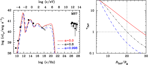
Figure 9.— Left panel: The spectral fit of M87 for Case I (see Table 2). The data from radio to X-ray band are summarized in Table 1 and the TeV data are from the HESS observations (Aharonian et al. 2006). The fit parameters are listed in Table 3. Right panel: The optical depth to 10TeV photons with $\Theta_{\rm TeV}=30^{\circ}$.

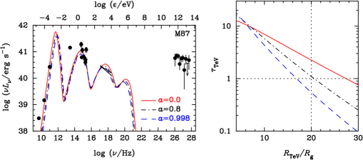
Figure 10.— Same as in Figure 9 but for Case II (see Table 3).

We use the GR RIAF model to fit the multiwavelength spectrum of M87. We firstly fit the observation data used in Paper I (hereafter Case I). We find that $\alpha_{\rm d}=0.025$ and $\beta_{\rm d}=0.2$ give a good fit to the data. $\dot{m}$ and $\delta$ are adjusted with different spins. We furthermore take into account the HST observations (Sparks et al. 1996; Maoz et al. 2005) and redo the fit (hereafter Case II). We set the characteristic value of $\alpha_{\rm d}=0.1$ and $\beta_{\rm d}=0.5$ which means equipartition between the gas and magnetized fields. We present the spectral fit in the left panels of Figures 9 and 10 for Case I and Case II, respectively. The fit parameters are listed in Table 3. The main differences between the two cases are the locations of the multi-Comptonization bumps. In terms of the energy dissipation to heat the electrons, the parameters $\alpha_{\rm d}$ and $\delta$ can be absorbed into one parameter (see Equation (11)). We note that $\delta\alpha_{\rm d}$ of Case II is larger by factor $\sim$4 to that of Case I, which leads to the difference by factor $\sim$4 on the location of the first Comptonization bump.

The accretion rates obtained from fitting of the SED in M87 can be examined independently. Di Matteo et al. (2003) give the Bondi accretion rate of the nucleus of M87 using the Chandra observation as an upper limit of the accretion rate, $\dot{M}<\dot{M}_{\rm Bondi}=1.6\times 10^{-3}\dot{M}_{\rm Edd}$. The accretion rate given by the RIAFs fitting in the current paper is consistent with this upper limit.

We list published literature that gives an estimate of jet power in M87 in Table 2. In regard to the inevitable uncertainties of the estimates, the jet power in M87 is in a range of $10^{42}$$-$$10^{44}$ erg s^-1. There are a number of theoretical calculations of jet power driven by BZ (Blandford$-$Znajek) or BP (Blandford$-$Payne) mechanisms. For example, Meier (2001) developed a hybrid jet model by combining the two processes, in which the jet power is given by

$$\frac{L_{\rm jet}^{\rm Kerr-ADAF}}{L_{\rm acc}}=0.1\left(\alpha_{-1/2}^{\rm ADAF}\right)^{-1}(0.14f^{2}+0.74fj+j^{2})g^{2},$$ (43)

where $f=\Omega_{0}/\Omega_{0,\rm NY}$, $j=cJ/GM^{2}$, $g=B_{\phi,0}/B_{\phi,\rm NY}$, and $L_{\rm acc}=0.1\dot{M}c^{2}$ (see Meier 2001 for details). Taking $f=j=g\sim 1$ and $\alpha=0.1$, the jet power will be $L_{j}\approx 0.6L_{\rm acc}$. Indeed, if considering the field-enhancing shear by frame-dragging effects (Meier 2001, Nemmen et al. 2007), which are neglected in the self-similar solutions, we may have $L_{j}>L_{\rm acc}$, corresponding to extracting the rotational energy from the black hole (the Penrose mechanism). The accretion rates obtained in our paper $\dot{m}\sim 10^{-4}$ are able to produce the jet power $L_{j}>L_{\rm acc}=3\times 10^{43}$ erg s^-1, which generally satisfies the jet energy budget from observations.

Table 2The jet power from the published literature

$L_{j}$/erg s-1	Ref.
$\sim 10^{44}$	Bicknell & Begelman (1996)
$2\times 10^{43}$	Reynolds et al. (1996)
$\sim 10^{44}$	Owen et al. (2000)
$3\times 10^{42}$	Young et al. (2002)
$\sim 10^{44}$	Stawarz et al. (2006)
$5\times 10^{43}$	Bromberg & Levinson (2008)

Table 3The fit parameters ($\Theta_{\rm obs}=30^{\circ}$).

	$a$	$\alpha_{\rm d}$	$\beta_{\rm d}$	$\delta$	$\dot{m}$	$R(\tau_{{}_{\rm TeV}}=1)/R_{\rm g}$
	0.0	0.025	0.20	0.39	$2.0\times 10^{-4}$	28
Case I	0.8	0.025	0.20	0.18	$1.8\times 10^{-4}$	20
	0.998	0.025	0.20	0.09	$1.4\times 10^{-4}$	15
	0.0	0.1	0.5	0.35	$1.0\times 10^{-4}$	28
Case II	0.8	0.1	0.5	0.18	$9.0\times 10^{-5}$	20
	0.998	0.1	0.5	0.11	$7.5\times 10^{-5}$	16

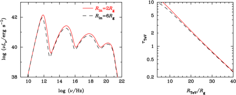
Figure 11.— Influence of the inner edge of the accretion disk on the spectra and $\tau_{{}_{\rm TeV}}$. The parameters are $a=0.0$, $\alpha_{\rm d}=0.1$, $\beta_{\rm d}=0.5$, $\delta=0.35$, $\dot{m}=1.0\times 10^{-4}$, and $\Theta_{\rm TeV}=\Theta_{\rm obs}=30^{\circ}$. For $a=0.998$, the last stable orbit is equal to the gravitational radius.

5.2. Spin of the SMBH

We calculate the optical depth to 10TeV photons and show the results in the right panel of Figures 9 and 10, in which we set $\Theta_{\rm obs}\sim 30^{\circ}$ according to the VLBI observation of the jets in M87 (Bicknell & Begelman 1996) since the jets generally align at the axis of the accretion disk. For both cases, the resultant $\tau_{{}_{\rm TeV}}$$-$$R_{\rm TeV}$ relation becomes steeper with the spins. If we define the transparent radius $R_{c}$ as the radius at which $\tau_{{}_{\rm TeV}}=1$, we find $R_{c}\approx 15R_{\rm g}$ and $28R_{\rm g}$ for $a=0.998$ and $a=0$ in Case I, respectively, and $R_{c}\approx 16R_{\rm g}$ and $28R_{\rm g}$ in Case II. The variability of TeV emission at a timescale of $\sim$2days constrains the emission region $R_{\rm TeV}\leq 20R_{\rm g}$ (Aharonian et al. 2006; Paper I). We find that a black hole with a spin of $a_{{}_{\rm TeV}}=0.8$ for both cases leads to $R_{c}=20R_{\rm g}$. To avoid being optically thick to 10TeV photons, it requires $\tau_{{}_{\rm TeV}}\lesssim 1$ at $R_{\rm TeV}=20R_{\rm g}$. In this sense, the spin of SMBH in M87 should be $a\geq 0.8$ as shown in Figures 9 and 10.

We have to point out that the quality of the current data does not allow us to ascertain which fit is more practical to describe the accretion flows in M87. Future multiwavelength observations with high spatial resolution will provide stronger constraints on the spectrum and hence on the spin of the black hole in M87.

6. Discussions

In this paper we fix the horizon of the black hole as the inner edge of the accretion flows. However, Krolik & Hawley (2002) show that the inner edge of the accretion flows is dependent on the accretion rate and is time-variable. To investigate this effect on the optical depth, we compare the optical depth to 10TeV photons for the cases with inner edges set at the horizon and the last stable orbit, respectively. Figure 11 shows the results with parameters $a=0$ (the horizon is $2R_{\rm g}$ and the last stable orbit is $6R_{\rm g}$), $\alpha_{\rm d}=0.1$, $\beta_{\rm d}=0.5$, $\delta=0.35$, $\dot{m}=1.0\times 10^{-4}$, and $\Theta_{\rm TeV}=\Theta_{\rm obs}=30^{\circ}$. We can clearly see from Figure 11 that the inner edge has little influence on the optical depth of the TeV photons. We presume that the location of TeV origination should be close to the horizon of the black hole. This provides strong constraints on the radiation fields near the black hole horizon. With the detailed calculations presented in this paper, there are still some aspects to be included in the future work.

(1) The size of the TeV source. We simply assume a point-like TeV emission source and neglect its size. Once considering spatial distribution of the source, $\tau_{{}_{\rm TeV}}$ should depend on the location of TeV photons since they have different trajectories. We here only focus on the minimum optical depth; however, the results in the present paper are viable for the current instruments of TeV detection. Future work on the size effects could produce interesting results on variabilities of TeV photons, including the profile of light curves and the time lag between the different TeV photons. This may provide a mapping of the TeV source so that the radiation mechanism will be finally discovered (Böttcher & Dermer 1995; Levinson 2000; Neronov & Aharonian 2007; Rieger & Aharonian 2008).

(2) The motion of the TeV source. For TeV photons with specified trajectory, their optical depth is independent of the properties of the TeV source. However, the beaming effects caused by relativistic motion of the TeV source will help to avoid pair-production absorption of TeV photons, in regard to the beaming of the intensity of TeV photons along the direction of the relativistic motion, and the blueshift of the energy of TeV photons by comparing with that in the source frame. This will modify the observed spectra of TeV emission. Interestingly, the present procedure modified by including beamed TeV photons from relativistic jets can be applied to blazars, which are being powered by the standard accretion disks (in flat spectrum radio quasars) and the RIAFs (in high-frequency peaked BL Lacs, such as Mkn 421 and Mkn 501) (Wang et al. 2003).

(3) The vertical structure of the RIAFs. An exponential profile of the density has been adopted in the vertical direction of the RIAFs, which means that most soft photons are emanating from the midplane. Future three-dimensional simulations of the accretion flows will give a more realistic description of the RIAF structures. In this sense, the optical depth of the TeV photons should be calculated in a more sophisticated way.

(4) The time-dependent trajectories of TeV photons. Future detectors with large area will receive more TeV photons and be able to give more details of spectral variabilities. This needs a consideration on the time-dependent trajectories of TeV photons in light of $\tau_{{}_{\rm TeV}}$ (time-dependent pair productions when $\tau_{{}_{\rm TeV}}>1$), for example, the periodic rotation of the TeV source around the central SMBH. This will definitely provide much more information about the innermost region near the black hole’s horizon.

In other words, further detailed theoretical work is needed for stronger limits on SMBH spins from future observations. The current calculations based on the GR RIAF model provide valuable constraints on the target fields of TeV photons and therefore on the spins.

7. Summary

The optical depth to energetic TeV photons, which are immersed in the radiation fields from radiatively inefficient accretion flows, has been calculated in detail by including all the GR effects. We investigate the dependence of optical depth on the spins ($a$), accretion rates ($\dot{m}$), viewing angles ($\Theta_{\rm obs}$), and location of the TeV photons ($R_{\rm TeV},\Theta_{\rm TeV}$). We find that the optical depth is more sensitive to $R_{\rm TeV}$ than to $\Theta_{\rm obs}$ and $\Theta_{\rm TeV}$. One of the most interesting results is that $\tau_{{}_{\rm TeV}}$ strongly depends on the accretion rates as $\tau_{{}_{\rm TeV}}\propto\dot{m}^{2.5-5.0}$.

Applying the dependence of optical depth on $R_{\rm TeV}$ to constrain the spin parameter in M87, wherein the RIAFs are expected to be at work, we find that the observed TeV photons detected by HESS can escape from the radiation fields from the RIAFs with spin $a\gtrsim 0.8$. Future observations of the phase II HESS with threshold energy one order higher than that of the phase I may discover more M87-like objects (e.g., low-luminosity AGNs) with TeV emission. Hopefully, we then will have a sample for the statistic sample of spins of SMBHs.

Appendix A Preliminaries of GR notations

We adopt geometrical units ($G=c=1$) throughout the Appendix, where $G$ is the gravitational constant and $c$ is the light speed. We use the Kerr metric in Boyer$-$Lindquist coordinates ($t,r,\phi,\theta$)

$${\rm d}s^{2}=-e^{2\nu}{\rm d}t^{2}+e^{2\psi}({\rm d}\phi-\omega{\rm d}t)^{2}+e^{2\mu_{1}}{\rm d}r^{2}+e^{2\mu_{2}}{\rm d}\theta^{2},$$ (A1)

with

$$e^{2\nu}=\frac{\Sigma\Delta}{A},~{}~{}~{}e^{2\psi}=\frac{\sin^{2}\theta A}{\Sigma},$$ (A2)

$$e^{2\mu_{1}}=\frac{\Sigma}{\Delta},~{}~{}~{}e^{2\mu_{2}}=\Sigma,~{}~{}~{}\omega=\frac{2M_{\bullet}ar}{A},$$ (A3)

and

$$\Delta=r^{2}-2M_{\bullet}r+a^{2},~{}~{}~{}\Sigma=r^{2}+a^{2}\cos^{2}\theta,~{}~{}~{}A=(r^{2}+a^{2})^{2}-a^{2}\Delta\sin^{2}\theta,$$ (A4)

where $a=J/M_{\bullet}$ is the specific angular momentum and $M_{\bullet}$ is the black hole mass. The event horizon lies at

$$r_{\rm h}=M_{\bullet}+(M_{\bullet}-a^{2})^{1/2}.$$ (A5)

The angular frequencies of the corotating (+) and counterrotating ($-$) Keplerian motions are

$$\Omega_{\rm K}^{\pm}=\pm\frac{M_{\bullet}^{1/2}}{r^{3/2}\mp aM_{\bullet}^{1/2}}.$$ (A6)

To describe the motions of the accretion flows or photons in Kerr metric, we employ three reference frames (Gammie & Popham 1998). The first is the LNRF, an orthonormal tetrad basis carried by observers who live at constant $r$ and $\theta$, but at $\phi=\omega t~{}+~{}$constant; the second is the CRF, whose coordinate angular velocity is $\Omega$, here $\Omega$ is the angular velocity of the accretion flows. The last is the LRF of the accretion flows. The basis vectors for the LNRF are

$$e^{\mu}_{(t)}=e^{-\nu}(1,0,0,\omega),$$ (A7)

$$e^{\mu}_{(r)}=e^{-\mu_{1}}(0,1,0,0),$$ (A8)

$$e^{\mu}_{(\theta)}=e^{-\mu_{2}}(0,0,1,0),$$ (A9)

$$e^{\mu}_{(\phi)}=e^{-\psi}(0,0,0,1),$$ (A10)

and for the LRF are

$$e^{\mu}_{(t)}=(\gamma_{r}\gamma_{\phi}e^{-\nu},~{}~{}\gamma_{r}\beta_{r}e^{-\mu_{1}},~{}~{}0,~{}~{}\gamma_{r}\gamma_{\phi}e^{-\nu}\Omega),$$ (A11)

$$e^{\mu}_{(r)}=(\gamma_{r}\gamma_{\phi}\beta_{r}e^{-\nu},~{}~{}\gamma_{r}e^{-\mu_{1}},~{}~{}0,~{}~{}\gamma_{r}\gamma_{\phi}\beta_{r}e^{-\nu}\Omega),$$ (A12)

$$e^{\mu}_{(\theta)}=(0,~{}~{}0,~{}~{}e^{-\mu_{2}},~{}~{}0),$$ (A13)

$$e^{\mu}_{(\phi)}=\left[\gamma_{\phi}\beta_{\phi}e^{-\nu},~{}~{}0,~{}~{}0,~{}~{}\gamma_{\phi}(\beta_{\phi}\omega e^{-\nu}+e^{-\psi})\right],$$ (A14)

where $\beta_{r}$ is the radial velocity of the accretion flows in the CRF with $\gamma_{r}=(1-\beta_{r}^{2})^{-1/2}$, $\beta_{\phi}=e^{\psi-\nu}(\Omega-\omega)$ is the physical azimuthal velocity of the CRF with respect to the LNRF with $\gamma_{\phi}=(1-\beta_{\phi}^{2})^{-1/2}$.

References

- Abramowicz et al. (1996) Abramowicz, M. A., Chen, X., Granath, M. & Lasota, J. P. 1996, ApJ, 471, 762
- Abramowicz et al. (1997) Abramowicz, M. A., Lanza, A., Percival, M. J. 1997, ApJ, 479, 179
- Aharonian et al. (2006) Aharonian, A. et al. 2006, Science, 314, 1424
- Bääth et al. (1992) Bääth, B. et al. 1992, A&A, 257, 31
- Bardeen et al. (1972) Bardeen, J. M., Press, W. H. & Teukolsky, S. A. 1972, ApJ, 178, 347