Poisson-Vlasov in a strong magnetic field: A stochastic solution approach

Abstract

Stochastic solutions are obtained for the Maxwell-Vlasov equation in the approximation where magnetic field fluctuations are neglected and the electrostatic potential is used to compute the electric field. This is a reasonable approximation for plasmas in a strong external magnetic field. Both Fourier and configuration space solutions are constructed.

PACS: 52.25Dg, 02.50Ey

Keywords: Poisson-Vlasov, Stochastic solutions

1 Introduction. The notion of stochastic solution

The solutions of linear elliptic and parabolic equations, with Cauchy or Dirichlet boundary conditions, have a probabilistic interpretation. These are classical results which may be traced back to the work of Courant, Friedrichs and Lewy [1] in the 1920’s and became a standard tool in potential theory[2] [3] [4]. A simple example is provided by the heat equation

$$\partial_{t}u(t,x)=\frac{1}{2}\frac{\partial^{2}}{\partial x^{2}}u(t,x)\qquad\mathnormal{with}\qquad u(0,x)=f(x)$$ (1)

with solution written either as

$$u\left(t,x\right)=\frac{1}{\sqrt{2\pi}}\int\frac{1}{\sqrt{t}}\exp\left(-\frac{\left(x-y\right)^{2}}{2t}\right)f\left(y\right)dy$$ (2)

or as

$$u(t,x)=\mathbb{E}_{x}f(X_{t})$$ (3)

$\mathbb{E}_{x}$ denoting the expectation value, starting from $x$, of the process

$$dX_{t}=dW_{t}$$

$W_{t}$ being the Wiener process.

Eq.(1) is a specification of a problem whereas (2) and (3) are solutions in the sense that they both provide algorithmic means to construct a function satisfying the specification. An important condition for (2) and (3) to be considered as solutions is the fact that the algorithms are independent of the particular solution, in the first case an integration procedure and in the second the simulation of a solution-independent process. In both cases the algorithm is the same for all initial conditions. This should be contrasted with stochastic processes constructed from particular solutions, as has been done for example for the Boltzman equation[5].

In contrast with the linear problems, explicit solutions for nonlinear partial differential equations, in terms of elementary functions or integrals, are only known in very particular cases. Hence it is in the field of nonlinear partial differential equations that the stochastic method might be most useful. Whenever a solution-independent stochastic process is found that, for arbitrary initial conditions, generates the solution in the sense of Eq.(3), an exact stochastic solution is obtained. In this way the set of equations for which exact solutions are known might be considerably extended.

The exit measures provided by diffusion plus branching processes[6] [7] [8] [9] [10] [11] as well as the stochastic representations recently constructed for the Navier-Stokes[12] [13] [14] [15] [16] [17], the Poisson-Vlasov[18] [19], the Euler[20] and a nonlinear fractional differential equation[21] define initial condition-independent processes for which the mean values of some functionals are solutions to these equations. Therefore, they are exact stochastic solutions.

Typically, in the stochastic solutions, one deals with a process that starts from the point where the solution is to be found, the solution being then obtained from a functional computed along the whole sample path or until the process hits the boundary. In addition to providing new exact results, the stochastic solutions are also a promising tool for numerical implementation. Here the relevant question is to know when a stochastic algorithm is competitive with the existing deterministic algorithms. Although there is no general answer to this question, there are a few considerations that suggest where and when stochastic algorithms might be useful, namely:

(i) Deterministic algorithms grow exponentially with the dimension $d$ of the space, roughly $N^{d}$ ($\frac{L}{N}$ being the linear size of the grid). This implies that to have reasonable computing times, the number of grid points may not be sufficient to obtain a good local resolution for the solution. In contrast a stochastic simulation only grows with the dimension of the process, typically of order $d$.

(ii) In general, deterministic algorithms aim at obtaining the behavior of the solution in the whole domain. That means that, even if an efficient deterministic algorithm exists for the problem, a stochastic algorithm might still be competitive if only localized values of the solution are desired. This comes from the very nature of the stochastic representation processes that always starts from a definite point in the domain. According to what is desired, configuration or Fourier space representations should be used. For example by studying only a few high Fourier modes one may obtain information on the small scale fluctuations that only a very fine grid would provide in a deterministic algorithm.

(iii) Each time a sample path of the process is implemented, it is independent from any other sample paths that are used to obtain the expectation value. Likewise, paths starting from different points are independent from each other. Therefore the stochastic algorithms are a natural choice for parallel and distributed implementation. Provided some differentiability conditions are satisfied, the process also handles equally well simple or complex boundary conditions.

(iv) Stochastic algorithms may also be used for domain decomposition purposes [22] [23] [24]. One may, for example, decompose the space in subdomains and then use in each one a deterministic algorithm with Dirichlet boundary conditions, the values on the boundaries being determined by a stochastic algorithm.

Stochastic solutions also provide an intuitive characterization of the physical phenomena, relating nonlinear interactions to cascading processes. By the study of exit times from a domain they also provide access to quantities that cannot be obtained by perturbative methods[25] [26].

One way to construct stochastic solutions is based on a probabilistic interpretation of the Picard series. First, the differential equation is written as an integral equation. Then there are two possibilities.

In the first case the series is rearranged in a such a way that the coefficients of the successive terms in the Picard iteration, including the initial condition term, obey a normalization condition. The stochastic solution is then equivalent to importance sampling of the normalized Picard series. In this case the stochastic process, that constructs the solution, is a branching process, the branching being controlled by the nonlinear part of the equation.

The second possibility occurs when the initial condition term is not multiplied by a probability factor. Then, the integral of the integral equation may still be given a probabilistic interpretation but the process that is used for the construction of the solution is more general tree-indexed stochastic process.

In this paper, pursuing the work on kinetic equations initiated in [18] and [19], solutions are obtained for the Maxwell-Vlasov equation in the approximation where magnetic field fluctuations are neglected and the electrostatic potential is used to compute the electric field. This is a reasonable approximation for plasmas in a strong external magnetic field. Both Fourier and configuration space solutions are constructed.

In Sect.2.1 one discusses the formulation of the full Maxwell-Vlasov system as an integral equation for the charge densities. In Sects. 2.1 to 2.4 the solutions to the Fourier-transformed equation are obtained both for a static uniform and a slowly varying magnetic field. The stochastic processes associated to the construction of these solutions are branching processes with the waiting time controlled by the velocity Fourier component and the densities (anti-) evolved by the linear part of the equation.

In Sect.3 one deals with the configuration space equation and in this case the most natural stochastic formulation involves a general tree-indexed stochastic process.

2 The Poisson-Vlasov equation in a magnetic field

2.1 The Maxwell-Vlasov system

Consider a two-species Maxwell-Vlasov system in 3+1 space-time dimensions

$$\frac{\partial f_{i}}{\partial t}+\stackrel{{\scriptstyle\rightarrow}}{{v}}\cdot\nabla_{x}f_{i}+\frac{e_{i}}{m_{i}}\left(\stackrel{{\scriptstyle\rightarrow}}{{E}}+\frac{\stackrel{{\scriptstyle\rightarrow}}{{v}}}{c}\times\stackrel{{\scriptstyle\rightarrow}}{{B}}\right)\cdot\nabla_{v}f_{i}=0$$ (4)

$\left(i=1,2\right)$, with

$$\frac{\partial}{\partial t}\stackrel{{\scriptstyle\rightarrow}}{{E}}-c\nabla_{x}\times\stackrel{{\scriptstyle\rightarrow}}{{B}} = -4\pi\sum_{i}e_{i}\int\stackrel{{\scriptstyle\rightarrow}}{{v}}f_{i}d^{3}v$$

$$\frac{\partial}{\partial t}\stackrel{{\scriptstyle\rightarrow}}{{B}}+c\nabla_{x}\times\stackrel{{\scriptstyle\rightarrow}}{{E}} = 0$$

$$\nabla_{x}\cdot\stackrel{{\scriptstyle\rightarrow}}{{E}} = 4\pi\sum_{i}e_{i}\int f_{i}d^{3}v$$

$$\nabla_{x}\cdot\stackrel{{\scriptstyle\rightarrow}}{{B}} = 0$$ (5)

To study the Vlasov-Maxwell system as a nonlinear equation for the $f_{i}\left(t,x,v\right)$ densities one has to obtain explicit expressions for the electromagnetic fields in terms of the charge densities. Define scalar and vector potentials

$$\stackrel{{\scriptstyle\rightarrow}}{{E}} = -\nabla\phi-\frac{1}{c}\frac{\partial\stackrel{{\scriptstyle\rightarrow}}{{A}}}{\partial t}$$

$$\stackrel{{\scriptstyle\rightarrow}}{{B}} = \nabla\times\stackrel{{\scriptstyle\rightarrow}}{{A}}$$ (6)

which, in the Lorentz gauge ($\nabla\cdot\stackrel{{\scriptstyle\rightarrow}}{{A}}+\frac{1}{c}\frac{\partial\phi}{\partial t}=0$), obey the equations

$$\Delta\phi-\frac{1}{c^{2}}\frac{\partial^{2}\phi}{\partial t^{2}} = -4\pi\sum_{i}e_{i}\int f_{i}d^{3}v$$

$$\Delta\stackrel{{\scriptstyle\rightarrow}}{{A}}-\frac{1}{c^{2}}\frac{\partial^{2}\stackrel{{\scriptstyle\rightarrow}}{{A}}}{\partial t^{2}} = -\frac{4\pi}{c}\sum_{i}e_{i}\int\stackrel{{\scriptstyle\rightarrow}}{{v}}f_{i}d^{3}v$$ (7)

Using the (retarded) Green’s function for the wave equation,

$$G\left(\stackrel{{\scriptstyle\rightarrow}}{{x}}t,\stackrel{{\scriptstyle\rightarrow}}{{x}}^{\prime}t^{{}^{\prime}}\right)=\frac{1}{\left|\stackrel{{\scriptstyle\rightarrow}}{{x}}-\stackrel{{\scriptstyle\rightarrow}}{{x}}^{\prime}\right|}\delta\left(t^{\prime}+\frac{\left|\stackrel{{\scriptstyle\rightarrow}}{{x}}-\stackrel{{\scriptstyle\rightarrow}}{{x}}^{\prime}\right|}{c}-t\right)$$ (8)

one obtains

$$\phi\left(\stackrel{{\scriptstyle\rightarrow}}{{x}},t\right) = \int d^{3}x^{\prime}\frac{1}{\left|\stackrel{{\scriptstyle\rightarrow}}{{x}}-\stackrel{{\scriptstyle\rightarrow}}{{x}}^{\prime}\right|}\sum_{i}e_{i}\int f_{i}\left(\stackrel{{\scriptstyle\rightarrow}}{{x}}^{\prime},\stackrel{{\scriptstyle\rightarrow}}{{v}},t-\frac{\left|\stackrel{{\scriptstyle\rightarrow}}{{x}}-\stackrel{{\scriptstyle\rightarrow}}{{x}}^{\prime}\right|}{c}\right)d^{3}v$$

$$\stackrel{{\scriptstyle\rightarrow}}{{A}}\left(\stackrel{{\scriptstyle\rightarrow}}{{x}},t\right) = \int d^{3}x^{\prime}\frac{1}{\left|\stackrel{{\scriptstyle\rightarrow}}{{x}}-\stackrel{{\scriptstyle\rightarrow}}{{x}}^{\prime}\right|}\sum_{i}\frac{e_{i}}{c}\int\stackrel{{\scriptstyle\rightarrow}}{{v}}f_{i}\left(\stackrel{{\scriptstyle\rightarrow}}{{x}}^{\prime},\stackrel{{\scriptstyle\rightarrow}}{{v}},t-\frac{\left|\stackrel{{\scriptstyle\rightarrow}}{{x}}-\stackrel{{\scriptstyle\rightarrow}}{{x}}^{\prime}\right|}{c}\right)d^{3}v$$ (9)

In writing (9) as a source term solution of (7), one has assumed that the initial conditions for the equations (7) vanish together with their time derivatives or, alternatively, that the initial time is in the remote past so that there are no more contributions from the initial conditions. For a more general solution which should be used for transitory phenomena or plasma probing by short localized pulses see [27].

Use of (6) yields

$$\begin{array}[]{lll}\stackrel{{\scriptstyle\rightarrow}}{{E}}&=&\int d^{3}x^{{}^{\prime}}\sum_{i}e_{i}\frac{1}{\left|x-x^{{}^{\prime}}\right|}\int d^{3}v\left\{\frac{\stackrel{{\scriptstyle\longrightarrow}}{{x-x^{{}^{\prime}}}}}{\left|x-x^{{}^{\prime}}\right|^{2}}+\left(\frac{\stackrel{{\scriptstyle\longrightarrow}}{{x-x^{{}^{\prime}}}}}{c\left|\stackrel{{\scriptstyle\rightarrow}}{{x}}-\stackrel{{\scriptstyle\rightarrow}}{{x}}^{\prime}\right|}-\frac{\stackrel{{\scriptstyle\longrightarrow}}{{v}}}{c^{2}}\right)\partial_{t}\right\}f\left(x^{{}^{\prime}},v,t-\frac{\left|x-x^{{}^{\prime}}\right|}{c}\right)\\ \stackrel{{\scriptstyle\rightarrow}}{{B}}&=&\int d^{3}x^{{}^{\prime}}\sum_{i}\frac{e_{i}}{c}\frac{1}{\left|x-x^{{}^{\prime}}\right|}\int d^{3}vv\times\left\{\frac{\stackrel{{\scriptstyle\longrightarrow}}{{x-x^{{}^{\prime}}}}}{\left|x-x^{{}^{\prime}}\right|^{2}}+\frac{\stackrel{{\scriptstyle\longrightarrow}}{{x-x^{{}^{\prime}}}}}{c\left|\stackrel{{\scriptstyle\rightarrow}}{{x}}-\stackrel{{\scriptstyle\rightarrow}}{{x}}^{\prime}\right|}\partial_{t}\right\}f\left(x^{{}^{\prime}},v,t-\frac{\left|x-x^{{}^{\prime}}\right|}{c}\right)\end{array}$$ (10)

Replacing now Eq.(10) in (4) one sees that, as a function of the densities $f\left(x,v,t\right)$, Maxwell-Vlasov is a nonlinear and nonlocal (in time) differential equation. Its full stochastic solution treatment will be dealt with elsewhere. Here one deals with approximations of practical interest for fusion plasmas. First notice that for non-relativistic plasmas the last terms in (10) are small and in the quasi-static approximation one has

$$\begin{array}[]{lll}\stackrel{{\scriptstyle\rightarrow}}{{E}}&=&\int d^{3}x^{{}^{\prime}}\sum_{i}e_{i}\frac{\stackrel{{\scriptstyle\longrightarrow}}{{x-x^{{}^{\prime}}}}}{\left|x-x^{{}^{\prime}}\right|^{3}}\int d^{3}vf\left(x^{{}^{\prime}},v,t\right)\\ \stackrel{{\scriptstyle\rightarrow}}{{B}}&=&\int d^{3}x^{{}^{\prime}}\sum_{i}\frac{e_{i}}{c}\frac{1}{\left|x-x^{{}^{\prime}}\right|^{3}}\int d^{3}v\left(\stackrel{{\scriptstyle\longrightarrow}}{{v}}\times\left(\stackrel{{\scriptstyle\longrightarrow}}{{x-x^{{}^{\prime}}}}\right)\right)f\left(x^{{}^{\prime}},v,t\right)\end{array}$$ (11)

Furthermore, for microturbulence studies in fusion plasmas in strong magnetic fields, a reasonable approximation neglects magnetic field fluctuations and uses the electrostatic potential of the charges to compute the electric field. This is what will be called Poisson-Vlasov in a static (external) magnetic field.

2.2 Poisson-Vlasov in a static magnetic field

In this approximation the equation is

$$0 = \frac{\partial f_{i}}{\partial t}+\left(\stackrel{{\scriptstyle\rightarrow}}{{v}}\cdot\nabla_{x}+\frac{e_{i}}{m_{i}}\frac{\stackrel{{\scriptstyle\rightarrow}}{{v}}}{c}\times\stackrel{{\scriptstyle\rightarrow}}{{B}}\left(x\right)\cdot\nabla_{v}\right)f_{i}$$ (12)

$$+\frac{e_{i}}{m_{i}}\int d^{3}x^{{}^{\prime}}\sum_{j}e_{j}\int d^{3}uf_{j}\left(x^{{}^{\prime}},u,t\right)\frac{\stackrel{{\scriptstyle\longrightarrow}}{{x-x^{{}^{\prime}}}}}{\left|x-x^{{}^{\prime}}\right|^{3}}\cdot\nabla_{v}f_{i}\left(x,v,t\right)$$

or, in the Fourier transformed version

$$F\left(\xi,t\right)=\frac{1}{\left(2\pi\right)^{3}}\int d^{6}\eta f\left(\eta,t\right)e^{i\xi\cdot\eta}$$ (13)

with $\eta=\left(\stackrel{{\scriptstyle\rightarrow}}{{x}},\stackrel{{\scriptstyle\rightarrow}}{{v}}\right)$ and $\xi=\left(\stackrel{{\scriptstyle\rightarrow}}{{\xi_{1}}},\stackrel{{\scriptstyle\rightarrow}}{{\xi_{2}}}\right)\circeq\left(\xi_{1},\xi_{2}\right)$,

$$\begin{array}[]{ll}\frac{\partial F_{i}\left(\xi,t\right)}{\partial t}&=\left(\stackrel{{\scriptstyle\rightarrow}}{{\xi_{1}}}\cdot\nabla_{\xi_{2}}+\frac{e_{i}}{cm_{i}}\nabla_{\xi_{2}}\times\stackrel{{\scriptstyle\rightarrow}}{{B}}\left(-i\nabla_{\xi_{1}}\right)\cdot\stackrel{{\scriptstyle\rightarrow}}{{\xi_{2}}}\right)F_{i}\left(\xi,t\right)\\ &-\frac{4\pi e_{i}}{m_{i}}\int d^{3}\xi_{1}^{{}^{\prime}}F_{i}\left(\xi_{1}-\xi_{1}^{{}^{\prime}},\xi_{2},t\right)\frac{\stackrel{{\scriptstyle\rightarrow}}{{\xi_{2}}}\cdot\stackrel{{\scriptstyle\rightarrow}}{{\xi_{1}^{{}^{\prime}}}}}{\left|\xi_{1}^{{}^{\prime}}\right|^{2}}\sum_{j}e_{j}F_{j}\left(\xi_{1}^{{}^{\prime}},0,t\right)\end{array}$$ (14)

The aim is to obtain stochastic solutions both for the equation in configuration space and for its Fourier-transformed version. Because of the localized nature of the stochastic solutions, as discussed in the introduction, both types of solutions are useful for the applications. If, in a plasma confinement device, one is interested in the behavior of the solution at a particular point (for example at a point either in the core or in the scrape-off layer) then it is the solution in configuration space that is useful. If however one is interested in the nature of the turbulent fluctuations it is probably the study of high Fourier modes in the Fourier-transformed equation that will be most useful.

Eqs.(12) and (14) have linear and nonlinear parts. The linear evolutions are, respectively

$$\begin{array}[]{lll}f_{i}^{(0)}\left(x,v,t\right)&=&e^{-tQ_{\eta}}f_{i}^{(0)}\left(x,v,0\right)\\ F_{i}^{(0)}\left(\xi_{1},\xi_{2},t\right)&=&e^{-tQ_{\xi}}F_{i}^{(0)}\left(\xi_{1},\xi_{2},0\right)\end{array}$$ (15)

the operators $Q_{\eta}$ and $Q_{\xi}$ being

$$\begin{array}[]{lll}Q_{\eta}&=&\stackrel{{\scriptstyle\rightarrow}}{{v}}\cdot\nabla_{x}+\frac{e_{i}}{cm_{i}}\stackrel{{\scriptstyle\rightarrow}}{{v}}\times\stackrel{{\scriptstyle\rightarrow}}{{B}}\left(x\right)\cdot\nabla_{v}\\ Q_{\xi}&=&-\stackrel{{\scriptstyle\rightarrow}}{{\xi_{1}}}\cdot\nabla_{\xi_{2}}-\frac{e_{i}}{cm_{i}}\nabla_{\xi_{2}}\times\stackrel{{\scriptstyle\rightarrow}}{{B}}\left(-i\nabla_{\xi_{1}}\right)\cdot\stackrel{{\scriptstyle\rightarrow}}{{\xi_{2}}}\end{array}$$ (16)

From (15) and (16) it follows that the linear evolution of the function arguments $x$, $v$, $\xi_{1}$ and $\xi_{2}$ is ruled by the following equations

$$\begin{array}[]{lll}\frac{d}{dt}x\left(t\right)&=&-v\left(t\right)\\ \frac{d}{dt}v\left(t\right)&=&-\frac{e_{i}}{cm_{i}}\left(v\left(t\right)\times B\left(x\left(t\right)\right)\right)\end{array}$$ (17)

$$\begin{array}[]{lll}\frac{d}{dt}\xi_{1}\left(t\right)&=&-\frac{e_{i}}{cm_{i}}\left(\nabla_{\xi_{2}}\left(t\right)\times i\nabla B\left(-i\nabla_{\xi_{1}}\left(t\right)\right)\cdot\xi_{2}\left(t\right)\right)\\ \frac{d}{dt}\xi_{2}\left(t\right)&=&\xi_{1}\left(t\right)+\frac{e_{i}}{cm_{i}}B\left(-i\nabla_{\xi_{1}}\left(t\right)\right)\times\xi_{2}\left(t\right)\end{array}$$ (18)

and

$$\begin{array}[]{lll}\frac{d}{dt}\nabla_{\xi_{1}}\left(t\right)&=&-\nabla_{\xi_{2}}\left(t\right)\\ \frac{d}{dt}\nabla_{\xi_{2}}\left(t\right)&=&-\frac{e_{i}}{cm_{i}}\left(\nabla_{\xi_{2}}\left(t\right)\times B\left(-i\nabla_{\xi_{1}}\left(t\right)\right)\right)\end{array}$$ (19)

One sees from (17) that the linear evolution of the densities $f\left(x,v,t\right)$ in configuration space acts only on the arguments of the function. However, from (18) and (19) one also sees that, if the magnetic field $B$ is not constant in space, the linear evolution of the Fourier transformed densities $F_{i}^{(0)}\left(\xi_{1},\xi_{2},t\right)$ is more complex, involving derivatives of the Fourier density. For the stochastic solutions, one associates a process to each function, therefore it is not convenient to use the full linear part of the evolution operator in the Fourier-transformed equation. Such problem does not exist if the static magnetic field is also uniform in space. Here one starts by studying this case, which is then extended to the case of a slowly varying magnetic field.

2.3 Fourier-transformed Poisson-Vlasov in a static uniform magnetic field

Consider a uniform magnetic field $\stackrel{{\scriptstyle\rightarrow}}{{B}}=\stackrel{{\scriptstyle\rightarrow}}{{B}}_{0}=B_{0}\stackrel{{\scriptstyle\wedge}}{{e_{z}}}$. In this case it is possible to obtain an explicit form for the evolution of the linear part,

$$\left(\begin{array}[]{l}\stackrel{{\scriptstyle\rightarrow}}{{\xi_{1}}}\left(t\right)\\ \stackrel{{\scriptstyle\rightarrow}}{{\xi_{2}}}\left(t\right)\end{array}\right)=e^{t\left(\stackrel{{\scriptstyle\rightarrow}}{{\xi_{1}}}\cdot\nabla_{\xi_{2}}+\frac{e_{i}}{cm_{i}}\nabla_{\xi_{2}}\times\stackrel{{\scriptstyle\rightarrow}}{{B}}_{0}\cdot\stackrel{{\scriptstyle\rightarrow}}{{\xi_{2}}}\right)}\left(\begin{array}[]{l}\stackrel{{\scriptstyle\rightarrow}}{{\xi_{1}}}\\ \stackrel{{\scriptstyle\rightarrow}}{{\xi_{2}}}\end{array}\right)$$ (20)

that is

$$\begin{array}[]{lll}\frac{d}{dt}\stackrel{{\scriptstyle\rightarrow}}{{\xi}}_{1}\left(t\right)&=&0\\ \frac{d}{dt}\stackrel{{\scriptstyle\rightarrow}}{{\xi}}_{2}\left(t\right)&=&\stackrel{{\scriptstyle\rightarrow}}{{\xi_{1}}}\left(t\right)+\frac{e_{i}}{cm_{i}}B_{0}\times\stackrel{{\scriptstyle\rightarrow}}{{\xi_{2}}}\left(t\right)\end{array}$$ (21)

with solution $\stackrel{{\scriptstyle\rightarrow}}{{\xi_{1}}}\left(t\right)=\stackrel{{\scriptstyle\rightarrow}}{{\xi_{1}}}$ and

$$\begin{array}[]{lll}\left(\xi_{2}\left(t\right)\right)_{x}&=&-\left(\xi_{2}\right)_{y}\sin\omega_{i}t+\left(\xi_{2}\right)_{x}\cos\omega_{i}t+\frac{1}{\omega_{i}}\left\{\left(\xi_{1}\right)_{x}\sin\omega_{i}t+\left(\xi_{1}\right)_{y}\left(\cos\omega_{i}t-1\right)\right\}\\ \left(\xi_{2}\left(t\right)\right)_{y}&=&\left(\xi_{2}\right)_{x}\sin\omega_{i}t+\left(\xi_{2}\right)_{y}\cos\omega_{i}t+\frac{1}{\omega_{i}}\left\{\left(\xi_{1}\right)_{x}\left(1-\cos\omega_{i}t\right)+\left(\xi_{1}\right)_{y}\sin\omega_{i}t\right\}\\ \left(\xi_{2}\left(t\right)\right)_{z}&=&\left(\xi_{2}\right)_{z}+t\left(\xi_{1}\right)_{z}\end{array}$$ (22)

with $\omega_{i}=\frac{e_{i}B_{0}}{cm_{i}}$, the inverse relation being

$$\begin{array}[]{ccl}\left(\begin{array}[]{c}\left(\xi_{2}\right)_{x}\\ \left(\xi_{2}\right)_{y}\end{array}\right)&=&\left(\begin{array}[]{ll}\cos\omega_{i}t&\sin\omega_{i}t\\ -\sin\omega_{i}t&\cos\omega_{i}t\end{array}\right)\left(\begin{array}[]{c}\left(\xi_{2}\left(t\right)\right)_{x}-\frac{1}{\omega_{i}}\left(\left(\xi_{1}\right)_{x}\sin\omega_{i}t+\left(\xi_{1}\right)_{y}\left(\cos\omega_{i}t-1\right)\right)\\ \left(\xi_{2}\left(t\right)\right)_{y}-\frac{1}{\omega_{i}}\left\{\left(\xi_{1}\right)_{x}\left(1-\cos\omega_{i}t\right)+\left(\xi_{1}\right)_{y}\sin\omega_{i}t\right\}\end{array}\right)\\ \left(\xi_{2}\right)_{z}&=&\left(\xi_{2}\left(t\right)\right)_{z}-t\left(\xi_{1}\right)_{z}\end{array}$$ (23)

In integral form Eq.(14) becomes

$$F_{i}\left(\xi_{1},\xi_{2},t\right) = F_{i}\left(\xi_{1},\xi_{2}\left(t\right),0\right)-\frac{8\pi e_{i}}{m_{i}}\int_{0}^{t}ds\int d^{3}\xi_{1}^{{}^{\prime}}F_{i}\left(\xi_{1}-\xi_{1}^{{}^{\prime}},\xi_{2}\left(s\right),t-s\right)$$ (24)

$$\times\frac{\stackrel{{\scriptstyle\rightarrow}}{{\xi_{2}}}\left(s\right)\cdot\stackrel{{\scriptstyle\rightarrow}}{{\xi_{1}^{{}^{\prime}}}}}{\left|\xi_{1}^{\prime}\right|^{2}}\sum_{j}\frac{1}{2}e_{j}F_{j}\left(\xi_{1}^{{}^{\prime}},0,t-s\right)$$

A stochastic solution is going to be written for the following function

$$\chi_{i}\left(\xi_{1},\xi_{2},t\right)=e^{-t\gamma\left(\left|\xi_{2}\right|\right)}\frac{F_{i}\left(\xi_{1},\xi_{2},t\right)}{h\left(\xi_{1}\right)}$$ (25)

where $\gamma\left(\left|\xi_{2}\right|\right)=1$ if $\left|\xi_{2}\right|\leq 1$ and $\gamma\left(\left|\xi_{2}\right|\right)=\left|\xi_{2}\right|$ otherwise. $h\left(\xi_{1}\right)$ a positive function to be specified later on. The integral equation for $\chi_{i}\left(\xi_{1},\xi_{2},t\right)$ is

$$\chi_{i}\left(\xi_{1},\xi_{2},t\right) = e^{-t\gamma\left(\left|\xi_{2}\right|\right)}\chi_{i}\left(\xi_{1},\xi_{2}\left(t\right),0\right)-\frac{8\pi e_{i}N\left(\xi_{1},\xi_{2},t\right)}{m_{i}}\frac{\left(\left|\xi_{1}^{\prime}\right|^{-1}h*h\right)\left(\xi_{1}\right)}{h\left(\xi_{1}\right)}$$ (26)

$$\times\int_{0}^{t}ds\frac{\gamma\left(\left|\xi_{2}\left(s\right)\right|\right)}{N\left(\xi_{1},\xi_{2},t\right)}e^{\left(t-s\right)\gamma\left(\left|\xi_{2}\left(s\right)\right|\right)-t\gamma\left(\left|\xi_{2}\right|\right)}\int d^{3}\xi_{1}^{{}^{\prime}}p\left(\xi_{1},\xi_{1}^{{}^{\prime}}\right)\chi_{i}\left(\xi_{1}-\xi_{1}^{{}^{\prime}},\xi_{2}\left(s\right),t-s\right)$$

$$\times\frac{\stackrel{{\scriptstyle\rightarrow}}{{\xi_{2}}}\left(s\right)\cdot\stackrel{{\scriptstyle\wedge}}{{\xi_{1}^{{}^{\prime}}}}}{\gamma\left(\left|\xi_{2}\left(s\right)\right|\right)}\sum_{j}\frac{1}{2}e_{j}\chi_{j}\left(\xi_{1}^{{}^{\prime}},0,t-s\right)$$

with $\stackrel{{\scriptstyle\wedge}}{{\xi_{1}^{{}^{\prime}}}}=\xi_{1}^{{}^{\prime}}/\left|\xi_{1}^{{}^{\prime}}\right|$ ,

$$\left(\left|\xi_{1}^{{}^{\prime}}\right|^{-1}h*h\right)\left(\xi_{1}\right)=\int d^{3}\xi_{1}^{{}^{\prime}}\left|\xi_{1}^{{}^{\prime}}\right|^{-1}h\left(\xi_{1}-\xi_{1}^{{}^{\prime}}\right)h\left(\xi_{1}^{{}^{\prime}}\right)$$ (27)

and

$$p\left(\xi_{1},\xi_{1}^{{}^{\prime}}\right)=\frac{\left|\xi_{1}^{{}^{\prime}}\right|^{-1}h\left(\xi_{1}-\xi_{1}^{{}^{\prime}}\right)h\left(\xi_{1}^{{}^{\prime}}\right)}{\left(\left|\xi_{1}^{{}^{\prime}}\right|^{-1}h*h\right)}$$ (28)

Eq.(26) has a stochastic interpretation as an exponential plus a branching process. The survival probability up to time $t$ of the exponential process is

$$e^{-t\gamma\left(\left|\xi_{2}\right|\right)}$$ (29)

and $ds\Pi\left(\xi_{1},\xi_{2},s\right)$ is the decay probability in time $ds$, with

$$\Pi\left(\xi_{1},\xi_{2},s\right)=\frac{\gamma\left(\left|\xi_{2}\left(s\right)\right|\right)e^{\left(t-s\right)\gamma\left(\left|\xi_{2}\left(s\right)\right|\right)-t\gamma\left(\left|\xi_{2}\right|\right)}}{N\left(\xi_{1},\xi_{2},t\right)}$$ (30)

$N\left(\xi_{1},\xi_{2},t\right)$ being a normalizing function

$$N\left(\xi_{1},\xi_{2},t\right)=\frac{1}{1-e^{-t\gamma\left(\left|\xi_{2}\right|\right)}}\int_{0}^{t}ds\gamma\left(\left|\xi_{2}\left(s\right)\right|\right)e^{\left(t-s\right)\gamma\left(\left|\xi_{2}\left(s\right)\right|\right)-t\gamma\left(\left|\xi_{2}\right|\right)}$$ (31)

In the branching process, $p\left(\xi_{1},\xi_{1}^{{}^{\prime}}\right)d^{3}\xi_{1}^{{}^{\prime}}$ is the probability that, from a $\xi_{1}$ mode, one obtains a $\left(\xi_{1}-\xi_{1}^{{}^{\prime}},\xi_{1}^{{}^{\prime}}\right)$ branching with $\xi_{1}^{{}^{\prime}}$ in the volume $\left(\xi_{1}^{{}^{\prime}},\xi_{1}^{{}^{\prime}}+d^{3}\xi_{1}^{{}^{\prime}}\right)$.

The stochastic interpretation of Eq.(26) provides a way to compute the solution. $\chi_{i}\left(\xi_{1},\xi_{2},t\right)$ is computed from the expectation value of a multiplicative functional associated to the process. Convergence of the multiplicative functional hinges on the fulfilling of the following conditions :

(A) $\left|\frac{F_{i}\left(\xi_{1},\xi_{2},0\right)}{h\left(\xi_{1}\right)}\right|\leq 1$

(B) $\left(\left|\xi_{1}^{{}^{\prime}}\right|^{-1}h*h\right)\left(\xi_{1}\right)\leq h\left(\xi_{1}\right)$

Condition (B) is satisfied, for example, for

$$h\left(\xi_{1}\right)=\frac{c}{\left(1+\left|\xi_{1}\right|^{2}\right)^{2}}\hskip 28.45274pt\mathnormal{and}\hskip 28.45274ptc\leq\frac{1}{3\pi}$$ (32)

Indeed computing $\left|\xi_{1}^{{}^{\prime}}\right|^{-1}h*h$ one obtains

$$\begin{array}[]{lll}c^{2}\Gamma\left(\xi_{1}\right)=\left(\left|\xi_{1}^{{}^{\prime}}\right|^{-1}h*h\right)\left(\xi_{1}\right)&=2\pi c^{2}&\left\{\frac{2\ln\left(1+\left|\xi_{1}\right|^{2}\right)}{\left|\xi_{1}\right|^{2}\left(\left|\xi_{1}\right|^{2}+4\right)^{2}}+\frac{1}{\left|\xi_{1}\right|^{2}\left(\left|\xi_{1}\right|^{2}+4\right)}\right.\\ &&\left.+\frac{\left|\xi_{1}\right|^{2}-4}{2\left|\xi_{1}\right|^{3}\left(\left|\xi_{1}\right|^{2}+4\right)^{2}}\left(\frac{\pi}{2}-\tan^{-1}\left(\frac{2-2\left|\xi_{1}\right|^{2}}{4\left|\xi_{1}\right|}\right)\right)\right\}\end{array}$$ (33)

Then $\frac{1}{h\left(\xi_{1}\right)}\left(\left|\xi_{1}^{{}^{\prime}}\right|^{-1}h*h\right)\left(\xi_{1}\right)$ is bounded by a constant for all $\left|\xi_{1}\right|$, and choosing $c$ sufficiently small, condition (B) is satisfied.

Once $h\left(\xi_{1}\right)$ consistent with (B) is found, condition (A) only puts restrictions on the initial conditions. Now one constructs the following backwards-in-time process, denoted $X\left(\xi_{1},\xi_{2},t\right)$:

Starting at $\left(\xi_{1},\xi_{2},t\right)$, a particle of species $i$ lives for a $\Pi\left(\xi_{1},\xi_{2},s\right)-$distributed time $s$, up to time $t-s$, with survival and decay probabilities given by (29) and (30). At its death a coin $l_{s}$ (probabilities $\frac{1}{2},\frac{1}{2}$) is tossed. If $l_{s}=0$ two new particles of the same species as the original one are born at time $t-s$ with Fourier modes $\left(\xi_{1}-\xi_{1}^{{}^{\prime}},\xi_{2}\left(s\right)\right)$ and $\left(\xi_{1}^{{}^{\prime}},0\right)$ with probability density $p\left(\xi_{1},\xi_{1}^{{}^{\prime}}\right)$. If $l_{s}=1$ the two new particles are of different species. Each one of the newborn particles continues its backward-in-time evolution, following the same decay and branching laws. When one of the particles of this tree reaches time zero it samples the initial condition. The multiplicative functional of the process is the product of the following contributions:

- At each branching point where two particles are born, the coupling constant is

$$g_{ij}\left(\xi_{1},\xi_{1}^{{}^{\prime}},s\right)=-\frac{8\pi e_{i}e_{j}N\left(\xi_{1},\xi_{2},t\right)}{m_{i}}\frac{\left(\left|\xi_{1}^{{}^{\prime}}\right|^{-1}h*h\right)\left(\xi_{1}\right)}{h\left(\xi_{1}\right)}\frac{\stackrel{{\scriptstyle\rightarrow}}{{\xi_{2}}}\left(s\right)\cdot\stackrel{{\scriptstyle\wedge}}{{\xi_{1}^{{}^{\prime}}}}}{\gamma\left(\left|\xi_{2}\left(s\right)\right|\right)}$$ (34)

- When one particle reaches time zero and samples the initial condition the coupling is

$$g_{0i}\left(\xi_{1},\xi_{2}\right)=\frac{F_{i}\left(\xi_{1},\xi_{2},0\right)}{h\left(\xi_{1}\right)}$$ (35)

The multiplicative functional is the product of all these couplings for each realization of the process $X\left(\xi_{1},\xi_{2},t\right)$. The solution $\chi_{i}\left(\xi_{1},\xi_{2},t\right)$ is the expectation value of the multiplicative functional.

$$\chi_{i}\left(\xi_{1},\xi_{2},t\right)=\mathbb{E}\left\{\Pi\left(g_{0}g_{0}^{{}^{\prime}}\cdots\right)\left(g_{ii}g_{ii}^{{}^{\prime}}\cdots\right)\left(g_{ij}g_{ij}^{{}^{\prime}}\cdots\right)\right\}$$ (36)

Fig.1 illustrates a realization of the process. Notice that the label $0\left(s_{3}-s_{1}\right)$ denotes the mode $\xi_{2}=0$ (anti-)evolved during the time $s_{3}-s_{1}$ according to Eq.(22).

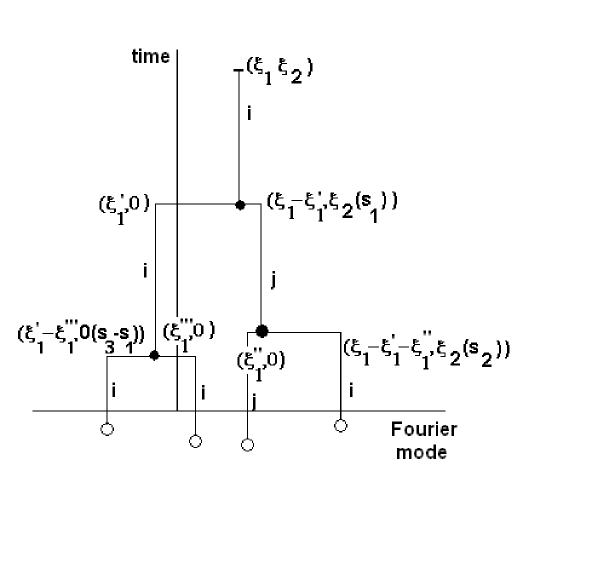
Figure 1: A sample path of the stochastic process $X\left(\xi_{1},\xi_{2},t\right)$

The process itself is the limit of the following iterative process,

$$X_{i}^{\left(k+1\right)}\left(\xi_{1},\xi_{2},t\right)$$

$$= \chi_{i}\left(\xi_{1},\xi_{2}\left(t\right),0\right)\mathbf{1}_{\left[s>\tau\right]}+g_{ii}\left(\xi_{1},\xi_{1}^{{}^{\prime}},s\right)$$

$$\times X_{i}^{\left(k\right)}\left(\xi_{1}-\xi_{1}^{{}^{\prime}},\xi_{2}\left(s\right),t-s\right)X_{i}^{\left(k\right)}\left(\xi_{1}^{{}^{\prime}},0,t-s\right)\mathbf{1}_{\left[s<\tau\right]}\mathbf{1}_{\left[l_{s}=0\right]}$$

$$+g_{ij}\left(\xi_{1},\xi_{1}^{{}^{\prime}},s\right)X_{i}^{\left(k\right)}\left(\xi_{1}-\xi_{1}^{{}^{\prime}},\xi_{2}\left(s\right),t-s\right)X_{j}^{\left(k\right)}\left(\xi_{1}^{{}^{\prime}},0,t-s\right)\mathbf{1}_{\left[s<\tau\right]}\mathbf{1}_{\left[l_{s}=1\right]}$$

with the solution being

$$\chi_{i}\left(\xi_{1},\xi_{2},t\right)=\mathbb{E}\left\{\lim_{k}X_{i}^{\left(k\right)}\left(\xi_{1},\xi_{2},t\right)\right\}$$

With the conditions (A) and (B) and choosing the $c$ constant in $h\left(\xi_{1}\right)$ such that

$$\left|\frac{8\pi e_{i}e_{j}N\left(\xi_{1},\xi_{2},t\right)}{\min_{i}\left\{m_{i}\right\}}\frac{\left(\left|\xi_{1}^{{}^{\prime}}\right|^{-1}h*h\right)}{h\left(\xi_{1}\right)}\right|\leq 1$$ (38)

the absolute value of all coupling constants is bounded by one. The branching process, being identical to a Galton-Watson process, terminates with probability one and the number of inputs to the functional is finite (with probability one). With the bounds on the coupling constants, the multiplicative functional is bounded by one in absolute value almost surely.

Once a stochastic solution is obtained for $\chi_{i}\left(\xi_{1},\xi_{2},t\right)$, one also has, by (24), a stochastic solution for $F_{i}\left(\xi_{1},\xi_{2},t\right)$. Summarizing:

Theorem 1

The stochastic process $X\left(\xi_{1},\xi_{2},t\right)$, above described, provides through the multiplicative functional (36) a stochastic solution of the Fourier-transformed Poisson-Vlasov equation in a uniform magnetic field for arbitrary finite values of the arguments, provided the initial conditions at time zero satisfy the boundedness conditions (A).

2.4 Fourier-transformed Poisson-Vlasov in a static non-uniform magnetic field

The result is now generalized to the case of a static non-uniform magnetic field. Decompose the Fourier transform of the magnetic field into

$$\stackrel{{\scriptstyle\rightarrow}}{{B}}\left(\xi_{1}\right)=\left(2\pi\right)^{3/2}\stackrel{{\scriptstyle\rightarrow}}{{B}}_{0}\delta^{3}\left(\xi_{1}\right)+\stackrel{{\scriptstyle\rightarrow}}{{b}}\left(\xi_{1}\right)$$ (39)

where $\stackrel{{\scriptstyle\rightarrow}}{{B}}_{0}$ might be the average of the field in a region of interest and the non-uniform part $\stackrel{{\scriptstyle\rightarrow}}{{b}}\left(\xi_{1}\right)$ is assumed to be small, in a sense to be specified later. Then the integral equation becomes

$$F_{i}\left(\xi_{1},\xi_{2},t\right) = F_{i}\left(\xi_{1},\xi_{2}\left(t\right),0\right)-\frac{8\pi e_{i}}{m_{i}}\int_{0}^{t}ds\int d^{3}\xi_{1}^{{}^{\prime}}F_{i}\left(\xi_{1}-\xi_{1}^{{}^{\prime}},\xi_{2}\left(s\right),t-s\right)$$ (40)

$$\times\frac{\stackrel{{\scriptstyle\rightarrow}}{{\xi_{2}}}\left(s\right)\cdot\stackrel{{\scriptstyle\rightarrow}}{{\xi_{1}^{{}^{\prime}}}}}{\left|\xi_{1}^{\prime}\right|^{2}}\sum_{j}\frac{1}{2}e_{j}F_{j}\left(\xi_{1}^{{}^{\prime}},0,t-s\right)-\frac{e_{i}}{\left(2\pi\right)^{3/2}cm_{i}}\int_{0}^{t}ds\int d^{3}\xi_{1}^{{}^{\prime}}$$

$$\times\stackrel{{\scriptstyle\rightarrow}}{{\xi_{2}}}\left(s\right)\cdot\left(\stackrel{{\scriptstyle\rightarrow}}{{b}}\left(\xi_{1}^{\prime}\right)\times\bigtriangledown_{\xi_{2}\left(s\right)}\right)F_{i}\left(\xi_{1}-\xi_{1}^{{}^{\prime}},\xi_{2}\left(s\right),t-s\right)$$

where, as before, the dynamics of the arguments $\xi_{2}\left(t\right)$ in $F_{i}$ is controlled by the constant $\stackrel{{\scriptstyle\rightarrow}}{{B}}_{0}$ (Eqs.(21) and (22)). A stochastic solution will be obtained for the function

$$\chi_{i}\left(\xi_{1},\xi_{2},t\right)=e^{-t\gamma\left(\left|\xi_{2}\right|\right)}\frac{F_{i}\left(\xi_{1},\xi_{2},t\right)}{h\left(\xi_{1}\right)}$$ (41)

with integral equation

$$\chi_{i}\left(\xi_{1},\xi_{2},t\right) = e^{-t\gamma\left(\left|\xi_{2}\right|\right)}\chi_{i}\left(\xi_{1},\xi_{2}\left(t\right),0\right)-\frac{e_{i}N\left(\xi_{1},\xi_{2},t\right)}{m_{i}}\frac{\left(\left|\xi_{1}^{\prime}\right|^{-1}h*h\right)\left(\xi_{1}\right)}{h\left(\xi_{1}\right)}\int_{0}^{t}ds\frac{\gamma\left(\left|\xi_{2}\left(s\right)\right|\right)}{N\left(\xi_{1},\xi_{2},t\right)}$$ (42)

$$\times e^{\left(t-s\right)\gamma\left(\left|\xi_{2}\left(s\right)\right|\right)-t\gamma\left(\left|\xi_{2}\right|\right)}\int d^{3}\xi_{1}^{{}^{\prime}}p\left(\xi_{1},\xi_{1}^{{}^{\prime}}\right)\left\{\frac{1}{2}\frac{16\pi\stackrel{{\scriptstyle\rightarrow}}{{\xi_{2}}}\left(s\right)\cdot\stackrel{{\scriptstyle\wedge}}{{\xi_{1}^{{}^{\prime}}}}}{\gamma\left(\left|\xi_{2}\left(s\right)\right|\right)}\sum_{j}\frac{1}{2}e_{j}\chi_{j}\left(\xi_{1}^{{}^{\prime}},0,t-s\right)\right.$$

$$\left.+\frac{1}{2}\frac{2}{\left(2\pi\right)^{3/2}}\frac{\stackrel{{\scriptstyle\rightarrow}}{{\xi_{2}}}\left(s\right)}{\gamma\left(\left|\xi_{2}\left(s\right)\right|\right)}\cdot\left(\frac{\stackrel{{\scriptstyle\rightarrow}}{{b}}\left(\xi_{1}^{{}^{\prime}}\right)}{h\left(\xi_{1}^{{}^{\prime}}\right)}\times\bigtriangledown_{\xi_{2}\left(s\right)}\right)\right\}\chi_{i}\left(\xi_{1}-\xi_{1}^{{}^{\prime}},\xi_{2}\left(s\right),t-s\right)$$

As before, a backwards-in-time process, rooted at $\left(\xi_{1},\xi_{2},t\right)$, is considered. The survival and branching probabilities are also ruled by (29) and (30). However now, whenever the propagating particle dies, there are three distinct possibilities. Either two new particles of the same species (or of opposite species) are born at time $t-s$ with Fourier modes $\left(\xi_{1}-\xi_{1}^{{}^{\prime}},\xi_{2}\left(s\right)\right)$ and $\left(\xi_{1}^{{}^{\prime}},0\right)$ with probability density $p\left(\xi_{1},\xi_{1}^{{}^{\prime}}\right)$ given by (28), or it is just one particle with mode $\left(\xi_{1}-\xi_{1}^{{}^{\prime}},\xi_{2}\left(s\right)\right)$ that is born and the process samples the field $\stackrel{{\scriptstyle\rightarrow}}{{b}}\left(\xi_{1}^{{}^{\prime}}\right)$. That is, the particle samples the non-uniform field and is scattered by it. This particle also receives an operator label

$$K\left(\xi_{1}^{{}^{\prime}},\xi_{2}\left(s\right)\right)=\frac{2}{\left(2\pi\right)^{3/2}}\frac{\stackrel{{\scriptstyle\rightarrow}}{{\xi_{2}}}\left(s\right)}{\gamma\left(\left|\xi_{2}\left(s\right)\right|\right)}\cdot\left(\frac{\stackrel{{\scriptstyle\rightarrow}}{{b}}\left(\xi_{1}^{{}^{\prime}}\right)}{h\left(\xi_{1}^{{}^{\prime}}\right)}\times\bigtriangledown_{\xi_{2}\left(s\right)}\right)$$ (43)

The operator labels are subsequently inherited by the offspring of this particle and accumulate until they are finally applied to those offspring particles that reach time zero. There is no ambiguity in the application of the operators to the final particles because both the $\xi_{2}\left(t\right)$ argument of the final particles and the derivatives $\bigtriangledown_{\xi_{2}\left(s\right)}$ should be expressed in terms of the initial $\xi_{1},\xi_{2},\bigtriangledown_{\xi_{1}},\bigtriangledown_{\xi_{2}}$ using the solutions of Eqs.(18-19).

Denote by $Y\left(\xi_{1},\xi_{2},t\right)$ the process obtained as the iterative limit of the construction described above. A realization of the process is illustrated in Fig.2. The boxed $K\left(\xi_{1}^{{}^{\prime\prime}},\xi_{2}\left(s_{2}\right)\right)$ denotes the operator label that is attached to this particle until it (or its progeny) reaches time zero.

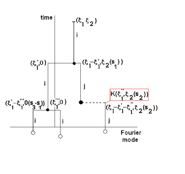
Figure 2: A sample path of the stochastic process $Y\left(\xi_{1},\xi_{2},t\right)$

The solution $\chi_{i}\left(\xi_{1},\xi_{2},t\right)$ of the equation is then obtained from the average value of a multiplicative functional associated to the process. For each realization of the process, the functional is the product of the following factors:

- At each branching point where two particles are born , the coupling constant is

$$g_{ij}\left(\xi_{1},\xi_{1}^{{}^{\prime}},s\right)=-\frac{16\pi e_{i}e_{j}N\left(\xi_{1},\xi_{2},t\right)}{m_{i}}\frac{\left(\left|\xi_{1}^{{}^{\prime}}\right|^{-1}h*h\right)\left(\xi_{1}\right)}{h\left(\xi_{1}\right)}\frac{\stackrel{{\scriptstyle\rightarrow}}{{\xi_{2}}}\left(s\right)\cdot\stackrel{{\scriptstyle\wedge}}{{\xi_{1}^{{}^{\prime}}}}}{\gamma\left(\left|\xi_{2}\left(s\right)\right|\right)}$$ (44)

- When one particle reaches time zero and samples the initial condition the coupling is

$$g_{0i}\left(\xi_{1},\xi_{2}\right)=K\left(\xi_{1}^{{}^{\prime}},\xi_{2}\left(s_{1}\right)\right)K\left(\xi_{1}^{{}^{\prime\prime}},\xi_{2}\left(s_{2}\right)\right)\cdots K\left(\xi_{1}^{{}^{(n)}},\xi_{2}\left(s_{n}\right)\right)\frac{F_{i}\left(\xi_{1},\xi_{2},0\right)}{h\left(\xi_{1}\right)}$$ (45)

In addition to condition (B) of the previous subsection, a sufficient condition for the convergence of the functional is

$$\left|\frac{16\pi e_{i}e_{j}N\left(\xi_{1},\xi_{2},t\right)}{\min_{i}\left\{m_{i}\right\}}\frac{\left(\left|\xi_{1}^{{}^{\prime}}\right|^{-1}h*h\right)}{h\left(\xi_{1}\right)}\right|\leq 1$$ (46)

and

$$\left|K\left(\xi_{1}^{{}^{\prime}},\xi_{2}\left(s_{1}\right)\right)K\left(\xi_{1}^{{}^{\prime\prime}},\xi_{2}\left(s_{2}\right)\right)\cdots K\left(\xi_{1}^{{}^{(n)}},\xi_{2}\left(s_{n}\right)\right)\frac{F_{i}\left(\xi_{1},\xi_{2},0\right)}{h\left(\xi_{1}\right)}\right|\leq 1$$ (47)

for arbitrary $n$ and arbitrary values of the arguments $\xi_{1}^{{}^{\prime}},\xi_{2}\left(s\right)$. This last condition requires boundedness and smoothness of the initial condition as well as a sufficiently small (as compared to $h\left(\xi_{1}\right)$) non-uniformity field $\stackrel{{\scriptstyle\rightarrow}}{{b}}\left(\xi_{1}\right)$. Summarizing:

Theorem 2

The stochastic process $Y\left(\xi_{1},\xi_{2},t\right)$, above described, provides a stochastic solution to the Fourier-transformed Poisson-Vlasov equation in a static non-uniform magnetic field, provided the initial conditions at time zero and the non-uniform part of the field satisfy the condition (47).

2.5 The configuration space equation

Eq.(12) in integral form is

$$f_{i}\left(x,v,t\right) = e^{-tQ_{\eta}}f_{i}\left(x,v,0\right)-\frac{e_{i}}{m_{i}}\int_{0}^{t}dse^{-sQ_{\eta}}\int d^{3}x^{{}^{\prime}}\sum_{j}e_{j}\int d^{3}uf_{j}\left(x^{{}^{\prime}},u,t-s\right)$$ (48)

$$\times\frac{\stackrel{{\scriptstyle\longrightarrow}}{{x-x^{{}^{\prime}}}}}{\left|x-x^{{}^{\prime}}\right|^{3}}\cdot\nabla_{v}f_{i}\left(x,v,t-s\right)$$

or

$$f_{i}\left(x,v,t\right) = f_{i}\left(x\left(t\right),v\left(t\right),0\right)-\frac{e_{i}}{m_{i}}\int_{0}^{t}ds\int d^{3}x^{{}^{\prime}}\sum_{j}e_{j}\int d^{3}uf_{j}\left(x^{{}^{\prime}},u,t-s\right)$$ (49)

$$\times\frac{\stackrel{{\scriptstyle\longrightarrow}}{{x\left(s\right)}}-\stackrel{{\scriptstyle\rightarrow}}{{x^{{}^{\prime}}}}}{\left|x\left(s\right)-x^{{}^{\prime}}\right|^{3}}\cdot\nabla_{v\left(s\right)}f_{i}\left(x\left(s\right),v\left(s\right),t-s\right)$$

$x\left(t\right)$, $v\left(t\right)$ being the solutions of (17) with $x,v$ as initial conditions.

In the Fourier-transformed equation, division by $\gamma\left(\left|\xi_{2}\right|\right)$ not only regularizes the velocity gradient as it also, through multiplication of $F_{i}\left(\xi_{1},\xi_{2},t\right)$ by $e^{-t\gamma\left(\left|\xi_{2}\right|\right)}$, introduces a natural time scale for the exponential process that controls the branching. Here, because division by $\nabla_{v}$ does not make sense, there is no natural exponential time scale. One could nevertheless multiply $f_{i}\left(x,v,t\right)$ by $e^{-\lambda t}$, with $\lambda$ a constant, as in Ref.[20] for the equation without magnetic field. However, because of the nonlinear nature of the second term in (49), this introduces strong limitations on the range of $t$ for which the solution may be constructed. Here a different procedure will be followed. The price to pay is that, instead of a simple branching process, one needs a more complex tree-indexed stochastic process.

Let $G_{i}\left(\stackrel{{\scriptstyle\rightarrow}}{{x}},\stackrel{{\scriptstyle\rightarrow}}{{v}},t\right)$ be the function

$$G_{i}\left(\stackrel{{\scriptstyle\rightarrow}}{{x}},\stackrel{{\scriptstyle\rightarrow}}{{v}},t\right)=\frac{f_{i}\left(\stackrel{{\scriptstyle\rightarrow}}{{x}},\stackrel{{\scriptstyle\rightarrow}}{{v}},t\right)}{\varphi_{i}\left(\stackrel{{\scriptstyle\rightarrow}}{{x}}\left(t\right),\stackrel{{\scriptstyle\rightarrow}}{{v}}\left(t\right)\right)}$$ (50)

the $\varphi\left(\stackrel{{\scriptstyle\rightarrow}}{{x}},\stackrel{{\scriptstyle\rightarrow}}{{v}}\right)$’s being functions to be specified later and $\left(\stackrel{{\scriptstyle\rightarrow}}{{x}}\left(t\right),\stackrel{{\scriptstyle\rightarrow}}{{v}}\left(t\right)\right)$ the function arguments (anti-)evolved by (17). One obtains the following integral equation for $G_{i}\left(\stackrel{{\scriptstyle\rightarrow}}{{x}},\stackrel{{\scriptstyle\rightarrow}}{{v}},t\right)$

$$G_{i}\left(\stackrel{{\scriptstyle\rightarrow}}{{x}},\stackrel{{\scriptstyle\rightarrow}}{{v}},t\right) = G_{i}\left(\stackrel{{\scriptstyle\rightarrow}}{{x}}\left(t\right),\stackrel{{\scriptstyle\rightarrow}}{{v}}\left(t\right),0\right)-2\sum_{j}\frac{1}{2}\frac{e_{i}e_{j}}{m_{i}}\int_{0}^{t}dsA_{x,v,t}^{(j)}$$

$$\times\int d^{3}x^{\prime}d^{3}up_{x,v,t}^{(j)}\left(\stackrel{{\scriptstyle\rightarrow}}{{x^{\prime}}},\stackrel{{\scriptstyle\rightarrow}}{{u}},s\right)G_{j}\left(\stackrel{{\scriptstyle\rightarrow}}{{x^{\prime}}},\stackrel{{\scriptstyle\rightarrow}}{{u}},t-s\right)\widehat{\left(\stackrel{{\scriptstyle\rightarrow}}{{x}}\left(s\right)-\stackrel{{\scriptstyle\rightarrow}}{{x^{\prime}}}\right)}$$

$$\bullet\frac{1}{\varphi_{i}\left(\stackrel{{\scriptstyle\rightarrow}}{{x}}\left(t\right),\stackrel{{\scriptstyle\rightarrow}}{{v}}\left(t\right)\right)}\nabla_{v\left(s\right)}\varphi_{i}\left(\stackrel{{\scriptstyle\rightarrow}}{{x}}\left(t\right),\stackrel{{\scriptstyle\rightarrow}}{{v}}\left(t\right)\right)G_{i}\left(\stackrel{{\scriptstyle\rightarrow}}{{x}}\left(s\right),\stackrel{{\scriptstyle\rightarrow}}{{v}}\left(s\right),t-s\right)$$

with $\widehat{y}=\frac{\stackrel{{\scriptstyle\rightarrow}}{{y}}}{\left|y\right|}$ and

$$p_{x,v,t}^{(j)}\left(\stackrel{{\scriptstyle\rightarrow}}{{x^{\prime}}},\stackrel{{\scriptstyle\rightarrow}}{{u}},s\right)=\frac{1}{A_{x,v,t}^{(j)}}\frac{\varphi_{j}\left(\stackrel{{\scriptstyle\rightarrow}}{{x^{\prime}}}\left(t-s\right),\stackrel{{\scriptstyle\rightarrow}}{{u}}\left(t-s\right)\right)}{\left|\stackrel{{\scriptstyle\rightarrow}}{{x}}\left(s\right)-\stackrel{{\scriptstyle\rightarrow}}{{x^{\prime}}}\right|^{2}}$$ (52)

a probability in the space $[0,t]\times\mathbb{R}^{3}\times\mathbb{R}^{3}$, $A_{x,v,t}$ being the normalization constant

$$A_{x,v,t}^{(j)}=\int_{0}^{t}ds\int\int d^{3}x^{\prime}d^{3}u\frac{\varphi_{j}\left(\stackrel{{\scriptstyle\rightarrow}}{{x^{\prime}}}\left(t-s\right),\stackrel{{\scriptstyle\rightarrow}}{{u}}\left(t-s\right)\right)}{\left|\stackrel{{\scriptstyle\rightarrow}}{{x}}\left(s\right)-\stackrel{{\scriptstyle\rightarrow}}{{x^{\prime}}}\right|^{2}}$$ (53)

One of the simplest choices for the functions $\varphi_{i}\left(\stackrel{{\scriptstyle\rightarrow}}{{x}},\stackrel{{\scriptstyle\rightarrow}}{{v}}\right)$ would be to make it proportional to the initial condition

$$\varphi_{i}\left(\stackrel{{\scriptstyle\rightarrow}}{{x}},\stackrel{{\scriptstyle\rightarrow}}{{v}}\right)=kf_{i}\left(\stackrel{{\scriptstyle\rightarrow}}{{x}},\stackrel{{\scriptstyle\rightarrow}}{{v}},0\right)$$ (54)

Then, the probabilistic interpretation would require finiteness of

$$A_{x,v,t,s}^{(j)}=\int_{0}^{t}ds\int d^{3}x^{\prime}d^{3}u\frac{kf_{j}\left(\stackrel{{\scriptstyle\rightarrow}}{{x^{\prime}}}\left(t-s\right),\stackrel{{\scriptstyle\rightarrow}}{{u}}\left(t-s\right),0\right)}{\left|\stackrel{{\scriptstyle\rightarrow}}{{x}}\left(s\right)-\stackrel{{\scriptstyle\rightarrow}}{{x^{\prime}}}\right|^{2}}$$ (55)

a quantity that has the nature of a retarded field intensity generated by the initial condition. However, the general result will be stated without committing to a particular choice of $\varphi_{i}\left(\stackrel{{\scriptstyle\rightarrow}}{{x}},\stackrel{{\scriptstyle\rightarrow}}{{v}}\right)$.

From Eq.(LABEL:6.4) one sees that because the term $G_{i}\left(\stackrel{{\scriptstyle\rightarrow}}{{x}}\left(t\right),\stackrel{{\scriptstyle\rightarrow}}{{v}}\left(t\right),0\right)$ is not multiplied by a probability factor one cannot simply interpret the construction of $G_{i}\left(\stackrel{{\scriptstyle\rightarrow}}{{x}},\stackrel{{\scriptstyle\rightarrow}}{{v}},t\right)$ as importance sampling of the Picard series. Nevertheless, a probabilistic interpretation may be given through the following tree-indexed stochastic process $Z\left(\stackrel{{\scriptstyle\rightarrow}}{{x}},\stackrel{{\scriptstyle\rightarrow}}{{v}},t\right)$:

Rooted at $\left(\stackrel{{\scriptstyle\rightarrow}}{{x}},\stackrel{{\scriptstyle\rightarrow}}{{u}},t\right)$, a particle of species $i$ propagates backwards-in-time until a time $t-s$ when, controlled by the probability $p_{x,v,t}^{(j)}\left(\stackrel{{\scriptstyle\rightarrow}}{{x^{\prime}}},\stackrel{{\scriptstyle\rightarrow}}{{u}},s\right)$ it gives birth to two new particles. One of them is of the same species $i$ and the other of the same or the opposite species with probability $\frac{1}{2}$. The first particle has coordinates $\left(\stackrel{{\scriptstyle\rightarrow}}{{x}}\left(s\right),\stackrel{{\scriptstyle\rightarrow}}{{v}}\left(s\right)\right)$ and the other coordinates $\left(\stackrel{{\scriptstyle\rightarrow}}{{x^{\prime}}},\stackrel{{\scriptstyle\rightarrow}}{{u}}\right)$ determined by the probability $p_{x,v,t}^{(j)}\left(\stackrel{{\scriptstyle\rightarrow}}{{x^{\prime}}},\stackrel{{\scriptstyle\rightarrow}}{{u}},s\right)$. The first particle also receives an operator label

$$K\left(s\right)=\widehat{\left(\stackrel{{\scriptstyle\rightarrow}}{{x}}\left(s\right)-\stackrel{{\scriptstyle\rightarrow}}{{x^{\prime}}}\right)}\bullet\frac{1}{\varphi_{i}\left(\stackrel{{\scriptstyle\rightarrow}}{{x}}\left(t\right),\stackrel{{\scriptstyle\rightarrow}}{{v}}\left(t\right)\right)}\nabla_{v\left(s\right)}\varphi_{i}\left(\stackrel{{\scriptstyle\rightarrow}}{{x}}\left(t\right),\stackrel{{\scriptstyle\rightarrow}}{{v}}\left(t\right)\right)$$ (56)

to be subsequently applied to all of its offspring. The original particle, the one that gave birth to the two new ones, does not die and proceeds its free propagation until time zero. Then, each one of the newly created particles has an evolution analogous to the progenitor and during the its evolution the operator labels that they inherit at the birth of each new pair are accumulated, until they are finally applied to the initial condition when each one of the particles reaches time zero. A realization of the process is illustrated in Fig.3. The flags, denoted $s_{1},s_{2},\cdots$, stand for the operator labels $K\left(s_{1}\right),K\left(s_{2}\right),\cdots$.

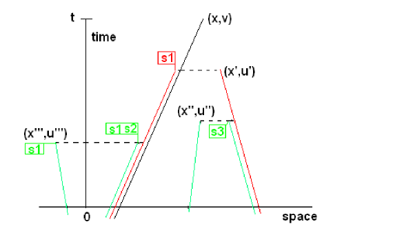
Figure 3: A sample path of the stochastic process $Z\left(\stackrel{{\scriptstyle\rightarrow}}{{x}},\stackrel{{\scriptstyle\rightarrow}}{{v}},t\right)$

The main differences from the Fourier-transformed case are:

- The progenitor particles never die,

- The solution of the equation is obtained from the average over realizations of the following quantities

$$\stackrel{{\scriptstyle\backsim}}{{G}}_{i}\left(\stackrel{{\scriptstyle\rightarrow}}{{x}},\stackrel{{\scriptstyle\rightarrow}}{{v}},t\right) = G_{i}\left(\stackrel{{\scriptstyle\rightarrow}}{{x}}\left(t\right),\stackrel{{\scriptstyle\rightarrow}}{{v}}\left(t\right),0\right)$$

$$-\frac{2e_{i}e_{j}}{m_{i}}A_{x,v,t}^{(j)}\stackrel{{\scriptstyle\backsim}}{{G}}_{j}\left(\stackrel{{\scriptstyle\rightarrow}}{{x^{\prime}}},\stackrel{{\scriptstyle\rightarrow}}{{u}},t-s\right)K\left(s\right)\stackrel{{\scriptstyle\backsim}}{{G}}_{i}\left(\stackrel{{\scriptstyle\rightarrow}}{{x}}\left(s\right),\stackrel{{\scriptstyle\rightarrow}}{{v}}\left(s\right),t-s\right)$$

with $\stackrel{{\scriptstyle\backsim}}{{G}}_{j}\left(\stackrel{{\scriptstyle\rightarrow}}{{x^{\prime}}},\stackrel{{\scriptstyle\rightarrow}}{{u}},t-s\right)$ and $\stackrel{{\scriptstyle\backsim}}{{G}}_{i}\left(\stackrel{{\scriptstyle\rightarrow}}{{x}}\left(s\right),\stackrel{{\scriptstyle\rightarrow}}{{v}}\left(s\right),t-s\right)$ computed in the same way until $t-s$ reaches time zero. For each realization the process runs from time $t$ to zero. However, the calculation of the quantities $\stackrel{{\scriptstyle\backsim}}{{G}}_{i}$ for each realization runs the opposite way, from time zero to time $t$. Qualitatively, what the process does is to replace the calculation of the integrals in (LABEL:6.4) by the generation of a family of probability measures and each value of (2.5) is a sampling of the corresponding Picard iteration.

Assume that, with probability one, the iteration (2.5) converges for all realizations of the process. Then the solution of (LABEL:6.4) is obtained from

$$G_{i}\left(\stackrel{{\scriptstyle\rightarrow}}{{x}},\stackrel{{\scriptstyle\rightarrow}}{{v}},t\right)=\mathbb{E}\left\{\stackrel{{\scriptstyle\backsim}}{{G}}_{i}\left(\stackrel{{\scriptstyle\rightarrow}}{{x}},\stackrel{{\scriptstyle\rightarrow}}{{v}},t\right)\right\}$$ (58)

Hence, existence of the stochastic solution depends on the boundedness and convergence of the iteration in (2.5). Let

$$\left|G_{i}\left(\stackrel{{\scriptstyle\rightarrow}}{{x}},\stackrel{{\scriptstyle\rightarrow}}{{v}},0\right)\right|\leq M$$ (59)

and

$$\left|K\left(s_{1}\right)K\left(s_{2}\right)\cdots K\left(s_{n}\right)G_{i}\left(\stackrel{{\scriptstyle\rightarrow}}{{x}},\stackrel{{\scriptstyle\rightarrow}}{{v}},0\right)\right|\leq M$$ (60)

for all $\stackrel{{\scriptstyle\rightarrow}}{{x}},\stackrel{{\scriptstyle\rightarrow}}{{v}},n$. Then for any arbitrary number of steps in the calculation of (2.5) one would obtain a finite value if

$$8\max\left|\frac{A_{x,v,t}^{(j)}}{m_{i}}\right|M<1$$ (61)

In conclusion:

Theorem 3

If the smoothness and boundedness conditions (59)-(61) are fulfilled, the tree-indexed stochastic process $Z\left(\stackrel{{\scriptstyle\rightarrow}}{{x}},\stackrel{{\scriptstyle\rightarrow}}{{v}},t\right)$ yields a stochastic solution of the configuration space Poisson-Vlasov equation in an external magnetic field.

3 Remarks and conclusions

1) The stochastic solution results established for the Fourier-transformed and the configuration space Poisson-Vlasov equations in an external magnetic field may, as discussed in the introduction, provide adequate algorithms for the parallel computation of localized solutions. That implementation of such algorithms is feasible has been shown in Ref.[19] for the stochastic solutions associated to branching processes and multiplicative functionals. For the Fourier-transformed solutions developed here the algorithms would be quite similar, the main difference being the slightly more complex exponential process. However, this extra complexity pays off in allowing for solutions without upper time bounds.

For the tree-indexed processes, that construct the configuration space solutions, the implementation could lead to larger computer time requirements because, for each realization, one has to compute the iteration in Eq.(2.5) and then to average over many realizations.

2) In plasma phenomena in strong magnetic fields there is a hierarchy of well separated time scales, the Larmor time scale, the bounce time scale and the drift time scale. Separation of the Larmor time scale led to a beautiful body of theory that goes by the name of gyrokinetics[28]. A practical motivation for the gyrokinetics reduction comes from the possibility to reduce the dimension of the numerical codes from 6 to 5 or 4 dimensions. With the present improvement of multiprocessor computer power this motivation has somehow become weaker, especially because of the additional complexity of the gyrokinetics equations if one wants to go beyond the leading order. That, to obtain any reasonable accuracy, higher gyrokinetic orders should be included in the numerical calculation, is indeed to be expected in view of the fact that the exact invariant associated to the gyrokinetics reduction may, at best, be obtained by a Borel-summable infinite series[29]

Nevertheless, if a reduction of the Larmor time scale is desired, the stochastic solution approach developed in this paper might also provide an appropriate framework for this reduction. Notice in particular that, in the configuration space stochastic solutions, the magnetic field evolution acts only on the function arguments, that is, on the labels of the stochastic process not on the process itself. Then, averaging techniques or scalar function mappings would provide an alternative formulation of gyrokinetics.

3) In the stochastic solutions for the configuration space equation and for the non-uniform magnetic field case, operator labels associated to the particles generated in the tree are carried over and applied to the initial conditions when the process arrives to time zero. This entails some additional complexity in the calculation of the functionals and in the smoothness requirements to be imposed on the initial conditions. The need for these operator labels arises from the singular nature of the propagation kernels derivatives. A simple (one-dimensional) example illustrates this point. Let us assume that a probabilistic interpretation is to be given to an integral containing the factor $\partial_{v}f_{i}\left(x,v,t\right)$. Then we may replace it by

$$-\int\delta^{\prime}\left(v-v^{\prime}\right)f_{i}\left(x,v^{\prime},t\right)dv^{\prime}$$

but it is not possible to absorb $\delta^{\prime}\left(v-v^{\prime}\right)$ into a probability kernel unless some limiting approximation is used

$$\int 2\mathnormal{sign}\left(v-v^{\prime}\right)\left|v-v^{\prime}\right|\lim_{\varepsilon\rightarrow 0}\sqrt{\frac{1}{\pi\varepsilon^{3}}}e^{-\frac{\left(v-v^{\prime}\right)^{2}}{\varepsilon}}f_{i}\left(x,v^{\prime},t\right)$$

with sign$\left(v-v^{\prime}\right)$ in the coupling constant and the rest in the probability kernel. However, the computation of the approximation entails numerical instabilities and to keep the derivative as an operator label seems to be a more robust procedure.

A completely different situation occurs if the derivative of the propagation kernel is smooth. This is the case in the Navier-Stokes equation[16], where by an integration by parts the derivative of the heat kernel is controlled by a majorizing kernel and absorbed in the probability measure.

References

[1] R. Courant, K. Friedrichs and H. Lewy; Mat. Ann.
100 (1928) 32-74.
[2] R. M. Blumenthal and R. K. Getoor; Markov
processes and potential theory, Academic Press, New York 1968.
[3] R. F. Bass; Probabilistic techniques in analysis,
Springer, New York 1995.
[4] R. F. Bass; Diffusions and elliptic operators,
Springer, New York 1998.
[5] C. Graham and S. Méléard; in ESAIM Proceedings vol. 10 (F. Coquel and S. Cordier, Eds.) pages 77-126, Les Ulis
2001.
[6] H. P. McKean; Comm. on Pure and Appl. Math. 28
(1975) 323-331, 29 (1976) 553-554.
[7] E. B. Dynkin; Prob. Theory Rel. Fields 89 (1991)
89-115.
[8] E. Dynkin; Ann. Probab. 19 (1991) 1157-1194.
[9] E. B. Dykin; Ann. Probab. 21 (1993) 1185-1262.
[10] E. B. Dynkin; Diffusions, Superdiffusions and
Partial Differential Equations, AMS Colloquium Pubs., Providence
2002.
[11] E. Dynkin; Superdiffusions and positive solutions
of nonlinear partial differential equations, AMS , Providence.
[12] Y. LeJan and A. S. Sznitman ; Prob. Theory and Relat.
Fields 109 (1997) 343-366.
[13] E. C. Waymire; Prob. Surveys 2 (2005) 1-32.
[14] E. Waymire; Lectures on multiscale and
multiplicative processes, www.maphysto.dk/publications/MPS-LN/2002/11.pdf
[15] R. N. Bhattacharya et al. ; Trans. Amer. Math.
Soc. 355 (2003) 5003-5040
[16] M. Ossiander ; Prob. Theory and Relat. Fields
133 (2005) 267-298.
[17] J. C. Orum; Stochastic cascades and 2D Fourier
Navier-Stokes equations, in Lectures on multiscale and
multiplicative processes, www.maphysto.dk/publications/MPS-LN/2002/11.pdf
[18] R. Vilela Mendes and F. Cipriano; Comm. Nonlin.
Sci. and Num. Simul. 13 (2008) 221-226 and 1736.
[19] E. Floriani, R. Lima and R. Vilela Mendes; European Physical Journal D 46 (2008) 295-302 and 407.
[20] R. Vilela Mendes; Stochastic solutions of some
nonlinear partial differential equations, Stochastics 81 (2009)
279-297.
[21] F. Cipriano, H. Ouerdiane and R. Vilela Mendes; Fract. Calc. Appl. Anal. 12 (2009) 47-56.
[22] J. A. Acebrón, M. P. Busico, P. Lanucara and R.
Spigler; SIAM J. Sci. Comput. 27 (2005) 440-457.
[23] J. A. Acebrón and R. Spigler; Lect. Notes in
Comput. Sci. and Eng. 55 (2007) 475-480.
[24] D. Talay and L. Tubaro; Probabilistic models for
nonlinear partial differential equations, Lecture Notes in
Mathematics 1627, 1996.
[25] S. M. Eleutério and R. Vilela Mendes; J.
Phys. A 20 (1987) 6411.
[26] R. Vilela Mendes; Zeitsch. Phys. C 54, (1992)
273-281.
[27] N. Roy; Lorentz gauge and Green’s formula in
classical electrodynamics, arXiv:hep-th/9607205.
[28] A. J. Brizard and T. S. Hahm; Rev. Mod. Phys. 79
(2007) 421-468.
[29] P. Ghendrih, R. Lima and R. Vilela Mendes; J.
Phys. A: Math. Theor.41 (2008) 465501.