A projection proximal-point algorithm for $\ell^{1}$-minimization

Abstract

The problem of the minimization of least squares functionals with $\ell^{1}$ penalties is considered in an infinite dimensional Hilbert space setting. While there are several algorithms available in the finite dimensional setting there are only a few of them which come with a proper convergence analysis in the infinite dimensional setting.

In this work we provide an algorithm from a class which have not been considered for $\ell^{1}$ minimization before, namely a proximal-point method in combination with a projection step. We show that this idea gives a simple and easy to implement algorithm. We present experiments which indicate that the algorithm may perform better than other algorithms if we employ them without any special tricks. Hence, we may conclude that the projection proximal-point idea is a promising idea in the context of $\ell^{1}$-minimization.

1 Introduction

In this work, we consider the $\ell^{1}$-minimization optimization problem. Let $K:\ell^{2}\to H$ be a bounded linear operator mapping the sequence space $\ell^{2}$ into a Hilbert space $H$, $g\in H$ and $\alpha>0$. The minimization problem reads as

$$\min_{u\in\ell^{2}}\Psi(u)\quad\text{with}\quad\Psi(u)=\tfrac{1}{2}\|{Ku-g}\|_{H}^{2}+\alpha\|{u}\|_{1}.$$ (1)

We follow [20] and derive a projection proximal-point algorithm which sequentially solves a regularized problem

$$\min_{u\in\ell^{2}}\Psi(u)+\tfrac{\mu_{n}}{2}\|{u-u^{n}}\|_{2}^{2}$$ (2)

up to desired accuracy and then applies a projection which reduces the distance to the minimizer of the original problem (1). While the regularized problem (2) is still non-smooth, it turns out that it can be solved easier than the original one (1).

The main aim of this article is, to provide another alternative approach to $\ell^{1}$-minimization in the infinite dimensional setting. Other approaches use surrogate functionals [7], proximal forward-backward splitting [6] or generalized gradient methods [5, 4]. While all the mentioned approaches lead to the same iterated soft-thresholding procedure, other methods use iterated hard-thresholding [3] or an active set approach formulated as a semismooth Newton’s method [13]. We remark that in finite dimensions several other algorithms are available as, e.g., gradient type methods like GPSR [11] or fixed point continuation [14], interior point methods [17] or active set methods like LARS and the homotopy method [10, 19, 9] to name just a few. The contribution of the paper is hence twofold: one the one hand, we add another class of algorithms, namely a proximal-point-like algorithm, to the zoo of available methods and on the other hand we provide an algorithm which is globally and strongly convergent in the infinite dimensional setting. We stress, that the purpose of this paper is not to develop an algorithm which outperforms other existing methods.

The article is organized as follows: In Section 2 we review the projection proximal-point algorithm for the solution of maximally monotone operator equations. In Section 3 we show how the subproblems in the $\ell^{1}$ case can be solved by iterative thresholding or the generalized conditional gradient method. In Section 4 we state the full algorithm and show linear convergence of the method. Section 5 presents numerical experiments and Section 6 concludes the article.

2 The projection proximal-point algorithm

In this section we review briefly the projection proximal-point algorithm from [20]. Further we show how it can be applied in the context of $\ell^{1}$-minimization.

2.1 The projection proximal-point algorithm for general maximal monotone inclusions

The projection proximal-point algorithm has been proposed to solve the following inclusion problem: Let $H$ be Hilbert space and $T$ a maximal monotone operator on $H$. Find $u\in H$ such that

$$0\in T(u).$$ (3)

The algorithm iteratively solves a regularized subproblem: For a given iterate $u^{n}$ and a parameter $\mu_{n}>0$ find $u^{n+1}$ as an approximate solution of

$$0\in T(u)+\mu_{n}(u-u^{n})$$ (4)

The notion of “approximate solution” is made precise by saying that $u^{n+1}$ is an approximate solution of (4) if for small $\epsilon^{n}$ it holds

$$0=v^{n+1}+\mu_{n}(u^{n+1}-u^{n})+\epsilon^{n},\quad v^{n+1}\in T(u^{n+1}).$$ (5)

After the solution of this approximate problem, a projection step follows which provably reduces the distance to the solution set of (3). In general the regularized subproblem (4) may be as hard as the original problem (3) but it turns out that often it is comparably easy to solve. The total algorithm is stated as Algorithm 1.

Algorithm 1 Projection proximal-point algorithm

0:  $u^{0}\in H$, $\sigma\in[0,1[$, $n_{\text{max}}$

1:  Set $n\leftarrow 0$ and done $\leftarrow$ false.

2:  while $n<n_{\text{max}}$ and not done do

3:     Choose $\mu_{n}>0$.

4:     Calculate $v^{n}$, $y^{n}$ and $\epsilon^{n}$ such that

$$0 =v^{n}+\mu_{n}(y^{n}-u^{n})+\epsilon^{n}$$

$$v^{n} \in T(y^{n})$$

$$\|{\epsilon^{n}}\| \leq\sigma\max\{\|{v^{n}}\|,\mu_{n}\|{y^{n}-u^{n}}\|\}.$$

5:     if $v^{n}=0$ or $y^{n}=u^{n}$ then

6:        done $\leftarrow$ true

7:     else

8:        Calculate $u^{n}$ as

$$u^{n+1}\leftarrow u^{n}-\frac{\langle{v^{n}},\,{u^{n}-y^{n}}\rangle}{\|{v^{n}}\|^{2}}v^{n}.$$

9:        Set $n\leftarrow n+1$.

10:     end if

11:  end while

Step 4 of the algorithm solves the regularized subproblem approximately up to a desired accuracy. The accuracy is tuned by the parameter $\sigma$. The parameters $\mu_{n}$ give the amount of regularization of the subproblem to be solved in step 4. Note that step 8 is actually the projection onto the hyper-plane $S_{n}=\{u\in H\ :\ \langle{v^{n}},\,{u-y^{n}}\rangle=0\}$. Note that by the condition on $\|{\epsilon^{n}}\|$ in step 4 one concludes that $S_{n}$ separates the iterate $u^{n}$ from the solution set of (3) (see [20, Theorem 2.2]).

2.2 The projection proximal-point algorithm for $\ell^{1}$-minimization

We apply Algorithm 1 to the minimization problem (1). The maximal monotone operator $T$ is given as the subgradient of the objective functional $\Psi$. With the multivalued sign-function

$$\operatorname{Sign}(u)_{k}\in\begin{cases}\{1\},&u_{k}>0\\ [-1,1],&u_{k}=0\\ \{-1\},&u_{k}<0\end{cases}.$$

this problem reads as

$$0\in K^{*}(Ku-g)+\alpha\operatorname{Sign}(u).$$

It is an easy observation that the regularized subproblem correspoding to (4) is

$$0\in K^{*}(Ku-g)+\alpha\operatorname{Sign}(u)+\mu_{n}(u-u^{n}).$$ (6)

and is equivalent to the problem

$$\min_{u\in\ell^{2}}\tfrac{1}{2}\|{Ku-g}\|_{H}^{2}+\alpha\|{u}\|_{1}+\tfrac{\mu_{n}}{2}\|{u-u^{n}}\|_{2}^{2}.$$

Hence, the subproblems are regularized by adding the $\ell^{2}$-distance to the previous iterate.

The crucial step in Algorithm 1 is step 4 where one needs to solve the regularized problem up to a desired accuracy. In Section 3 we describe two algorithms with are shown to produce solutions with the desired accuracy iteratively. Hence, our algorithms consists of two nested loops. At first glance one may think that this will result in bad performance but it turns out that the inner loop usually terminates quite fast (depending on the choice of $\mu_{n}$ and $\sigma$). Before turning to the full algorithm in the case of $\ell^{1}$-minimization we present two algorithms to solve the subproblem in step 4 of Algorithm 1.

3 Iterative thresholding algorithms for the regularized subproblem

Every iteration of the projection proximal-point algorithm involves the approximate solution of a regularized problem of the form

$$\min_{u}\tfrac{1}{2}\|{Ku-g}\|^{2}+\alpha\|{u}\|_{1}+\tfrac{\mu_{n}}{2}\|{u-u^{n}}\|_{2}^{2}$$ (7)

In the next subsection we show, that these subproblems can be solved by means of either the a generalized gradient projection method from [4] (which is in fact a damped iterative soft-thresholding) or a generalized conditional gradient method from [5, 3].

3.1 Damped iterative soft-thresholding

In this subsection we assume that $\|{K}\|\leq 1$ (a condition which may alwas be fulfilled by rescaling the problem). To derive an algorithm for the approximate solution of the regularized problem (7) we use the characterization (6) for a solution $\bar{u}$:

$$0\in K^{*}(K\bar{u}-g)+\alpha\operatorname{Sign}(\bar{u})+\mu_{n}(\bar{u}-u^{n}).$$

We rewrite the characterization as

$$\bar{u}-K^{*}(K\bar{u}-g)+\mu_{n}u^{n}\in((1+\mu_{n})\operatorname{id}+\alpha\operatorname{Sign})(\bar{u})$$

which leads to

$$\tfrac{1}{1+\mu_{n}}(\bar{u}-K^{*}(K\bar{u}-g)+\mu_{n}u^{n})\in(\operatorname{id}+\tfrac{\alpha}{1+\mu_{n}}\operatorname{Sign})(\bar{u}).$$

Since $\operatorname{Sign}$ is a maximal monotone operator (as the subgradient of a proper, convex, and lower-semicontinuous functional), $(\operatorname{id}+c\operatorname{Sign})$ possesses a single valued inverse for any $c>0$. This can be given explicitly as

$$S_{c}(u):=(\operatorname{id}+c\operatorname{Sign})^{-1}(u)_{k}=\begin{cases}u_{k}-c,&u_{k}>c\\ 0,&|u_{k}|\leq c\\ u_{k}+c,&u_{k}<-c\end{cases}$$

Hence, $\bar{u}$ fulfills the fixed-point equation

$$\bar{u} =S_{\tfrac{\alpha}{1+\mu_{n}}}(\tfrac{1}{1+\mu_{n}}(\bar{u}-K^{*}(K\bar{u}-g)+\mu_{n}u^{n}))$$

$$=\tfrac{1}{1+\mu_{n}}S_{\alpha}(\bar{u}-K^{*}(K\bar{u}-g)+\mu_{n}u^{n}).$$

Since the operator $S_{\alpha}$ is non-expansive and we assumed that $\|{K}\|\leq 1$, we see that the mapping $u\mapsto(1+\mu_{n})^{-1}S_{\alpha}(u-K^{*}(Ku-g)+\mu_{n}u^{n})$ is a contraction with constant $(1+\mu_{n})^{-1}$. By the Banach fixed point theorem we have the following result.

Theorem 3.1.

The iterates

$$y^{k+1}=\tfrac{1}{1+\mu_{n}}S_{\alpha}(y^{n}-K^{*}(Ky^{k}-g)+\mu_{n}u^{n})$$ (8)

converge with linear rate to the solution of (7), especially it holds for the solution $\bar{y}$ of (7) that

$$\|{y^{k+1}-\bar{y}}\|\leq\tfrac{1}{1+\mu_{n}}\|{y^{k}-\bar{y}}\|.$$

Remark 3.2 (Damped iterated soft-thresholding as generalized gradient projection method).

An alternative motivation for the above algorithm is as follows. We split the objective function as

$$F(u)=\tfrac{1}{2}\|{Ku-g}\|^{2},\qquad\Phi(u)=\alpha\|{u}\|_{1}+\tfrac{\mu_{n}}{2}\|{u-u^{n}}\|^{2}.$$

Now we apply the generalized gradient projection method from [4] to the problem

$$\min_{u}F(u)+\Phi(u).$$

The algorithm is

$$y^{k+1}=J_{s_{k}}(y^{k}-s_{k}F^{\prime}(y^{k}))$$

where $F^{\prime}(y^{k})=K^{*}(Ky^{k}-g)$ and $J_{s}$ is the proximal mapping

$$J_{s}(y)=\operatorname*{argmin}_{v}\tfrac{1}{2}\|{v-y}\|^{2}+s\Phi(v).$$

One easily verifies that

$$J_{s}(y)=\tfrac{1}{1+s\mu_{n}}S_{s\alpha}(y+s\mu_{n}u^{n})$$

and hence the generalized gradient projection method gives

$$y^{k+1}=\tfrac{1}{1+s_{k}\mu_{n}}S_{s_{k}\alpha}(y^{k}-s_{k}K^{*}(Ky^{k}-g)+\mu_{n}u^{n})$$

which is the same as (8) for $s_{k}=1$. In [4] it is shown that the generalized gradient projection method converges as soon as the stepsizes fulfill $0<\underline{s}\leq s_{k}\leq\bar{s}<2/\|{K}\|^{2}$.

Finally we state the damped iterative soft-thresholding as Algorithm 2.

Algorithm 2 Damped iterative soft-thresholding

0:  $y^{0}\in H$, $k_{\text{max}}$, $\underline{s}$, $\bar{s}$

1:  Set $k\leftarrow 0$

2:  while $k<k_{\text{max}}$ do

3:     Choose $0<\underline{s}\leq s_{k}\leq\bar{s}<2/\|{K}\|^{2}$ and update

$$y^{k+1}=\tfrac{1}{1+s_{k}\mu_{n}}S_{s_{k}\alpha}(y^{k}-s_{k}K^{*}(Ky^{k}-g)+\mu_{n}u^{n})$$

4:     Set $n\leftarrow n+1$

5:  end while

3.2 Generalized conditional gradient method

The generalized conditional gradient method as proposed and analyzed in [3, 5, 1] offers another possibility for the approximate solution of (7). As in Remark 3.2 we split the objective function as

$$F(u)=\tfrac{1}{2}\|{Ku-g}\|^{2},\qquad\Phi(u)=\alpha\|{u}\|_{1}+\tfrac{\mu_{n}}{2}\|{u-u^{n}}\|^{2}.$$

Now we apply the generalized conditional gradient method to $\min F(u)+\Phi(u)$. In the case $F(u)=\tfrac{1}{2}\|{Ku-g}\|^{2}$ and a general convex $\Phi$ the algorithm is given in Algorithm 3.

Algorithm 3 Generalized conditional gradient method

0:  $y^{0}\in H$, $k_{\text{max}}$

1:  Set $k\leftarrow 0$

2:  while $k<k_{\text{max}}$ do

3:     Calculate a search direction $w^{k}$ as

$$w^{k}\in\operatorname*{argmin}_{w}\langle{K^{*}(Ky^{k}-g)},\,{w}\rangle+\Phi(w).$$ (9)

4:     Calculate a step-size $s_{k}$ according to

$$s_{k}=\min\left\{1,\frac{\Phi(y^{k})-\Phi(w^{k})+\langle{Ky^{k}-g},\,{K(y^{k}-w^{k})}\rangle}{\|{K(y^{k}-w^{k})}\|^{2}}\right\}.$$

5:     Update $y^{k+1}=y^{k}+s_{k}(w^{k}-y^{k})$ and set $n\leftarrow n+1$

6:  end while

For our special choice of $\Phi$ the search direction $w^{k}$ in (9) is given by the following lemma.

Lemma 3.3.

Let $\Phi(u)=\alpha\|{u}\|_{1}+\tfrac{\mu_{n}}{2}\|{u-u^{n}}\|^{2}$. The solution of (9) is given by

$$w=\tfrac{1}{\mu_{n}}S_{\alpha}(\mu_{n}u^{n}-K^{*}(Ky^{k}-g)).$$

Proof.

A solution $w$ of (9) is characterized by

$$0\in K^{*}(Ky^{k}-g)+\alpha\operatorname{Sign}(w)+\mu_{n}(w-u^{n})$$

which we rewrite as

$$u^{n}-\tfrac{1}{\mu_{n}}K^{*}(Ky^{k}-g)\in(\operatorname{id}+\tfrac{\alpha}{\mu_{n}}\operatorname{Sign})(w).$$

Similar to the calculation in Section 3.1 this leads to

$$w=\tfrac{1}{\mu_{n}}S_{\alpha}(\mu_{n}u^{n}-K^{*}(Ky^{k}-g)).$$

∎

Using techniques from [3] we derive the following result:

Theorem 3.4.

Let $\Phi(u)=\alpha\|{u}\|_{1}+\tfrac{\mu_{n}}{2}\|{u-u^{n}}\|^{2}$. Then the iterates $y^{k}$ produced by Algorithm 3 converge with a linear rate to the unique solution of (7).

Proof.

We use Theorem 7 from [3]. Let $y^{*}$ denote the unique solution of (7). In [3, Theorem 7] it is shown, that one gets linear convergence of the iterates of the generalized conditional gradient method as soon as an estimate

$$\langle{K^{*}(Ky^{*}-g)},\,{v-y^{*}}\rangle+\Phi(v)-\Phi(y^{*})\geq c\|{v-y^{*}}\|^{2}$$ (10)

holds locally around $y^{*}$. Since $y^{*}$ is a solution of (7) we conclude that

$$-K^{*}(Ky^{*}-g)\in\partial\Phi(y^{*}).$$

and hence, the right hand side of (10) a Bregman distance with respect to $\Phi$. By standard argument from convex analysis we conclude that the subdifferential of $\Phi$ at $y^{*}$ is $\alpha\operatorname{Sign}(y^{*})+\mu_{n}(y^{*}-u^{n})$ and hence we have

$$-K^{*}(Ky^{*}-g)=\alpha w+\mu_{n}(y^{*}-u^{n})\ \text{ with }\ w\in\operatorname{Sign}(y^{*}).$$

Now we estimate

$$\langle{K^{*}(Ky^{*}-g)},\,{v-y^{*}}\rangle+\Phi(v)-\Phi(y^{*})\\ =\sum_{i}-(\alpha w_{i}+\mu_{n}(y^{*}_{i}-u^{n}_{i}))(v_{i}-y^{*}_{i})+\alpha(|v_{i}|-|y^{*}_{i}|)+\tfrac{\mu_{n}}{2}((v_{i}-u^{n}_{i})^{2}-(y^{*}_{i}-u^{n}_{i})^{2})\\ =\sum_{i}\alpha\underbrace{\bigl{(}|v_{i}|-|y^{*}_{i}|-w_{i}(v_{i}-y^{*}_{i})\bigr{)}}_{\geq 0}+\tfrac{\mu_{n}}{2}\bigl{(}(v_{i}-u^{n}_{i})^{2}-(y^{*}_{i}-u^{n}_{i})^{2}-2(y^{*}_{i}-u^{n}_{i})(v_{i}-y^{*}_{i})\bigr{)}\\ \geq\tfrac{\mu_{n}}{2}\sum_{i}(v_{i}-u^{n}_{i})^{2}-(y^{*}_{i}-u^{n}_{i})^{2}-2(y^{*}_{i}-u^{n}_{i})(v_{i}-y^{*}_{i})\\ =\tfrac{\mu_{n}}{2}\sum_{i}(v_{i}-y^{*}_{i})^{2}=\tfrac{\mu_{n}}{2}\|{v-y^{*}}\|^{2}.$$

Hence, we proved (10) with $c=\mu_{n}/2$ and the claim follows from [3, Theorem 7] ∎

4 Full algorithm and convergence properties

In the previous section we derived two algorithms which solve the problem (6) which is needed in step 4 of Algorithm 1. For a given $u^{n}$ both algorithms produce iterates $y^{k}$ which converge with a linear rate to the solution of (6). Hence, it remains to check when to stop the iteration to fulfill the condition in step 4 of Algorithm 1, namely:

$$v^{n} \in T(y^{k})$$ (11)

$$0 =v^{n}+\mu_{n}(y^{k}-u^{n})+\epsilon^{n}$$ (12)

$$\|{\epsilon^{n}}\| \leq\sigma\max\{\|{v^{n}}\|,\mu_{n}\|{y^{k}-u^{n}}\|\}.$$ (13)

To do so, we proceed as follows: Given an iterate of the outer iteration $u^{n}$ and an iterate of the corresponding inner iteration $y^{k}$ we define the projection onto the set $\alpha\operatorname{Sign}(y^{k})$ as

$$P_{\alpha\operatorname{Sign}(y^{k})}(u)_{i}=\begin{cases}\alpha&y^{k}_{i}>0\text{ or }(y^{k}_{i}=0\text{ and }u_{i}>\alpha)\\ -\alpha&y^{k}_{i}<0\text{ or }(y^{k}_{i}=0\text{ and }u_{i}<-\alpha)\\ u_{i}&y^{k}_{i}=0\text{ and }|u_{i}|\leq\alpha.\end{cases}$$

Then we calculate

$$\epsilon^{k}=(\operatorname{id}-P_{\alpha\operatorname{Sign}(y^{k})})(-K^{*}(Ky^{k}-g)-\mu_{n}(y^{k}-u^{n}))$$

and

$$v^{k}=-\mu_{n}(y^{k}-u^{n})-\epsilon^{k}.$$

It is obvious that then (12) is fulfilled. Moreover one sees

$$v^{k} =-\mu_{n}(y^{k}-u^{n})-(\operatorname{id}-P_{\alpha\operatorname{Sign}(y^{k})})(-K^{*}(Ky^{k}-g)-\mu_{n}(y^{k}-u^{n}))$$

$$=K^{*}(Ky^{k}-g)+P_{\alpha\operatorname{Sign}(y^{k})}(-K^{*}(Ky^{k}-g)-\mu_{n}(y^{k}-u^{n}))$$

$$\in K^{*}(Ky^{k}-g)+\alpha\operatorname{Sign}(y^{k})=T(y^{k}).$$

Finally, it remains to check the inequality (13) to accept an iterate $y^{k}$.

Putting the pieces together, we get the projection proximal-point algorithm for $\ell^{1}$-minimization as Algorithm 4.

Algorithm 4 Projection proximal-point algorithm for $\ell^{1}$-minimization

0:  $u^{0}\in H$, $\sigma\in[0,1[$, $n_{\text{max}}$

1:  Set $n\leftarrow 0$ and done${}_{\text{outer}}$ $\leftarrow$ false.

2:  while $n<n_{\text{max}}$ and not done${}_{\text{outer}}$ do

3:     Choose $\mu_{n}>0$, and $y^{0}$.

4:     Set $k\leftarrow 1$ and done${}_{\text{inner}}$ $\leftarrow$ false.

5:     while not done${}_{\text{inner}}$ do

6:        Calculate $y^{k}$ via one step of either Algorithm 2 or  3.

7:        Calculate

$$\epsilon^{k} =(\operatorname{id}-P_{\alpha\operatorname{Sign}(y^{k})})(-K^{*}(Ky^{k}-g)-\mu_{n}(y^{k}-u^{n}))$$

$$v^{k} =-\mu_{n}(y^{k}-u^{n})-\epsilon^{k}.$$

8:        if $\|{\epsilon^{k}}\|\leq\sigma\max\{\|{v^{k}}\|,\mu_{n}\|{y^{k}-u^{n}}\|\}$ then

9:           done${}_{\text{inner}}$ $\leftarrow$ true

10:        else

11:           Set $k\leftarrow k+1$.

12:        end if

13:     end while

14:     if $v^{n}=0$ or $y^{n}=u^{n}$ then

15:        done${}_{\text{outer}}$ $\leftarrow$ true

16:     else

17:        Calculate $u^{n}$ as

$$u^{n+1}\leftarrow u^{n}-\frac{\langle{v^{n}},\,{u^{n}-y^{n}}\rangle}{\|{v^{n}}\|^{2}}v^{n}.$$

18:        Set $n\leftarrow n+1$.

19:     end if

20:  end while

The projection proximal-point algorithm is known to converge $Q$-linearly under certain requirements. We cite from [20]:

Theorem 4.1.

Let $T$ be maximally monotone, let $\bar{u}$ be a solution of (3) and let $\mu_{n}$ be bounded from above. If moreover there exists a constant $L>0$ such that for all $y,v$ with $\|{v}\|\leq\delta$ and such that $v\in T(y)$ it holds

$$\|{y-\bar{u}}\|\leq L\|{v}\|$$

then the projection proximal-point algorithm 1 converges $Q$-linearly.

In the special case of $\ell^{1}$-minimization the above theorem is applicable if the operator $K$ obeys the finite basis injectivity property from [4]:

Definition 4.2.

An operator $K:\ell^{2}\to H$ mapping into a Hilbert space has the finite basis injectivity (FBI) property, if for all finite subsets $I\subset\mathbf{N}$ the operator $K|_{I}$ is injective, i.e. for all $u,v\in\ell^{2}$ with $Ku=Kv$ and $u_{k}=v_{k}=0$ for all $k\notin I$ it follows $u=v$.

Theorem 4.3.

Let $K:\ell^{2}\to H$ obey the FBI property. Then Algorithm 4 for $\ell^{1}$-minimization converges globally and $Q$-linearly.

Proof.

We show that the conditions in Theorem 4.1 are fulfilled. Hence, we consider $T(u)=K^{*}(Ku-g)+\alpha\operatorname{Sign}(u)$ and $0\in T(\bar{u})$ and $v\in T(y)$.

First we show, that $v\to 0$ implies $y\to\bar{u}$. To this end, we remark that $y$ solves

$$y\in\operatorname*{argmin}_{u}\Psi(u)-\langle{u},\,{v}\rangle.$$

We now show, that the functional $\Psi(u)-\langle{u},\,{v}\rangle$ $\Gamma$-converges to $\Psi$. Consider a sequence $(v_{j})$ in $\ell^{2}$ with $v_{j}\to 0$ and define

$$\Psi_{j}(u)=\Psi(u)-\langle{v_{j}},\,{u}\rangle.$$

Since $\Psi$ is lower semi-continuous it holds for every $u_{j}\to u$ that

$$\liminf_{j}\Psi_{j}(u_{j})=\liminf_{j}\Psi(u_{j})-\langle{u_{j}},\,{v_{j}}\rangle\geq\Psi(u).$$

Moreover, for the constant sequence $u_{j}=u$ we see that

$$\limsup_{j}\Psi_{j}(u_{j})=\limsup_{j}\Psi(u)-\langle{u},\,{v_{j}}\rangle=\Psi(u)$$

and hence, $\Psi_{j}$ $\Gamma$-converges to $\Psi$ (see, e.g. [2]) and in particular the minimizers of $\Psi_{j}$ converge to that of $\Psi$, i.e. for $y_{j}$ such that $v_{j}\in T(y_{j})$ it holds that $y_{j}\to\bar{u}$. In other words: For $\epsilon>0$ there exists $\delta>0$ such that $\|{v}\|\leq\delta$ implies $\|{y-\bar{u}}\|\leq\epsilon$.

For some $s>0$ the quantities $\bar{u},v,y$ are characterized by

$$\bar{u}=S_{\alpha}(\bar{u}-K^{*}(K\bar{u}-g))\quad\text{and}\quad y=S_{\alpha}(y-K^{*}(Ky-g)+v).$$

Similar to [13, Proposition 3.10] one sees, that for $\|{y-\bar{u}}\|\leq\epsilon$ and $\|{v}\|\leq\delta$ small enough there exists a number $k_{0}$ such that

$$\{k\in\mathbf{N}\ |\ |y-sK^{*}(Ky-g)+v|_{k}\leq s\alpha\}\subset\{1,\dots,k_{0}\}=:I.$$

This shows, that the supports $y$ are uniformly bounded in a neighborhood of $\bar{u}$. Moreover, for $0<s<2/\|{K}\|^{2}$ it holds

$$\|{\bar{u}-y}\| =\|{S_{\alpha}(\bar{u}-K^{*}(K\bar{u}-g))-S_{\alpha}(y-K^{*}(Ky-g)+v)}\|$$

$$\leq\|{(\operatorname{id}-K^{*}K)(\bar{u}-y)+v}\|$$

$$\leq\|{(\operatorname{id}-K^{*}K)(\bar{u}-y)}\|+\|{v}\|$$

Since $K$ obeys the FBI property and $\operatorname{supp}y,\operatorname{supp}u\subset I$, there exists $c\in]0,1[$ such that $\|{(\operatorname{id}-K^{*}K)(\bar{u}-y)}\|\leq c\|{\bar{u}-y}\|$ and we finally conclude

$$\|{\bar{u}-y}\|\leq\frac{1}{1-c}\|{v}\|.$$

The $Q$-linear convergence now follows from Theorem 4.1. ∎

5 Numerical experiments

In this section we present example calculations to illustrate how the algorithm works in different settings.

5.1 Digital holography

As a first example problem we consider the problem of digital holography. In digital holography, the data correspond to the diffraction patterns of the objects [12, 18]. Under Fresnel’s approximation, diffraction can be modeled by a convolution with a “chirp” kernel. In the context of holograms of particles [23, 15, 16], the objects can be considered opaque (i.e., binary) and the hologram recorded on the camera corresponds to the convolution of disks with Fresnel’s chirp kernels. The measurement of particle size and location therefore amounts to an inverse problem [22, 21, 8].

We consider the problem of locating small objects (points), i.e. we assume that opaque objects are distributed in three-dimensional space for which we use the coordinates $(x,y,z)$. For objects which are located in the plane $z_{j}$ and an icident laser beam in $-z$-direction of wavelength $\lambda$, the amplitude in the observation plane at $z=0$ is well modeled by a bidimensional convolution with respect to the variables $(x,y)$ with the Fresnel function

$$h_{z_{j}}(x,y)=\frac{1}{i\lambda z_{j}}\exp\Big{(}i\frac{\pi}{\lambda z_{j}}(x^{2}+y^{2})\Big{)}.$$

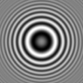
However, one is only able to measure the absolute value and not the complex valued amplitude. After simplification, the problem of reconstruction of a diffraction pattern from objects in the $z_{j}$-plane can be modelled as deconvolution with the following kernel, see Figure 1

$$\kappa_{z_{j}}(x,y)=h_{z_{j}}(x,y)=\frac{\sin(\tfrac{\pi}{\lambda z_{j}}(x^{2}+y^{2}))}{\lambda z_{j}}.$$

Figure 1: Left: Convolution kernel $\kappa$ for digital holography $\lambda=630$nm and recording distance of 250mm. Right: Simulated hologram with 20 particles.

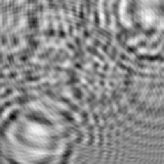
We generated a hologram $g$ with a number of particles all located in the same plane. Then we applied the projection proximal-point algorithm to the solution of the inverse problem with the operator

$$Ku=\kappa_{z_{j}}\ast u.$$

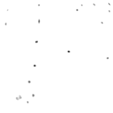
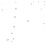
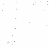
We show reconstruction of the objects with different methods in Figure 2. Note that all methods delivered well seperated and moderately sharp objects. However, the result for the projection proximal-point algorithm with generalized conditional gradient method gives a slightly sharper reconstruction.

ppp, soft thresholding	soft thresholding
ppp, gen. cond. grad	hard thresholding

Figure 2: Reconstructions of the hologram from Figure 1 with different methods and 120 iterations. Top left: Projection proximal-point method with damped soft thresholding in the inner loop. Top right: Iterated soft thresholding [7]. Bottom left: Projection proximal-point method with generalized conditional gradient method (Algorithm 3) in the inner loop. Bottom right: Iterated hard thresholding [3].

In Figure 3 the development of the functional value is shown. We remark, that the projection proximal-point algorithm does not necessarily reduce the functional value and sometimes, depending on the problem and the parameters, does not produce monotonically decaying objective values. However, this may be an advantage of the algorithms since it does not have to follow a decent direction. Note that iterated hard-thresholding (which is also a generalized conditional gradient method) performs worst and that the iterated soft-thresholding alone or in combination with the proximal-point modification behave better and somewhat similar. However, combining the generalized conditional gradient method with the proximal-point modification gives significant improvement.

Figure 3: Decay of the functional value for the problem of digital holoraphy example and different methods. The parameters are similar toFigure 2.

5.2 Deblurring and the influence of $\mu$ and $\sigma$

The parameters $\mu$ and $\sigma$ influence the behavior of the algorithm. Basicallly, the parameter $\mu$ influences how much the subproblems are regularized and hence, for larger values of $\mu$ the subproblems are solved faster, see, e.g. the rate of convergence in Theorem 3.1. The parameter $\sigma$ tunes the desired accuracy for the subproblems, i.e. the smaller $\sigma$ is, the more accurate is the solution of the subproblem and hence, the subproblems are solved slower. As a rule of thumb one may remember that it does not seem necessary to choose $\sigma$ too small, i.e. it is enough to solve the subproblems only roughly. Typically $\sigma=0.9$ is a good choice. On the other hand, not too much regularization is necessary to terminate the inner loop quickly, i.e. small values of $\mu$ give good results. A typical value for may be $\mu=0.05$. Moreover, smaller $\mu$ often lead to faster decay of the functional value in the experiments.

To illustrate this behaovior we performed a one dimensional deconvolution experiment. We considered a discretized linear blurring operator $A$ which consisted of the circular convolution with the kernel $\kappa(x)=1/(1+x^{2}/5^{2})$ and combinded this with a synthesis operator $B$ associated with simple hat-functions and hence, considered the operator $K=AB$. We generated data which just consists of a few spikes and hence, has a sparse representation in hat functions. We ran the projection proximal-point algorithm (Algorithm 4) with different values for $\mu$ and $\sigma$ and with both soft-thresholding (Algorithm 2) and the generalized conditional gradient method (Algorithm 3) in the inner loop. The decay of the objective value as shown in Figure 4 and 5 is typical.

Figure 4: Decay of the functional value for the projection proximal-point algorithtm with soft-thresholding in the inner loop for the deconvolution problem and different values of $\sigma$ and $\mu$.

Figure 5: Decay of the functional value for the projection proximal-point algorithm with the generalized conditional gradient method in the inner loop for the deconvolution problem and different values of $\sigma$ and $\mu$.

To get an impression, how the values of the parameter $\mu$ and $\sigma$ influence the termination of the inner loop due to conditons (11)–(13), we recorded the numbers of inner and outer iterations for different values of $\mu$ and $\sigma$ in Table 5.2 for soft thresholding and in Table 5.2 for the generalized conditional gradient method. In all cases we ran the algorithm until 350 total iterations have been done. (Note that this sometimes causes that the last inner iteration did not terminate, see e.g. Table 5.2 bottom left). First one notes that smaller values of $\sigma$ cause the inner iteration to take longer to terminate and the same holds true for smaller values of $\mu$. Moreover, we see that smaller values of $\sigma$ (i.e. solving the subproblems more precise) does not improve the decay of the functional value. Hence, we may conclude, that a larger value of $\sigma$ is preferable in general. The value of $\mu$ behaves differently for soft-thresholding and the generalized conditional gradient method. While for the first, smaller values of $\mu$ lead to better results concerning the functional value, for the latter the converse holds true. Finally, the generalized conditional gradient method gives in general smaller functional values.

$\mu=0.2$, $\sigma=0.1$

$\mu=0.2$, $\sigma=0.9$

& # out iter # in inter $\Psi(u^{n})$ 1 1 8.88e-02 2 1 5.20e-02 3 1 3.68e-02 ⋮ ⋮ ⋮ 347 1 1.46e-03 348 1 1.46e-03 349 1 1.46e-03 350 1 1.46e-03 $\mu=0.01$, $\sigma=0.1$ $\mu=0.01$, $\sigma=0.9$ # out iter # in inter $\Psi(u^{n})$ 1 101 5.06e-03 2 190 2.06e-03 # out iter # in inter $\Psi(u^{n})$ 1 6 2.08e-01 2 11 1.49e-01 3 12 9.76e-02 ⋮ ⋮ ⋮ 16 14 1.70e-03 17 14 1.63e-03 18 13 1.58e-03 19 13 1.54e-03

Table 1: Output of the projection proximal-point algorithm with soft thresholding in the inner loop. The problem under consideration in the deblurring problem.

& # out iter # in inter $\Psi(u^{n})$ 1 1 1.54e-01 2 1 7.78e-02 3 1 4.36e-02 ⋮ ⋮ ⋮ 347 1 1.10e-03 348 1 1.10e-03 349 1 1.10e-03 350 1 1.10e-03 $\mu=0.01$, $\sigma=0.1$ $\mu=0.01$, $\sigma=0.9$ # out iter # in inter $\Psi(u^{n})$ 1 27 4.59e-03 2 32 1.97e-03 3 85 1.60e-03 4 83 1.44e-03 5 1 1.33e-03 6 12 1.27e-03 7 97 1.22e-03 8 1 1.19e-03 # out iter # in inter $\Psi(u^{n})$ 1 5 1.84e-01 2 4 5.94e-02 3 4 2.51e-02 ⋮ ⋮ ⋮ 56 3 1.03e-03 57 6 1.05e-03 58 44 1.02e-03 59 1 1.01e-03

Table 2: Output of the projection proximal-point algorithm with the generalized conditional gradient method in the inner loop. The problem under consideration in the deblurring problem.

6 Conclusion

The projection proximal point algorithm as proposed in [20] is applicable for the problem of $\ell^{1}$-minimization. It could be shown that under the FBI assumption the algorithm even converges linearly. Both the iterated soft-thresholding and the generalized conditional gradient method are applicable methods to solve the regularized subproblems. For the iterated soft-thresholding the projection proximal-point algorithm does not lead to a significant improvement. On the theoretical side, the iterated soft-thresholding itself converges linearly [4, 14] and on the practical side, both methods behave comparable (see Figure 3). However, for the generalized conditional gradient method the situation is different. For the algorithm itself as stated in [3] the distance to the minimizer only converges like $\mathcal{O}(n^{-1/2})$ but the projection proximal-point extension gives linear convergence. Moreover, also the practical behavior is better, see Figure 3. In total, it seems that the generalized conditional gradient method combines well with the projection proximal point idea.

However, the aim of this paper was not to develop the fastest available method for $\ell^{1}$-minimization but to provide an algorithm from a different class of methods. Hence, it may be expected that after considerable fine tuning (parameter choice rules, more efficient solvers for the subproblems, backtracking,…) the projection proximal-point algorithm will become comparable to state-of-the-art methods.

Finally we remark, that Algorithm 4 does not rest upon linearity of the operator and may also be applied to non-linear operators. Also for the solution of the subproblems either iterated soft-thresholding [1] or the generalized condition gradient method may be used.

References

- [1] Thomas Bonesky, Kristian Bredies, Dirk A. Lorenz, and Peter Maass. A generalized conditional gradient method for nonlinear operator equations with sparsity constraints. Inverse Problems, 23:2041–2058, 2007.
- [2] Andrea Braides. -convergence for Beginners. Oxford Lecture Series in Mathematics and Its Applications. Oxford University Press, 2002.
- [3] Kristian Bredies and Dirk A. Lorenz. Iterated hard shrinkage for minimization problems with sparsity constraints. SIAM Journal on Scientific Computing, 30(2):657–683, 2008.
- [4] Kristian Bredies and Dirk A. Lorenz. Linear convergence of iterative soft-thresholding. Journal of Fourier Analysis and Applications, 14(5–6):813–837, 2008.
- [5] Kristian Bredies, Dirk A. Lorenz, and Peter Maass. A generalized conditional gradient method and its connection to an iterative shrinkage method. Computational Optimization and Applications, 42(2):173–193, 2008.
- [6] Patrick L. Combettes and Valérie R. Wajs. Signal recovery by proximal forward-backward splitting. Multiscale Model. Simul., 4(4):1168–1200, 2005.
- [7] Ingrid Daubechies, Michel Defrise, and Christine De Mol. An iterative thresholding algorithm for linear inverse problems with a sparsity constraint. Communications in Pure and Applied Mathematics, 57(11):1413–1457, 2004.
- [8] Loïc Denis, Dirk A. Lorenz, and Dennis Trede. Greedy solution of ill-posed problems: Error bounds and exact inversion. Preprint 8, DFG SPP 1324, arXiv:0904.0154, 2009.
- [9] David L. Donoho and Yaakov Tsaig. Fast solution of -norm minimization problems when the solution may be sparse. IEEE Transactions on Information Theory, 54(11):4789–4812, 2008.
- [10] Bradley Efron, Trevor Hastie, Iain M. Johnstone, and Robert Tibshirani. Least angle regression. The Annals of Statistics, 32(2):407–451, 2004.
- [11] Mário A. T. Figueiredo, Robert D. Nowak, and Stephen J. Wright. Gradient projection for sparse reconstruction: Applications to compressed sensing and other inverse problems. IEEE Journal of Selected Topics in Signal Processing, 4:586–597, 2007.
- [12] Joseph W. Goodman. Introduction to Fourier optics. Roberts & Co, 2005.
- [13] Roland Griesse and Dirk A. Lorenz. A semismooth Newton method for Tikhonov functionals with sparsity constraints. Inverse Problems, 24(3):035007 (19pp), 2008.
- [14] Elaine T. Hale, Wotao Yin, and Yin Zhang. Fixed-point continuation for -minimization: Methodology and convergence. SIAM Journal on Optimization, 19(3):1107–1130, 2008.
- [15] Klaus D. Hinsch. Three-dimensional particle velocimetry. Measurement Science and Technology, 6(6):742–753, 1995.
- [16] Klaus D. Hinsch and Sven F. Hermann. Holographic particle image velocimetry. Measurement Science and Technology, 13(7):61–72, 2002.
- [17] Seung-Jean Kim, Kwangmoo Koh, Michael Lustig, Stephen Boyd, and Dimitry Gorinevsky. A method for large-scale -regularized least squares problems with applications in signal processing and statistics. IEEE Journal on Selected Topics in Signal Processing, 1(4):606–617, 2007.
- [18] Thomas Kreis. Handbook of holographic interferometry: optical and digital methods. Wiley, 2005.
- [19] Michael R. Osborne, Brett Presnell, and Berwin A. Turlach. A new approach to variable selection in least squares problems. IMA Journal of Numerical Analysis, 20:389–404, 2000.
- [20] Mikhail V. Solodov and Benar F. Svaiter. A hybrid projection-proximal point algorithm. Journal of Convex Analysis, 6(1):59–70, 1999.
- [21] Ferrél Soulez, Loïc Denis, Éric Thiébaut, Corinne Fournier, and Charles Goepfert. Inverse problem approach in particle digital holography: out-of-field particle detection made possible. Journal of the Optical Society of America A, 24(12):3708–3716, 2007.
- [22] Ferréol Soulez, Loïc Denis, Corinne Fournier, Éric Thiébaut, and Charles Goepfert. Inverse problem approach for particle digital holography: accurate location based on local optimisation. Journal of the Optical Society of America A, 24(4):1164–1171, 2007.
- [23] Chandra S. Vikram. Particle field holography. Cambridge University Press, 1992.