Surface tension fluctuations and a new spinodal point in glass-forming liquids

The dramatic slowdown of glass-forming liquids review:angell88 has been variously linked to increasing dynamic heterogeneities:berthier05 ; review:ediger00 and static self:prl07 ; self:nphys08 correlation lengths. Yet, empirical evidence is insufficient to decide among competing theories glassthermo:gibbs58 ; mosaic:kirkpatrick89 ; glassthermo:mezard99 ; heterogeneities:garrahan02 ; review:tarjus05 ; glassthermo:moore06 . The random first-order theory (RFOT) mosaic:kirkpatrick89 links the dynamic slowdown to the growth of amorphous static order, whose range depends on a balance between configurational entropy and surface tension. This last quantity is expected to vanish when the temperature surpasses a spinodal point beyond which there are no metastable states. Here we measure for the first time the surface tension in a model glass-former, and find that it vanishes at the energy separating minima from saddles, demonstrating the existence of a spinodal point for amorphous metastable order. Moreover, the fluctuations of surface tension become smaller for lower temperatures, in quantitative agreement with recent theoretical speculation self:nphys08 that spatial correlations in glassy systems relax nonexponentially because of the narrowing of the surface tension distribution.

It is only recently that a static correlation length $\xi$ has been clearly detected in a glassforming liquid self:prl07 ; self:nphys08 , by measuring a point-to-set correlation function mosaic:bouchaud04 ; dynamics:montanari06 . The idea is to consider a liquid region of size $R$ subject to amorphous boundary conditions provided by the surrounding liquid frozen into an equilibrium configuration. The external particles act as a pinning field favouring internal configurations which best match the frozen exterior. Clearly, the effect of the border on the innermost part of the region is smaller as $R$ grows larger. Less trivially, on lowering the temperature the effect of the amorphous boundary conditions propagates deeper into the region. More precisely, if we measure some correlation (or overlap) $q_{c}(R)$ between the initial configuration of the region and that reached at infinite time under the effect of the amorphous boundary conditions, the decay of $q_{c}(R)$ is slower the lower $T$ self:prl07 ; self:nphys08 . This demonstrates the existence of an increasing static correlation length $\xi$. Irrespective of its precise definition, $q_{c}(R)$ is the point-to-set correlation function.

According to RFOT, the decay of $q_{c}(R)$ is regulated by competition between a surface energy cost, $YR^{\theta}$, trying to keep the region to the same amorphous state as the external configuration, and a configurational entropy gain, $T\Sigma R^{d}$, favouring a transition to another of the exponentially many states, ${\cal N}(R)\sim\exp(R^{d}\Sigma)$, available to the region self:prl07 . The surface tension $Y$ is predicted to vanish for temperatures higher than a spinodal value. Above this point metastable states merge into a single ergodic state. The cost/gain terms balance at $R=\xi\equiv(Y/T\Sigma)^{\frac{1}{d-\theta}}$: for $R<\xi$ the surface cost $Y_{c}R^{\theta}$ keeps the region in the same state as the external environment; for $R>\xi$ the entropic gain $T\Sigma R^{d}$ dominates and the region is free to rearrange into some other state. The RFOT length $\xi$ is not only the typical size of the rearranging regions; it also represents the largest scale over which it is sensible to define a metastable state: a state defined over a region much larger than $\xi$ is unstable against fragmentation into sub-regions of typical scale $\xi$. For this reason RFOT is also called mosaic theory.

The existence of many metastable states is central to RFOT. But for more than one state to exist, a nonzero surface tension is necessarily required. In fact, one may argue that the surface tension is as much a fundamental ingredient of the theory as the configurational entropy, if not more. Hence a direct empirical investigation of the surface tension is needed in order to put a more stringent test on RFOT. This is what we do here.

Surface tension is defined as the free energy cost per unit area associated to a surface separating two phases review:navascues79 . The determination of the surface free energy between metastable states is very challenging, first, because metastable states are amorphous and the interfaces are hard to detect, and second, because their lifetime is necessarily finite. Excitations are constantly forming and relaxing: this is the relaxation mechanism of RFOT, through which the whole liquid state is slowly explored. For our initial study of surface tension we choose to avoid such complications and focus on inherent structures, i.e. local minima of the potential energy landscape:stillinger84 . This approach measures energy rather than free energy, so we expect our results to apply quantitatively only at quite low temperatures.

We consider a set of ISs obtained minimizing equilibrated instantaneous configurations of a model soft-sphere glassformer (see Methods). Our lowest working temperature is $T=0.89\,T_{c}$ ($T_{c}$ is the Mode Coupling temperature rev:goetze_leshouches1987 )

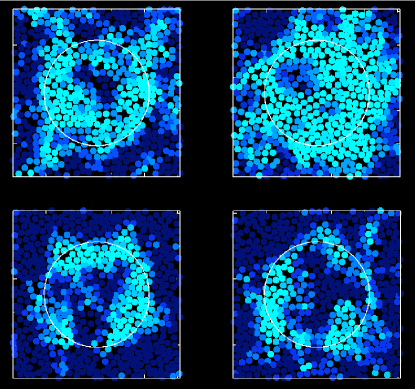
Given a pair $\alpha$ and $\beta$ of ISs, we exchange between them all particles located within a sphere of radius $R$. We then minimize the two configurations thus obtained to produce two new ISs. Each of them is a hybrid minimum, resembling the “parent” minima far from the surface of the sphere but rearranged close to it (Fig. 1).

Figure 1: Map of the excitation. Overlap, i.e. similarity, between the configuration right after the exchange of the spheres and the hybrid inherent structure after minimization. Only a thin slice located at half height of the whole three dimensional system is shown. Each particle is coloured according to how much it moved after the artificial excitation was created (dark blue: small displacement, high overlap — ligth blue: large displacement, small overlap). Upper panel: two configurations at high temperature $T=1.33\,T_{c}$. Lower panel: two configurations at low temperature $T=0.89\,T_{c}$. The hybrid minimum clearly bears memory (high overlap, dark blue) of the parent ISs far from the boundary of the sphere (white circle). On the other hand, the memory is lower (low overlap, light blue) along the interface, where particles have been moved the most by the minimization procedure. Although at lower temperature the interface is somewhat sharper, it is in general quite rough. Strong fluctuations of the overlap along the interface are evident, clearly indicating that there are large surface tension fluctuations. Note that the hybrid configuration is nevertheless a typical IS of the system: the only reason why we can visualize the interface is that we know a priori the shape and position of the excitation and we can use the parent configurations as reference to calculate overlap. Without this information, it would be impossible to distiguish the hybrid inherent structure from any other one.

For each hybrid IS we compute the surface energy $E^{\text{s}}_{\alpha\beta}$ by subtracting the parent ISs’ contribution (see Methods). Fig. 2 shows the sample-averaged surface energy, $E^{\text{s}}$, vs. $R$ for several temperatures. There is a well-defined relationship between surface energy and size, regulated by the temperature: at fixed $R$, $E^{\text{s}}$ increases by decreasing $T$. The data do not correspond to a single power-law scaling, so we propose

$$E^{\text{s}}=Y_{\infty}R^{\theta}-\delta R^{\omega},$$ (1)

where $Y_{\infty}$ is the asymptotic surface tension and $\omega<\theta$. The subleading $\delta R^{\omega}$ correction is quite natural. It is present in liquids (with $\omega=1$) due to curvature effects review:navascues79 , and in disordered systems, where it may arise either from bulk contributions, as in the random field Ising model tension:imry75 , or from interface roughening that lowers the surface energy, as in the random bond Ising model tension:halpin95 .

Figure 2: Surface energy. $E^{\text{s}}$ as a function of the excitation radius $R$ at various temperatures. A single power law fit $R^{\theta}$ would give an exponent $\theta>2$, which is hard to justify. On the other hand, especially at high $T$ it is clear that there are small $R$ corrections to a single power law. Full lines are fits using equation (1), with $\theta=2$ and $\omega=1.5$. Dotted lines show as a reference the power laws with $\theta=2$ and $\theta=3/2$. Error bars are smaller than symbol size.

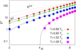
We must choose the exponents of eq. (1) with some criterion, because the nonlinear fit with four parameters is marginally stable, and many sets of parameters give good fits. Our data strongly suggest the conservative choice $\theta=2$, which seems to describe the large $R$ behaviour better than the alternative $\theta=3/2$ predicted by a wetting argument mosaic:xia00 ; mosaic:dzero05 . The value $\theta=2$ is also found in spin models with finite range interactions nucleation:franz05 . To fix $\omega$, we take eq. (1) as valid for the whole population of surface energies (instead of just the average), and ascribe all fluctuations of $E^{\text{s}}_{\alpha\beta}$ to the quantity

$$\delta_{\alpha\beta}=\frac{Y_{\infty}R^{2}-E^{\text{s}}_{\alpha\beta}}{R^{\omega}}.$$ (2)

We then require that the variance of $\delta_{\alpha\beta}$ be independent of $R$, which is the typical behaviour of random systems tension:huse85 ; tension:halpin95 . This procedure (see Methods) gives $\omega=1.5(2)$.

With $\theta$ and $\omega$ thus fixed, eq. (1) fits the $E^{\text{s}}(R)$ data very well (Fig. 2), and we obtain the asymptotic surface tension $Y_{\infty}$ as a function of $T$ (Fig. 3, top). We find that $Y_{\infty}$ decreases for higher $T$, and becomes quite small above $T_{c}$. Yet, the decrease is rather smooth, so that it is hard to define a spinodal temperature.

Figure 3: Surface tension vs. temperature. Upper panel: $Y_{\infty}$ as a function of the quenching temperature of the inherent structures. The vertical dotted line marks the mode coupling temperature. The surface tension decreases on increasing $T$, although too smoothly to indicate a sharp spinodal temperature. Lower panel: inherent structure energy as a function of the quenching temperature. A comparison of the two curves clearly shows that they are correlated.

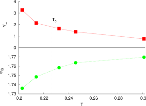
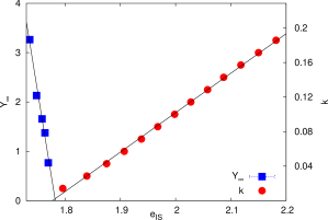
On the other hand, the plot of the average IS energy, ${e_{\text{IS}}}$, vs. $T$ (Fig. 3, bottom) suggests using the energy as a control parameter. Indeed, the $Y_{\infty}$ vs. ${e_{\text{IS}}}(T$) curve is nearly linear (Fig. 4, left), indicating that $Y_{\infty}$ vanishes quite sharply at a well-defined energy ${e_{\text{th}}}$. Interestingly enough, ${e_{\text{th}}}$ is very close to the threshold, i.e. the energy below which minima start to dominate the energy landscape self:prl02 ; self:jcp06 . The threshold ${e_{\text{th}}}$ is defined as the point where the instability index of saddles vanishes (Fig. 4, right). Hence ${e_{\text{th}}}$ is the true spinodal point of amorphous order, fixing the upper limit of stability of the RFOT mechanism.

Figure 4: The spinodal point. Left: $Y_{\infty}$ (squares) vs. IS energy. Right: intensive saddle instability index $k$ (circles) vs. IS energy. Lines are linear fits to the data. Both the surface tension and the instability index seem to vanish at a similar energy, the threshold ${e_{\text{th}}}$, which is therefore the spinodal point. Instability index data are from ref. self:jcp06, .

We expect the surface tension to fluctuate when considering different pairs of ISs. We thus compute the distribution of the single-sample surface tension,

$$Y_{\alpha\beta}\equiv\frac{E^{\text{s}}_{\alpha\beta}}{R^{2}}.$$ (3)

The distribution $P(Y,R,T)$ for two values of $R$ is shown in Fig. 5. The first thing we notice is that the distribution is quite broad. This means that the original RFOT, which assumed a sharp value of $Y$, cannot hold strictly. If there is a single surface tension, a region smaller than $\xi$ cannot rearrange, so that a nonfluctuating surface tension implies a sharp drop of the point-to-set correlation $q_{c}(R)$ at $R\sim\xi$. With a fluctuating surface tension, on the other hand, any region can decorrelate, as long as there are target states with surface tension $Y<T\Sigma R^{d-\theta}$. Our finding is thus consistent with the smooth decay of the correlation observed numerically self:prl07 ; self:nphys08 .

Figure 5: Surface tension distribution. Normalized histograms of the surface tension for $T=0.89\,T_{c}$ at two values of $R$. Note that this distribution does not depend on the exponent $\omega$ and that its average tends to $Y_{\infty}(T)$ for $R\to\infty$. The distribution narrows on increasing $R$, and thus on lowering the temperature. Solid lines correspond to fits with the Weibull distribution $P(Y)=-d/dY\exp[-(Y/y_{c})^{\hat{\zeta}}]$ (see Ref. self:nphys08, ). Inset: variance of $Y_{\alpha\beta}$ vs. $R$. For small $R$ this quantity seems to decay as $1/R^{2}$, but at larger $R$ it is clearly larger. Note that that, $\text{Var}[Y_{\alpha\beta}]=\text{Var}[Y_{\infty}]+\text{Var}[\delta_{\alpha\beta}]/R^{4-2\omega}$. If $\text{Var}[\delta_{\alpha\beta}]$ does not depend on $R$ and $\omega\sim 3/2$, then $\text{Var}[\delta_{\alpha\beta}]/R^{4-2\omega}\sim 1/R$, which is compatible with the large $R$ behaviour of the data.

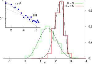
The second important result is that the distribution narrows as $R$ grows. To interpret this correctly, note that $P(Y)$ depends on $T$ both directly through the quench temperature of the ISs and indirectly through $R$. Since the only relevant lengthscale is $\xi(T)$, the typical size of the rearranging regions, we can define

$$P(Y,T)\equiv P(Y,R=\xi(T),T),$$ (4)

where $\xi(T)$ is taken from simulations self:nphys08 . When $T$ decreases, $\xi(T)$ grows, $P(Y,T)$ narrows, and the decay of $q_{c}(R,T)$ sharpens. This is indeed the numerical finding self:nphys08 : the decay is well described by a compressed exponential,

$${q_{c}}(R,T)\sim\exp\left[{-(R/\xi)}^{\zeta}\right],$$ (5)

where the anomaly $\zeta$ grows from $1$ at high temperature up to $\sim 4$ at low $T$ (higher $\zeta$ means sharper decay). The link between $P(Y,T)$ and sharpness of decay can be made more quantitative. The overlap ${q_{c}}(R)$ is given by self:nphys08

$${q_{c}}(R,T)=\int_{T\Sigma R^{d-\theta}}^{\infty}P(Y,T;R)\,dY.$$ (6)

Using the approximation (4) (see Methods) and defining $y=T\Sigma R^{d-\theta}$ we obtain

$$\hat{q}_{c}(y,T)=\int_{y}^{\infty}\!\!\!\!P(Y,T)\,dY.$$ (7)

In this way we avoid the complexity $\Sigma$, whose estimate is always very tricky self:coluzzi99 . If eq. (5) holds, we must have a similar compressed exponential form, $\hat{q}_{c}\sim\exp[-(y/y_{c})^{\hat{\zeta}}]$, with the two anomalies related by $\hat{\zeta}=\zeta/(d-\theta)$. We computed $\hat{q}_{c}(y,T)$ at the lowest temperature, $T=0.89\,T_{c}$, where the the difference between energy and free energy should be less harmful. A compressed exponential fit gives $\zeta\approx 4.2(1)$, encouragingly close to the value $\zeta=4.0(6)$ of ref. self:nphys08, . The agreement on the values of $\zeta$ found with two completely different protocols puts the generalized RFOT on a firmer basis.

The present study provides independent evidence of the existence of a surface tension distribution with the properties required by a generalized RFOT, and it thus supports its validity as a description of deeply supercooled liquid. The fact that $P(Y,T)$ broadens and clusters around $Y\sim 0$ for $T\gtrsim T_{c}$, (i.e. for $E\geq E_{th}$) is significant in two ways. First, it implies a crossover from many states to one state through a spinodal mechanism: a null surface energy cost means that rearrangements are no longer excitations. Secondly, it says that this transition is smooth: instead of disappearing abruptly at $T_{c}$ (as in mean-field self:castellani05 ) metastable states slowly “fade out”, because excitations are becoming less and less costly on average and because states are slowly merging with each other, as indicated by many pairs of states having near-zero surface tension.

Methods

System.

We have simulated a three dimensional soft-sphere binary mixture soft-spheres:bernu87 using Metropolis Monte Carlo with particle swaps self:pre01 . The pair potential is $v_{ij}(\mathbf{r}_{i},\mathbf{r}_{j})=[(\sigma_{i}+\sigma_{j})/|\mathbf{r}_{i}-\mathbf{r}_{j}|]^{12}$, with a polynomial smooth cut-off at large distances (parameters as given in Ref. self:nphys08, ). The mode-coupling temperature for this system is $T_{c}=$0.226 soft-spheres:roux89 . A system of $N=16384$ particles was considered in a box of lenght $25.4$ (in such units the number density is $1$).

Minimization.

Minimization of instantaneous configurations was done with the LBFGS algorithm algorithm:liu89 . After exchanging the particles of the sphere, some pairs of particles end up at very short distances, giving very high energies and gradients that tend to destabilize the minimizer. For these configurations, we have minimized with a combination of $100$ standard Metropolis Monte Carlo steps at $T=0$ plus LBFGS. The sphere is placed so that the density and composition of the resulting configurations are identical to those of the initial ISs.

Definition of surface energy.

We indicate with $E_{\alpha\beta}$ and $E_{\beta\alpha}$ the energies of the hybrid configurations. The first label indicates the original parent configuration outside the sphere. The surface energy is

$$E^{\text{s}}_{\alpha\beta} =E_{\alpha\beta}-E^{\text{int}}_{\beta}-E^{\text{ext}}_{\alpha},$$ (8)

$$E^{\begin{subarray}{c}\text{ext}\\ \text{int}\end{subarray}} =\sum_{i,j:|\mathbf{r}_{i}|\gtrless R}v_{ij}(\mathbf{r}_{i}-\mathbf{r}_{j})\ .$$ (9)

The exponent $\omega$.

Our estimation of $\omega$ relies on the physical hypothesis that the prefactor $\delta$ in the correction term of Eq. (1) (unlike $Y_{\infty}$) has large fluctuations even for $R\to\infty$. This behaviour is rather ubiquitous in disordered media tension:halpin95 ; tension:huse85 ; tension:imry75 and finds some confirmation here by the violation of the central limit theorem shown by the variance of $Y_{\alpha\beta}$ at large $R$ (see Fig. 5, inset). We fix $\omega$ at the value for which the variance $\text{Var}[\delta(\omega)]$ is independent of$R$ with the following self-consistent procedure: for a running value of the exponent, $\tilde{\omega}$, we fit the average of $E_{s}$ via Eq. (1) to obtain $Y_{\infty}(\tilde{\omega})$ and a variance $\text{Var}[\delta(\tilde{\omega})]$. At large $R$

$$\text{Var}[E_{s}]\sim\text{Var}[\delta(\tilde{\omega})]R^{2\tilde{\omega}},$$ (10)

where $\text{Var}[\tilde{\omega}]$ will in general depend on $R$. A similar formula holds for $\tilde{\omega}=\omega$, but with $R$-indepdent variance, so that

$$\log\text{Var}[\delta(\tilde{\omega})]=\log\text{Var}[\delta(\omega)]+2(\omega-\tilde{\omega})\log R.$$ (11)

The procedure is to fit $\log\text{Var}[\delta]$ vs. $\log R$ for several values of $\tilde{\omega}$ to obtain a slope $a(\tilde{\omega})$ which is finally fitted to $a(\tilde{\omega})=2(\omega-\tilde{\omega})$ to obtain $\omega$. When we do this we do not find any trend of $\omega$ with the temperature. Thus, to get rid of unwanted thermal noise in the determination of this exponent we use the lowest $T$ to fix its value. This procedure gives $\omega=1.5(2)$, which is very much within the range of values provided by nonlinear fit of the data surface energy with all four parameters free.

Calculation of the anomaly.

The distribution $P(Y;R)$ is peak-shaped in $Y$; as $R$ is increased the peak narrows and shifts to the right, approaching $Y_{\infty}$. Eq. (6) says that the overlap is the area of $P(Y;R)$ to the right of $T\Sigma R$. Around $\xi$, ${q_{c}}(R)$ is rapidly decaying, so that $T\Sigma R$ must be greater than the peak position for all $R>\xi$, and the integral is just measuring the area of the right tail of $P(Y;R)$. To study the shape of ${q_{c}}(R)$ near the inflection point $\xi$ (which dominates the value of $\zeta$), we may thus approximate $P(Y;R)$ with $P(Y;\xi)$ (with the consequence of slightly overestimating the sharpness of the decay).

The minimal energy with frozen environment.

We have treated the external and the internal parts of the spherical excitations symmetrically. However, one may argue that when a region rearranges, it chooses the target state with the minimum energy with respect to the external environment (S. Franz, private communication). This is certainly the case in the numerical experiments of ref. self:nphys08, , where the amorphous boundary of the rearranging region is really frozen. We therefore define the minimal surface energy at fixed external IS,

$$E^{\text{s}}_{\beta_{0},\alpha}=\min_{\beta}\{E_{\alpha\beta}\}-E^{\text{ext}}_{\alpha}-E^{\text{int}}_{\beta_{0}},$$ (12)

where $\beta_{0}$ is the $\beta$ that minimizes $E_{\alpha\beta}$. From this minimum surface energy at fixed $\alpha$, we can obtain the distribution $P_{0}(Y)$ by varying the external IS $\alpha$. This $P_{0}(Y)$ is the distribution that must be plugged into the generalized RFOT expression for the overlap, (6), to get $\zeta$. The value of the anomaly obtained in this way is $\zeta\approx 4.4$, comparable to the value $\zeta\approx 4.2$ found with $P(Y)$. Indeed, apart form the poorer statistics that makes $P_{0}(Y)$ considerably more noisy than $P(Y)$, the form of the two distributions is very similar.