Addressing the bias in Monte Carlo pricing of multi-asset options with multiple barriers through discrete sampling

Abstract

An efficient conditioning technique, the so-called Brownian Bridge simulation, has previously been applied to eliminate pricing bias that arises in applications of the standard discrete-time Monte Carlo method to evaluate options written on the continuous-time extrema of an underlying asset. It is based on the simple and easy to implement analytic formulas for the distribution of one-dimensional Brownian Bridge extremes. This paper extends the technique to the valuation of multi-asset options with knock-out barriers imposed for all or some of the underlying assets. We derive formula for the unbiased option price estimator based on the joint distribution of the multi-dimensional Brownian Bridge dependent extrema. As analytic formulas are not available for the joint distribution in general, we develop upper and lower biased option price estimators based on the distribution of independent extrema and the Fréchet lower and upper bounds for the unknown distribution. All estimators are simple and easy to implement. They can always be used to bind the true value by a confidence interval. Numerical tests indicate that our biased estimators converge rapidly to the true option value as the number of time steps for the asset path simulation increases in comparison to the estimator based on the standard discrete-time method. The convergence rate depends on the correlation and barrier structures of the underlying assets.

Key Words: Monte Carlo simulation, extreme values, Brownian Bridge, multi-asset barrier option, multi-variate joint distribution, Fréchet bounds.

1 Introduction

Barrier options introduced by Merton (1973) are used widely in trading now. The option is extinguished (knocked-out) or activated (knocked-in) when an underlying asset reaches a specified level (barrier). A lot of related more complex instruments for example bivariate barrier, ladder, step-up or step-down barrier options have become very popular in over-the-counter markets. In general, these options can be considered as options with payoff depending upon the path extrema of the underlying assets. A variety of closed form solutions for such instruments on a single underlying asset have been obtained in the classical Black-Scholes settings of constant volatility, interest rate and barrier level. See for example Heynen and Kat (1994a), Kunitomo and Ikeda (1992), Rubinstein and Reiner (1991). If the barrier option is based on two assets then a practical analytical solution can be obtained for some special cases considered in Heynen and Kat (1994b) and He, Keirstead and Rebholz (1998).

In practice, however, numerical methods are used to price the barrier options for a number of reasons, for example, if the assumptions of constant volatility and drift are relaxed or payoff is too complicated. Numerical schemes such as binomial and trinomial lattices (Hull and White (1993), Kat and Verdonk (1995)) or finite difference schemes (Dewynne and Wilmott (1993)) can be applied to the problem. However, the implementation of these methods can be difficult. Also, if more than two underlying assets are involved in the pricing equation then these methods are not practical.

In this paper we focus on a Monte Carlo simulation method which is a good general pricing tool for such instruments. However, finding the extrema of the continuously monitored assets by sampling assets at discrete dates, the standard discrete-time Monte Carlo approach, is computationally expensive as a large number of sampling dates and simulations are required. Loss of information about all parts of the continuous-time path between sampling dates introduces a substantial bias for the option price. The bias decreases very slowly as $1/\sqrt{M}$ for $M>>1$, where $M$ is the number of equally spaced sampling dates (see Broadie, Glasserman and Kou (1997)). Also, extrapolation of the Monte Carlo estimates to the continuous limit is usually difficult due to finite sampling errors. For the case of a single underlying asset, it was shown by Andersen and Brotherton-Ratcliffe (1996) and Beaglehole, Dybvig and Zhou (1997) that the bias can be eliminated by a simple conditioning technique, the so-called Brownian Bridge simulation. The method is based on the simulation of a one-dimensional Brownian bridge extremum between the sampled dates according to a simple analytical formula for the distribution of the extremum. The technique is very efficient because only one time step is required to simulate the asset path and its extremum if the barrier, drift and volatility are constant over the time region. We extend the technique to the valuation of multi-asset options with continuously monitored knock-out barriers imposed for some or all underlying assets. We derive the general formula for the unbiased estimator based on the joint distribution of the multi-dimensional Brownian Bridge dependent extrema. In general, however, the analytic formulas are not available for this joint distribution and we develop three biased estimators. The upper and lower estimators are based on the Fréchet bounds for the unknown multi-variate joint distribution of the extrema. The third estimator (which is typically most accurate) is based on the joint distribution of the independent extrema. The biased estimators can be used to bind the true option price by a confidence interval. Numerical examples indicate that the biases rapidly decrease as $M$ increases in comparison to the bias in the standard discrete-time method and the convergence rate depends on the correlation and barrier structures of the underlying assets. Finally we discuss the application of our biased estimators for the valuation of knock-in, cash-at-hit rebates options, lookback options and credit derivatives.

2 Unbiased estimator via Brownian Bridge correction

2.1 Model setup

Consider the knock-out option $Q$ written on the underlying assets $\vec{S}(t)=(S_{1}(t),...,S_{d}(t))$. The option payout at maturity $t=T$ is some function $V(\vec{S}(T))$ if the underlying assets never hit the fixed boundaries $\vec{h}(t)<\vec{S}(t)<\vec{H}(t),\;\;t\in[0,T]$ and zero otherwise. Here $\vec{H}(t)=(H_{1}(t),...,H_{d}(t))$ and $\vec{h}(t)=(h_{1}(t),...,h_{d}(t))$ are the upper and lower barriers. Hereafter, we use vector notation to simultaneously compare all vector components. For example, $\vec{A}<\vec{B}$ is used to denote $A_{i}<B_{i}$ for all $i=1,...,d$.

Assume that the underlying assets follow risk-neutral geometric Brownian motion

$$dS_{i}(t)/S_{i}(t)=\mu_{i}(t)dt+\sigma_{i}(t)dW_{i}(t),\quad E[dW_{i}(t)dW_{j}(t)]=\rho_{ij}(t)dt,$$ (1)

where $S_{i}(0)$ is the $i$-th asset price today, $W_{i}(t),i=1,...,d$ is the $d$-dimensional Wiener process, $\vec{\mu}(t)=(\mu_{1}(t),...,\mu_{d}(t))$ and $\vec{\sigma}(t)=(\sigma_{1}(t),...,\sigma_{d}(t))$ are the drifts and volatilities respectively. Let us consider the time slices $t_{m}$, $\;m=0,...,M$ ordered as $0=t_{0}<t_{1}<t_{2}<...<t_{M}=T$, $\delta t_{m}=t_{m+1}-t_{m}$ and denote $S_{i}(t_{m})=S_{i}^{(m)}$. We assume that the drifts, volatilities, correlation coefficients and boundaries are piecewise constant functions of time such that $\mu_{i}(t)=\mu_{i}^{(m)}$, $\sigma_{i}(t)=\sigma_{i}^{(m)}$, $\rho_{ij}(t)=\rho_{ij}^{(m)}$, $H_{i}(t)=H_{i}^{(m)}$, $h_{i}(t)=h_{i}^{(m)}$ if $t\in[t_{m},t_{m+1})$, $m=0,1,...,M-1$. Let us also introduce the indicator function of the barrier hit at discrete times $t_{m},\;m=0,...,M$ by

$${\rm I}_{\tau>T}=\left\{{{\begin{array}[]{*{20}c}{1,\quad\mbox{if}\quad\vec{h}^{(m)}<\vec{S}^{(m)}<\vec{H}^{(m)}\;\mbox{for}\;m=0,...,M,}\\ {0,\quad\mbox{otherwise.}}\\ \end{array}}}\right.$$ (2)

In the absence of arbitrage the true option price at $t=0$ can be written as an expectation

$$Q=\int\limits_{\vec{h}^{(\ref{eq1})}}^{\vec{H}^{(\ref{eq1})}}{d\vec{S}^{(\ref{eq1})}}...\int\limits_{\vec{h}^{(M)}}^{\vec{H}^{(M)}}{d\vec{S}^{(M)}V(\vec{S}^{(M)})p(\vec{S}^{(\ref{eq1})}|\vec{S}^{(0)})}\cdot...\cdot p(\vec{S}^{(M)}|\vec{S}^{(M-1)}),$$ (3)

where $p(\vec{S}^{(m+1)}|\vec{S}^{(m)})$ is the risk-neutral probability density function of the asset value $\vec{S}^{(m+1)}$ at $t_{m+1}$ given the asset value $\vec{S}^{(m)}$ at $t_{m}$. The function should satisfy the Kolmogorov forward equation (also known as the Fokker-Planck equation) with the absorbing boundaries $\vec{h}(t),\;\vec{H}(t),\;\;t\in[0,T]$, see Cox and Miller (1965). Also we have absorbed the present value discount factor into the payoff function $V(\vec{S}(T))$ and used the short vector notation for the multi-dimensional integral.

The explicit solution of the Kolmogorov forward equation for the transition probability function $p_{0}(\vec{S}^{(m+1)}|\vec{S}^{(m)})$ to unrestricted process (1) over the interval $[t_{m},t_{m+1}]$ (without absorbing boundaries) is the $d$-variate lognormal distribution with the means: $[\mu_{i}^{(m)}-0.5(\sigma_{i}^{(m)})^{2}]\delta t_{m}-\ln S_{i}^{(m)}$, variances: $(\sigma_{i}^{(m)})^{2}\delta t_{m}$, and linear correlation coefficients: $\rho_{ij}^{(m)}$, $i=1,...,d;\;j=1,...,d$. The simulation of $S_{i}^{(m+1)}$ from this distribution is simply

$$S_{i}^{(m+1)}=S_{i}^{(m)}\exp\left\{{[\mu_{i}^{(m)}-0.5(\sigma_{i}^{(m)})^{2}]\delta t_{m}-\sigma_{i}^{(m)}\sqrt{\delta t_{m}}Z_{i}^{(m)}}\right\},$$ (4)

where $Z_{i}^{(m)},\;i=1,...,d$ are random variates from the $d$-variate Normal distribution with the linear correlation coefficients $\rho_{ij}^{(m)}$, zero means and unit variances for given $m$ (the random variates are independent for different $m)$.

2.2 Monte Carlo estimators

The standard discrete-time Monte Carlo approach to estimate the knock-out barrier options (3) is to assume unrestricted process between sampling dates $t_{m},\;\;m=0,1,..,M$, then simulate $N$ independently drawn asset paths according to the iterative equation (4) and finally to calculate the option price estimate as

$$Q_{S}=V(\vec{S}(T)){\rm I}_{\tau>T}.$$ (5)

For simplicity, hereafter, we omit the averaging over $N$ paths. Finding the option price according to (5) will introduce a bias which is usually larger than the statistical error of the Monte Carlo estimates. This is because we lose information on the continuous-time path between sampling dates. The bias decreases very slowly as $Q_{S}-Q\sim 1/\sqrt{M}$ for $M>>1$ (see Andersen (1996) and Broadie, Glasserman and Kou (1997)). Thus a large number of sampling dates is usually required to obtain an accurate estimate of the option price with continuously monitored barriers. For example, the bias is still larger than 1% of the true price even for 1024 time steps for the case of the standard down-and-out call, see Table 1. Extrapolation to the continuous limit is complicated by finite sampling errors of the Monte Carlo estimates. This makes the estimator (5) computationally expensive. Being mainly interested in eliminating (reducing) the biases unaffected by the number of paths, hereafter in formulae, we omit the dependence of the Monte Carlo estimates upon $N$ assuming that $N$ is large enough to make the statistical errors negligibly small in comparison to the biases (we will present the standard errors in the numerical examples).

Consider the continuous-time asset maxima, $\vec{M}^{(m)}=(M_{1}^{(m)},...,M_{d}^{(m)})$, and minima, $\vec{L}^{(m)}=(L_{1}^{(m)},...,L_{d}^{(m)})$, over the time interval $[t_{m},t_{m+1}]$, where

$$M_{i}^{(m)}=\max\{S_{i}(t):t\in[t_{m},t_{m+1}]\},\;\;L_{i}^{(m)}=\min\{S_{i}(t):t\in[t_{m},t_{m+1}]\}.$$ (6)

If the continuous barriers are imposed between sampling dates then the correct transition probability function (which is a solution of the Kolmogorov forward equation with absorbing boundaries)

$$p(\vec{S}^{(m+1)},\vec{M}^{(m)}<\vec{H}^{(m)},\vec{L}^{(m)}>\vec{h}^{(m)}|\vec{S}^{(m)}),$$ (7)

should be used in the option price integral (3) rather than the transition probability function $p_{0}(\vec{S}^{(m+1)}|\vec{S}^{(m)})$ for an unrestricted process. Once the asset path is simulated according to (4) then the unbiased estimator for the knock-out option can be calculated as

$$Q=V(S(T))\cdot{\rm I}_{\tau>T}\prod\limits_{m=1}^{M}{P^{(m)}},$$ (8)

where

$$P^{(m)}=\frac{p(\vec{S}^{(m+1)},\;\vec{M}^{(m)}<\vec{H}^{(m)},\vec{L}^{(m)}>\vec{h}^{(m)}|\vec{S}^{(m)})}{p_{0}(\vec{S}^{(m+1)}|\vec{S}^{(m)})}$$ (9)

$$\quad\quad\,=\mbox{Pr}[\vec{M}^{(m)}<\vec{H}^{(m)},\vec{L}^{(m)}>\vec{h}^{(m)}|\vec{S}^{(m+1)},\vec{S}^{(m)}]$$

is the probability that the assets will not hit the barriers in the time region $[t_{m},t_{m+1}]$ conditional on $\vec{S}^{(m)}$, $\vec{S}^{(m+1)}$. This probability is a joint distribution of the extrema $\vec{L}^{(m)}$ and $\vec{M}^{(m)}$ conditional on $\vec{S}^{(m)}$, $\vec{S}^{(m+1)}$. After suitable normalization $P^{(m)}$ is a joint distribution of the Brownian Bridge extrema (see Karatzas and Shreve (1991) or Borodin and Salminen (1996)). If this probability is easy to calculate then the estimator (8) is trivial to implement. One has to simulate the asset path at $t_{m}$, $m=0,1,...,M$ according to the standard procedure (4). If the underlying assets never hit the barriers at the sampling dates then the option price estimator is given by the discounted payoff $V(\vec{S}(T))$ weighted with $\prod\limits_{m=1}^{M}{P^{(m)}}$ and zero otherwise. However, joint distribution $P^{(m)}$ can be found analytically for some special cases only. In the case of barriers discretely monitored at sampling dates, $P^{(m)}=1$ and estimator (8) is equivalent to the discrete-time estimator (5).

2.3 Marginal distributions of the Brownian Bridge extrema

For the case of a single barrier for one of the assets at each time region the probability $P^{(m)}$ in (9) can be found analytically. Using results from the theory of the Wiener process with absorbing boundaries, Cox and Miller (1965), and (9) or the formula for the one-dimensional Brownian Bridge extremum, Karatzas and Shreve (1991), the marginal distributions of the maximum $M_{k}^{(m)}$ and minimum $L_{k}^{(m)}$ of the $k$-th asset conditional on $\vec{S}^{(m)}$ and $\vec{S}^{(m+1)}$ are given by

$$\begin{array}[]{l}\Pr[M_{k}^{(m)}<H_{k}^{(m)}|\vec{S}^{(m)},\vec{S}^{(m+1)}]=1-\xi_{k}^{(m)}(H_{k}^{(m)}),\\ \;\Pr[L_{k}^{(m)}>h_{k}^{(m)}|\vec{S}^{(m)},\vec{S}^{(m+1)}]=1-\xi_{k}^{(m)}(h_{k}^{(m)}),\\ \end{array}$$ (10)

where

$$\begin{array}[]{l}h_{k}^{(m)}<\min[S_{k}^{(m+1)},S_{k}^{(m)}],\;H_{k}^{(m)}>\min[S_{k}^{(m+1)},S_{k}^{(m)}],\\ \xi_{k}^{(m)}(X)=\exp\left({-2\ln\textstyle{X\over{S_{k}^{(m)}}}\ln\textstyle{X\over{S_{k}^{(m+1)}}}/(\sigma_{k}^{(m)})^{2}\delta t_{m}}\right)\;.\\ \end{array}$$ (11)

Here $\xi_{k}^{(m)}(h_{k}^{(m)})$ and $\xi_{k}^{(m)}(H_{k}^{(m)})$ are the marginal probabilities of the upper and lower barrier hits by the $k$-th asset in the interval $[t_{m},t_{m+1}]$ respectively. The maximum and minimum can be simulated marginally by $M_{k}^{(m)}=(\xi_{k}^{(m)})^{-1}(1-U)$ and $L_{k}^{(m)}=(\xi_{k}^{(m)})^{-1}(U)$, where $U$ is a random variable from the standard Uniform distribution. Thus, if the only barrier at $[t_{m},t_{m+1}]$ is imposed for the $k$-th asset then $P^{(m)}=1-\xi_{k}^{(m)}(h_{k}^{(m)})$ for the case of a lower barrier and $P^{(m)}=1-\xi_{k}^{(m)}(H_{k}^{(m)})$ for the case of an upper barrier. The marginal distributions (10) are valid as long as the interest rate, asset volatility and drift are constant in the time interval where the constant barrier is imposed on the asset.

2.4 Single barrier option

For a single underlying asset and single barrier per time region it was demonstrated by Andersen and Brotherton-Ratcliffe (1996) and Beaglehole, Dybvig and Zhou (1997) that simulation of the barrier hits in the interval $[t_{m},t_{m+1}]$ using (10) eliminates the bias presented in (5). Alternatively we calculate the option price estimator using (8). We would like to stress that the marginal probabilities (10) can be used to get the unbiased option price estimator not only for single asset barrier option but also for multi-asset options if there is a single barrier at each time region (this barrier can be imposed for different assets at different time regions).

In Table 1 we present the Monte Carlo results for down-and-out call for the cases of one and two underlying assets. In the first case the option pays $\max[S_{1}(T)-K,\;0]$ if $S_{1}(t)>h_{1},\;t\in[0,T]$ and in the second case the option pays $\max[S_{1}(T)-K,\;0]$ if $S_{2}(t)>h_{2},\;t\in[0,T]$. We have calculated the standard discrete-time biased estimator, $Q_{S}$, using (5) and the unbiased estimator, $Q$, using (8) versus the number of equally spaced time steps $M$. All parameters: volatilities, drifts, barriers, correlations are assumed constant. Explicit formulae for the unbiased estimators in these examples are

$$Q=e^{-rT}\max[S_{1}(T)-K,0]\cdot{\rm I}_{\tau>T}\prod\limits_{m=1}^{M}{[1-\xi_{1}^{(m)}(h_{1})]}$$

for the case of a single underlying asset and

$$Q=e^{-rT}\max[S_{1}(T)-K,0]\cdot{\rm I}_{\tau>T}\prod\limits_{m=1}^{M}{[1-\xi_{2}^{(m)}(h_{2})]}$$

for the case of two underlying assets. Being mainly interested in eliminating the biases unaffected by the number of simulations we did not use any variance reduction technique that can be applied to reduce the statistical error of the estimates, see e.g. Boyle, Broadie and Glassermann (1997).

The comparison of the Monte Carlo estimates with the exact option prices calculated by analytical formulae demonstrates that $Q$ is an unbiased estimator (the exact value is inside the 0.95 confidence interval of the estimates for any $M)$. The discretely monitored barrier option estimate $Q_{S}$ converges to the continuous barrier case as $M$ increases. However, the convergence is very slow and the bias is larger than 1% of the true price even for 1024 time steps. The use of the unbiased estimator (8) in the above examples is very efficient because one time step is enough to obtain the unbiased option price estimate while the standard discrete-time approach (5) requires an enormous number of time steps.

3 Biased estimators for multi-barrier option via Fréchet bounds

3.1 Fréchet bounds for distribution of Brownian Bridge extrema

The joint distribution $P^{(m)}$ in (9) can be found in closed form via infinite series for the case of two dependent extrema (that is two barriers in the same time region) using the results from Andersen (1998) for double barrier on a single asset and He, Keirstead and Rebholz (1998) for two barriers imposed on different assets. Then, in principle, the unbiased option price estimator can be calculated using (8). In general, the joint distribution, $P^{(m)}$, of three and more dependent extrema (that is three and more barriers in the same time region) is unknown and unbiased option price estimator (8) can not be calculated. However, the univariate marginal distributions of the extremes, given by (10), are known and very simple. The classes of multivariate distributions with given margins are the so-called Fréchet classes. The results on bounds of the distributions with known margins and unknown dependence structure can be found in multivariate distribution theory, see for example Joe (1997). The upper and lower bounds, so-called Fréchet bounds, for the unknown joint distribution with known univariate margins are based on simple inequalities involving probabilities of sets.

Theorem (Lemma 3.8 in Joe (1997)) Let $A_{1},...,A_{k}$ be the events such that $\mbox{Pr}(A_{i})=a_{i},\quad\;i=1,...,k$. Then

$$\max[0,\sum\limits_{i=1}^{k}{a_{i}}-(k-1)]\leq\mbox{Pr}(A_{1}\cap...\cap A_{k})\leq\mathop{\min}\limits_{i=1,...,k}a_{i}.$$ (12)

Let $B_{i}=\{L_{i}^{(m)}>h_{i}^{(m)}\}$ and $A_{i}=\{M_{i}^{(m)}<H_{i}^{(m)}\}$ be the events that minimum is above the lower barrier and maximum is below the upper barrier for the $i$-th asset on $[t_{m},t_{m+1}]$ respectively. Then $\mbox{Pr}(B_{i})=[1-\xi_{i}^{(m)}(h_{i}^{(m)})]$, $\mbox{Pr}(A_{i})=[1-\xi_{i}^{(m)}(H_{i}^{(m)})]$ and the above theorem gives the following bounds for the joint probability $P^{(m)}$ in (9)

$$\begin{array}[]{l}P^{(m)}\geq P_{L}^{(m)}=\max[1-\sum\limits_{i=1}^{d}{[\xi_{i}^{(m)}(H_{i}^{(m)})}+\xi_{i}^{(m)}(h_{i}^{(m)})],\;0],\\ P^{(m)}\leq P_{U}^{(m)}=\mathop{\min}\limits_{i=1,...,d}[1-\xi_{i}^{(m)}(H_{i}^{(m)}),\;1-\xi_{i}^{(m)}(h_{i}^{(m)})].\\ \end{array}$$ (13)

The upper bound $P_{U}^{(m)}$ corresponds to a perfect positive dependence between all events $A_{i},\;B_{i}$, $i=1,...,d$. If there are only two events then the lower bound $P_{L}^{(m)}$ corresponds to a perfect negative dependence between the events. Perfect positive (negative) dependence between $A_{i}$ and $A_{j}$, $B_{i}$ and $B_{j}$ means a perfect positive (negative) dependence between $M_{i}^{(m)}$ and $M_{j}^{(m)}$, $L_{i}^{(m)}$ and $L_{j}^{(m)}$ respectively. Perfect positive (negative) dependence between $A_{i}$ and $B_{j}$ means a perfect negative (positive) dependence between $M_{i}^{(m)}$ and $L_{j}^{(m)}$. Also, consider the joint probability of the independent events $A_{i},\;B_{i}$, $i=1,...,d$

$$P_{I}^{(m)}=\prod\limits_{i=1}^{d}{[1-\xi_{i}^{(m)}(H_{i}^{(m)})]}\cdot[1-\xi_{i}^{(m)}(h_{i}^{(m)})],$$ (14)

which, of course, satisfy $P_{L}^{(m)}\leq P_{I}^{(m)}\leq P_{U}^{(m)}$. If all events are positively (negatively) dependent then $P_{I}^{(m)}\leq P^{(m)}$ ($P_{I}^{(m)}\geq P^{(m)})$.

3.2 Fréchet bounds and method of images

The Fréchet bounds (13) for the joint distribution $P^{(m)}$ in (9) have the following simple interpretation via the method of images. The joint distribution can be obtained from a solution of the Kolmogorov forward equation with absorbing boundaries using (9). The solution for the case of a single barrier imposed on the $k$-th asset in $[t_{m},t_{m+1}]$ can be found by the method of images, see for example Cox and Miller (1965). The method is based on finding the linear combination of the unrestricted process solutions $p_{0}(\vec{S}^{(m+1)}|\vec{S}^{(m)})$ started at $\vec{S}^{(m)}$, the so-called source, and $p_{0}(\vec{S}^{(m+1)}|\vec{X}^{(m)})$ started at $\vec{X}^{(m)}$, the so-called primary image, satisfying the initial and absorbing boundary conditions. The location of the primary image after log-scale change is found by reflection of the source in respect to the boundary. This leads to the formula (10), where the contribution of the source is represented by 1 and the contribution of the primary image is represented by $-\xi_{k}^{(m)}(h_{k}^{(m)})$ (or $-\xi_{k}^{(m)}(H_{k}^{(m)}))$ for the case of lower (or upper) barrier. Now it is easy to see that the lower bound $P_{L}^{(m)}$ in (13) is obtained from the source and all its primary images (one image for each barrier). The upper bound $P_{U}^{(m)}$ in (13) is obtained from the source and one of the primary images that gives the largest contribution. The method of images cannot be used to find the exact transition probability in the general case where few barriers are imposed on different assets with arbitrary correlation. However, formally, primary images can always be introduced and used to get approximate solutions. The numerical results below will demonstrate that these approximations are very effective.

3.3 Three biased estimators for multi-barrier option

Using the estimators $P_{X}^{(m)},\;X=L,I,U$ defined in (13) and (14) for the joint probability of the extremes (9) we can form three biased estimators for the option price (8):

$$Q_{X}=V(\vec{S}(T))\cdot\mbox{{\rm I}}_{\tau>T}\prod\limits_{m=1}^{M}{P_{X}^{(m)}},\;X=U,I,L.$$ (15)

It is easy to see from (8), (13) and (14) that

$$Q_{L}\leq Q\leq Q_{U},\;\;Q_{L}\leq Q_{I}\leq Q_{U}$$ (16)

and, of course, $Q_{X}\leq Q_{S}$ because $P_{X}^{(m)}\leq 1,\;X=U,I,L$. While $Q_{I}$ is typically the most accurate, $Q_{L}$ and $Q_{U}$ are more useful because they can always be used to bind the true value by the confidence interval

$$[Q_{L}-z_{1-\alpha/2}\textstyle{{s(Q_{L})}\over{\sqrt{N}}},Q_{U}+z_{1-\alpha/2}\textstyle{{s(Q_{U})}\over{\sqrt{N}}}],$$ (17)

where $z_{1-\alpha/2}$ is a quantile of the standard Normal distribution, $s(.)$ is the standard deviation, $N$ is the number of simulated paths and $\alpha$ is the significance level. Then the true value lies within the interval with at least $1-\alpha$ probability. The middle of the interval,

$$Q_{0}\approx\textstyle{1\over 2}(Q_{L}+Q_{U})$$ (18)

can be used as a point estimator for the true value and half of the interval with $z_{1-\alpha/2}$=1 can be called the standard error of the estimator. Using the inequality $P_{I}^{(m)}\geq P^{(m)}$ ($P_{I}^{(m)}\leq P^{(m)})$ for negatively (positively) dependent events it is easy to find, for some simple barrier and dependence structures, that $Q_{I}$ gives better upper or lower estimator (however, in general, we do not know this $a$ priori). Then the true option price can be estimated by

$$Q_{1}\approx\textstyle{1\over 2}(Q_{L}+Q_{I})\quad\mbox{or}\quad Q_{2}\approx\textstyle{1\over 2}(Q_{I}+Q_{U})$$ (19)

respectively. The confidence intervals to bind the true value in these cases are formed by analogy with (17). Here we list some examples. If the barrier structure consists of two barriers (upper and lower) imposed on one of the assets in each time region then $Q_{I}\geq Q$ because the events of the upper and lower barrier hits are always negatively dependent (that is maximum and minimum of the asset are always positively dependent). If the barrier structure consists of two upper or two lower barriers imposed on two positively (negatively) correlated assets in each time region then $Q_{I}\leq Q$ ($Q_{I}\geq Q)$ because the events of the barrier hits are positively (negatively) dependent. Also, $Q_{I}\leq Q$ if only lower or only upper barriers are imposed on positively correlated assets in each time region.

All three option price biased estimators $Q_{X},\;X=U,I,L$ given by (15) are trivial to implement because the payoff weights $\prod\limits_{m=1}^{M}{P_{X}^{(m)}},\;X=U,I,L$ are based on simple marginal distributions (10). As $M$ increases, it becomes less and less likely that hits of the different barriers will occur within the same time interval and the events of barrier hits (and corresponding extremes) become disjointed. That is, the probability distribution $P^{(m)}$ for each of the time regions $[t_{m},t_{m+1}]$ is one of the univariate marginal distributions (10) in the limit $t_{m+1}-t_{m}\to 0$. Disjoining of the extrema means that the option price estimator becomes independent from the dependence structure (the so-called copula) of the extrema and depends on their marginal distributions only. It implies that $Q_{I}$, $Q_{L}$ and $Q_{U}$ should converge to the true value. Convergence of $Q_{I}$ and $Q_{U}$ to each other can be used as a weak criterion of the extreme disjoining. Also note that the standard discrete-time biased estimator, $Q_{S}$, given by (5), always converges to the true value and $Q_{S}>Q_{U}\geq Q$. In the next Section we will demonstrate numerically that all three estimators $Q_{X},\;X=U,I,L$ are rapidly convergent to the true value when compared to $Q_{S}$. The rate of convergence depends on the barrier and asset correlation structures. In this paper we do not pursue the analytical derivation of the convergence rate but find it numerically for some basic cases. The numerical examples presented in the following Section demonstrate the effectiveness of the estimators (15) to correctly price barrier options.

4 Performance of the biased estimators

To demonstrate the performance (rapid convergence) of the biased estimators $Q_{X},\;X=U,I,L$ given in (15) we calculate these estimators and the standard discrete-time estimator $Q_{S}$, see (5), versus the number of equally spaced sampling dates $M$ (the time step is $\delta t=T/M)$ for the cases of options with two or more knock-out barriers. In addition, we show the results for the point estimator $Q_{0}\approx(Q_{L}+Q_{U})/2$, see (18). We assume that all parameters (volatilities, interest rate, barriers, correlations) are constant and there are no continuous dividends. Being interested in the convergence of the biases unaffected by the number of simulations we did not use any variance reduction techniques that can be applied to reduce the statistical error of the estimates. In all examples the discounted payoff (which is paid at maturity if the assets never hit the barriers) is always determined by the first asset: $V(S_{1}(T))=e^{-rT}\max[S_{1}(T)-K,0]$. The convergence rate should be irrelevant to the payoff paid at maturity.

4.1 Double knock-out call on a single asset

First we consider the double knock-out call on a single asset with the lower, $h_{1}$, and upper, $H_{1}$, barriers. The explicit expressions for the probability bounds (13), (14) used in the biased estimators (15) are

$$\begin{array}[]{l}P_{U}^{(m)}=\min[1-\xi_{1}^{(m)}(h_{1}),\;1-\xi_{1}^{(m)}(H_{1})],\\ P_{I}^{(m)}=[1-\xi_{1}^{(m)}(h_{1})]\cdot[1-\xi_{1}^{(m)}(H_{1})],\\ P_{L}^{(m)}=\max[1-\xi_{1}^{(m)}(h_{1})-\xi_{1}^{(m)}(H_{1}),\;0].\\ \end{array}$$

Actually, the exact joint distribution $P^{(m)}$ is known. It is represented by infinite series (usually the series are rapidly convergent) and can be used to calculate the unbiased option price estimator, see Andersen (1998). Being mainly interested in the convergence of the biased estimators we do not pursue this calculation. In Table 2 we show the performance of the tested estimators. The maximum and minimum of the asset on the same time interval are always positively dependent (the hits of the lower and upper barriers are negatively dependent) thus the estimator $Q_{I}$ based on the distribution of the independent extremes is always larger than the unbiased estimator $Q$. In this case $Q_{I}$ is a better upper estimator than $Q_{U}$. We present the results for $Q_{1}\approx(Q_{I}+Q_{L})/2$, see (19), which can be used as a better point estimator for the true price instead of $Q_{0}\approx(Q_{U}+Q_{L})/2$. All our biased estimators $Q_{U}$, $Q_{I}$ and $Q_{L}$ are rapidly convergent to the true value in comparison to the standard estimator $Q_{S}$.

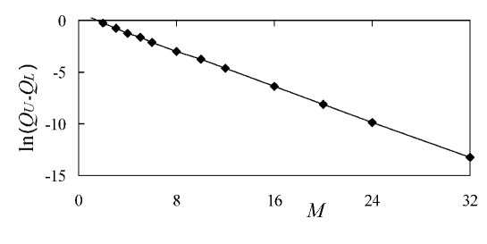
Figure 1: Double knock-out call on a single asset considered in Table 2.

Comparison of our biased estimators with the exact analytical result shows that the biases of $Q_{I}$, $Q_{L}$ and $Q_{U}$ are less than their standard errors for $M\geq 4$, $M\geq 4$ and $M\geq 8$ respectively while the bias of the standard estimator $Q_{S}$ is significantly larger than its standard error even for $M$=1024. The standard errors are less then 1% of the true value. The exact value is always inside the standard confidence intervals of the point estimators $Q_{1}$ and $Q_{0}$. In the case where a double barrier is imposed on the asset the hits of the upper and lower barriers are “physically” distant (the asset can not be close to the upper and lower barriers at the same time). Thus intuitively we expect that the bias $Q_{U}-Q_{L}$ should be exponentially small for large $M$. In Figure 1 we plot $\ln(Q_{U}-Q_{L})$ versus $M$ for the case of the double knock-out call considered in Table 2. The standard error of the plotted estimates is less than the size of the symbols. The observed linear behaviour of the graph indicates that the bias decreases as $Q_{U}-Q_{L}\sim e^{-\alpha/\delta t}$.

4.2 Two asset call with two knock-out barriers

To demonstrate convergence of the estimators for the case where barriers are imposed on different arbitrary correlated assets we consider two asset down-and-out call with the lower barriers $h_{1}$ and $h_{2}$ imposed on the first and second assets respectively. In this case the explicit expressions for the probability bounds (13), (14) used in the biased estimators (15) are

$$\begin{array}[]{l}P_{U}^{(m)}=\mathop{\min}\limits_{i=1,..,d}[1-\xi_{i}^{(m)}(h_{i})],\\ P_{I}^{(m)}=\prod\limits_{i=1}^{d}{[1-\xi_{i}^{(m)}(h_{i})]},\\ P_{L}^{(m)}=\max[1-\sum\limits_{i=1}^{d}{\xi_{i}^{(m)}(h_{i})},0],\\ \end{array}$$ (20)

where $d$ = 2. We designed the problem parameters to equate probabilities of the barrier hits $\xi_{1}^{(m)}(h_{1})=\xi_{2}^{(m)}(h_{2})$ if $\rho=\;1$. In this case $P_{L}^{(m)}=\max[1-2\xi_{1}^{(m)}(h_{1}),0]$, $P_{U}^{(m)}=1-\xi_{1}^{(m)}(h_{1})$ and we expect worst convergence because the events of the barrier hits do not become disjoint at $M\to\infty$. The exact joint distribution $P^{(m)}$ can be found in a closed form using the results in He, Keirstead and Rebholz (1998). It is expressed via infinite series (usually the series are rapidly convergent) and can be used to calculate the unbiased estimator (8). Again, being only interested in the convergence of the biased estimators we do not pursue this calculation.

In Table 3 we show the exact prices and Monte Carlo estimators for various asset correlation values. The exact option price for $\rho=-0.5,\;0.5$ has been found via numerical integration of the two-dimensional density function from He, Keirstead and Rebholz (1998). In the cases $\rho=-1,\;0,\;1$ the option value can be expressed via the barrier options on a single asset and the exact solutions are represented via the standard cumulative Normal function. If the correlation, $\rho$, between the assets is positive (negative) then the minima of the assets over the same time interval are always positively (negatively) dependent. Thus the estimator $Q_{I}$ based on the distribution of the independent extremes is always larger (less) than the unbiased estimator $Q$ if $\rho<0$ ($\rho>0)$. We do not present the results for $Q_{1}\approx(Q_{I}+Q_{L})/2$ (if $\rho<0)$ and $Q_{2}\approx(Q_{I}+Q_{U})/2$ (if $\rho>0)$ but they can be used as a better point estimate for the true price instead of $Q_{0}\approx(Q_{U}+Q_{L})/2$. If $\rho=0$ then the minima are independent and $Q_{I}$ is an unbiased estimator for the true price because $P_{I}^{(m)}$ is a valid joint distribution. If $\rho=1$ then the minima of the assets have a perfect positive dependence and $Q_{U}$ is an unbiased estimator because $P_{U}^{(m)}$ is a valid joint distribution.

The obtained results show that our biased estimators $Q_{U}$, $Q_{I}$ and $Q_{L}$ are rapidly convergent to the true value when compared to the standard estimator $Q_{S}$. Comparison of our results with the exact results shows that the biases of $Q_{I}$, $Q_{L}$ and $Q_{U}$ are less then their standard errors if $M\geq 16$ while the bias of the standard estimator $Q_{S}$ is significantly larger than its standard error even for $M$=1024 (the standard errors are less then 1% of the true value for almost all cases). The only case when the convergence of $Q_{I}$ and $Q_{L}$ is not so rapid is $\rho=1$ (in this case $Q_{U}$ is the unbiased estimator). The standard confidence interval of the point estimator $Q_{0}$ always contains the exact price.

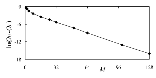
Figure 2: Two asset down-and-out call considered in Table 3 with $\;\rho=-1$.

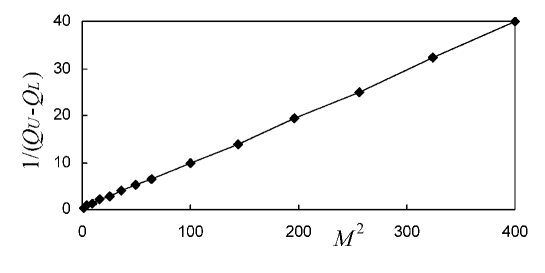
Figure 3: Two asset down-and-out call considered in Table 3 with $\rho=0$.

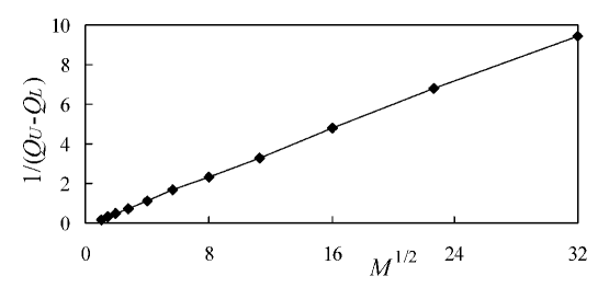
Figure 4: Two asset down-and-out call considered in Table 3 with$\;\rho=1$.

The convergence rate of our biased estimators strongly depends on correlation between the assets. In Figure 2, Figure 3 and Figure 4 we present the graphs indicating the convergence rates for $\rho=-1,\;0,\;1$. The size of the symbols used for the graphs is larger than the standard error of the estimates (we have used more simulations for estimates at large $M)$.

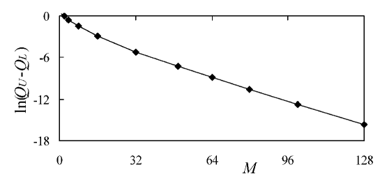
Figure 5: Two asset down-and-out call considered in Table 3 with $\rho=1$ and $S_{1}(0)=95$, $S_{2}(0)=105$.

The linear behaviour of the graphs at large $M$ indicates the following. If $\rho=-1$ then $Q_{U}-Q_{L}\sim e^{-\beta/\delta t}$ for $M>>1$. This is similar to the results for double barrier call in Table 2 and Figure 1, because the assets have a perfect negative dependence and the option is equivalent to a single asset knock-out option with the flat lower and exponentially growing upper barriers . If $\rho=1$ then $Q_{U}-Q_{L}\sim\sqrt{\delta t}$ for $M>>1$. This square root convergence is the worst observed rate. In this case the asset minima have a perfect positive dependence and the estimator $Q_{U}$ is the unbiased estimator of the true option price. That is $Q_{L}$ and $Q_{S}$ converge to the true price at the same rate from below and above respectively. If $\rho=0$ then $Q_{U}-Q_{L}\sim\delta t^{2}$ for $M>>1$. We have observed that the convergence rate smoothly deteriorates from the best exponential decay $\sim\exp(-\beta/\delta t)$ at $\rho=-1$ to a rapid power decay $\delta t^{2}$ at $\rho=0$ and slow square root decreasing $\sim\sqrt{\delta t}$ at $\rho=1$ as the correlation is changed between $-1$ and $1$. Note that we have designed the parameters to get worst convergence at $\rho=1$. If we change the parameters to make the barrier hit probabilities unequal then the extrema should become disjointed as $M\to\infty$ even for $\rho=1$. For example, if we set the asset spots $S_{1}(0)=95$, $S_{2}(0)=105$ and do not change the other parameters then the convergence rate at $\rho=1$ is rapid exponential decay $\sim\exp(-\beta/\delta t)$, see Figure 5, while for $\rho=0$ and $-1$ the rates do not change (that is $\sim\delta t^{2}$ and $\sim\exp(-\beta/\delta t)$ respectively).

4.3 Multi-asset call with multiple barriers

Finally, to show that our biased estimators work well for real multi-dimensional problems we consider, see Table 4, down-and-out call on $d$ underlying assets with the lower barriers imposed on all assets for the cases $d=3$ and $d=10$. The exact (analytical) result is not available for this problem. Explicit expressions for the probability bounds (13), (14) used in the biased estimators (15) are given by (20). As we have chosen positive correlation between all assets the asset minima are positively dependent. Thus $Q_{I}$ is always less than the unbiased estimator $Q$ and we present the results for $Q_{2}\approx(Q_{I}+Q_{U})/2$ which is a better point estimate for the true price than $Q_{0}$. As in the previous examples, all our biased estimators $Q_{U}$, $Q_{I}$ and $Q_{L}$ are rapidly convergent to each other. Their biases become less than the statistical errors for $M\geq 16$ while the bias of the standard estimator $Q_{S}$ is larger than its standard error even for $M=1024$.

5 Conclusions and discussion

In this paper we have developed a conditioning technique, that can be called a Brownian Bridge scheme, for Monte Carlo simulation of a general class of multi-asset options with continuously monitored knock-out barriers imposed for some or all underlying assets. We have derived the general formula (8) for an unbiased estimator of the option based on the joint distribution of the multi-dimensional Brownian Bridge extrema (9). If the distribution is known, for example, one barrier imposed on one of the assets (or two barriers imposed on different or the same assets) per time region, the scheme provides a simple unbiased estimator. The barriers, drifts and volatilities are required to be piecewise constant functions of time. In the case of more than two barriers per time region the distribution is unknown in a closed form for arbitrary dependence between the assets and we derived the upper, $Q_{U}$, and lower, $Q_{L}$, biased option price estimators. The estimators are based on the Fréchet lower, $P_{L}^{(m)}$, and upper, $P_{U}^{(m)}$, bounds (13) for the unknown joint distribution with given univariate margins. We have also used the estimator $Q_{I}$ based on the joint distribution of independent extrema, $P_{I}^{(m)}$. For some simple barrier and dependence structures $Q_{I}$ can provide better upper or lower bounds. While this estimator is usually more accurate, $Q_{L}$ and $Q_{U}$ are often more useful because they can always be used to bind the true option price by the confidence interval. As the time between the sampling dates decreases, the Brownian Bridge extrema become more disjointed and the biased estimators $Q_{L}$, $Q_{I}$, $Q_{U}$ converge to each other and the true value. In the limit, the option price estimator becomes independent of the dependence structure (the so-called copula) of the extrema and depends on their marginal distributions only. In our numerical examples we showed that the bias $Q_{U}-Q_{L}$ is less and convergence is rapid when compared to the bias and convergence of the standard estimator $Q_{S}$ ($Q_{S}-Q\sim\sqrt{\delta t}$ for $M>>1$, where $\delta t=T/M)$. Usually, $Q_{U}-Q_{L}$ is less than the statistical error of the estimates for only a few time steps. In practice, the intermediate dates are introduced due to the interest rate or volatility term-structures and the insertion of the additional sampling dates to eliminate the bias may not be even required. The convergence rate depends on the barrier and correlation structures. We have always observed $Q_{U}-Q_{L}\sim\exp(-\alpha/\delta t)$ for the case of lower and upper barriers imposed on the same asset. For the case of two lower barriers imposed on two assets the best detected convergence rate is exponential decay $\sim\exp(-\beta/\delta t)$ and the worst detected rate is slow square root decreasing $\sim\sqrt{\delta t}$. The worst case was obtained for the unrealistic special set of parameters ($\rho=1$ and identical parameters for both assets) which makes barrier hits always equal each other and $Q_{U}$ to be an unbiased estimator of the true price.

The described Brownian Bridge technique is straightforward to use for the valuation of the knock-in barrier options and barrier options with constant rebates, $R$, paid at maturity. The unbiased estimators in these cases are given by

$$Q=V(S(T))[1-{\rm I}_{\tau>T}\prod\limits_{m=1}^{M}{P^{(m)}}]$$

and

$$Q=V(S(T)){\rm I}_{\tau>T}\prod\limits_{m=1}^{M}{P^{(m)}}+R\cdot[1-{\rm I}_{\tau>T}\prod\limits_{m=1}^{M}{P^{(m)}}]$$

respectively. The upper and lower biased estimators can easily be calculated using $P_{L}^{(m)}$ and $P_{U}^{(m)}$. The technique can easily be applied to efficiently estimate discretely monitored barrier options with a large number of observation dates using the method proposed by Andersen (1996). That is, using our scheme calculate the continuously monitored barrier option price $Q_{c}$ and using the standard Monte Carlo method estimate the option with a low frequency monitored barrier. Then the interpolation formula $Q_{M}\approx Q_{c}+\lambda/\sqrt{M}$, where $Q_{M}$ is a barrier option with $M$ monitored dates, allows for effective estimation of the option with a high frequency monitored barrier.

Finding the upper and lower biased estimators is not straightforward for the case of multi-barrier options with rebates paid at hitting times. This type of problem is also relevant to the valuation of credit derivatives. To calculate the unbiased option price estimator, multiple hitting times should be simulated from their valid joint distribution which is not known even for the case of two barriers. However, the hitting times can easily be simulated from their known univariate marginal distributions, see Anderson (1996). Thus, again we have a problem of the unknown joint distribution with the known univariate margins. Such options can be evaluated in the following way. Calculate one option estimate $Q^{(\ref{eq1})}$ simulating the hitting times marginally with perfect positive dependence. Another estimate $Q^{(\ref{eq2})}$ can be found by simulating the events marginally with perfect negative dependence in the case of two barriers or simulating the events independently if there are more than two barriers. The difference between $Q^{(\ref{eq1})}$ and $Q^{(\ref{eq2})}$ can be used as a weak criterion for the disjointed events to justify their marginal simulations. That is, if the difference is less than the statistical error then the events can be assumed disjointed enough (marginal simulation is justified) and $(Q^{(\ref{eq1})}+Q^{(\ref{eq2})})/2$ can be used as a point estimate for the true price. Otherwise additional sampling dates need to be inserted. Lookback type options with payoff dependent on a few continuous extrema can be evaluated in a similar way. We will consider these problems in further research.

In all our examples we have assumed the lognormal diffusion process (1) to allow for comparison with analytical results. However, the Brownian Bridge scheme discussed here is still applicable for more general diffusion processes. For example, it is applicable if drifts and volatilities are state-dependent. To solve these models approximate discretisation schemes freezing the drifts and volatilities to the left point of each simulation step are used, see for example Kloeden and Platen (1992). Then Brownian Bridge schemes can be used because the requirements of piecewise constant drifts and volatilities are satisfied. This will eliminate the bias due to discrete underestimation of the continuous extrema (bias due to the discretisation scheme will not be removed).

In this paper we have focused on the application of the technique for the valuation of simple knock-out multi-asset options. However, practical use of the technique lies in a broad range of problems. For example, the technique can potentially be used for credit and market risk problems where valuation of a multi-asset payoff with some barrier levels imposed on the underlying assets is very essential.

Acknowledgements

The author thanks Volf Frishling and Frank de Hoog for stimulating discussions and helpful advice.

References

Andersen, L., and Brotherton-Racliffe, R. (1996). Exact Exotics. Risk, 9(10), 85-89.

Andersen, L. (1996). Monte Carlo simulation of Barrier and Lookback Options with continuous or High-Frequency Monitoring of the Underlying Asset. Working paper, General Re Financial Products.

Andersen, L. (1998). Monte Carlo simulation of Options on Joint Minima and Maxima. Working paper, General Re Financial Products.

Beaglehole, D. R., Dybvig, P. H., and Zhou, G. (1997). Going to extremes: Correcting Simulation Bias in Exotic Option Valuation. Financial Analyst Journal, January/February, 62-68.

Borodin, A., and Salminen, P. (1996). Handbook of Brownian Motion-Facts and Formulae. Birkhauser Verlag, Basel.

Boyle, P., Broadie, M., and Glassermann, P. (1997). Monte Carlo Methods for Security Pricing. Journal of Economic Dynamics and Control, 21, 1267-1321.

Broadie, M., Glasserman, P., and Kou, S. (1997). A continuity correction for discrete barrier options. Mathematical Finance, 7, 325-349.

Cox, D., and Miller, H. (1965). The Theory of Stochastic Processes. Chapman and Hall.

Dewynne, J., and Wilmott, P. (1994). Partial to Exotic. Risk, December, 53-57.

He, H., Keirstead, W. P., and Rebholz, J. (1998). Double Lookback. Mathematical Finance, 8(3), 201-228.

Heynen, R., and Kat, H. (1994a). Partial Barrier Options. Journal of Financial Engineering, 3(3/4), 253-274.

Heynen, R., and Kat, H. (1994b). Crossing barriers. Risk, 7(6), 46-51.

Hull, J., and White, A. (1993). Efficient Procedures for Valuing European and American Path-Dependent Options. Journal of Derivatives, Fall, 21-31.

Joe, H. (1997). Multivariate Models and Dependence Concepts. Chapman & Hall.

Kat, H., and Verdonk, L. (1995). Tree Surgery. Risk, February, 53-56.

Karatzas, I., and Shreve, S. (1991). Brownian Motion and Stochastic Calculus. Springer Verlag.

Kloeden, P., and Platen, E. (1992). Numerical Solution of Stochastic Differential Equations. Springer Verlag.

Kunitomo, N., and Ikeda, M. (1992). Pricing Options with Curved Boundaries. Mathematical Finance, 4, 275-298.

Merton, R. (1973). Theory of Rational Pricing. Bell Journal of Economics and Management Science, 4, Spring, 141-183.

Rubinstein, M., and Reiner, E. (1991). Breaking down the barriers. Risk, 4(8), 28-35.

One asset down and out call. The exact value is 8.794.			Two asset down-and-out call. The exact value is 8.256.
$M$	$Q$(std.err.)	$Q_{S}$(std.err.)	$M$	$Q$(std.err.)	$Q_{S}$(std.err.)
1 2 4 16 64 256 1024	8.79(0.02) 8.80(0.02) 8.80(0.02) 8.79(0.02) 8.80(0.02) 8.80(0.02) 8.80(0.02)	10.91(0.02) 10.66(0.02) 10.32(0.02) 9.74(0.02) 9.33(0.02) 9.08(0.02) 8.94(0.02)	1 2 4 16 64 256 1024	8.26(0.02) 8.26(0.02) 8.27(0.02) 8.27(0.02) 8.28(0.02) 8.28(0.02) 8.28(0.02)	14.93(0.03) 13.62(0.03) 12.35(0.03) 10.52(0.02) 9.47(0.02) 8.90(0.02) 8.59(0.02)

Table 1: One asset down and out call: $S_{1}(0)=100$, $K=100$, $h_{1}=90$, $\sigma_{1}=0.3$, $r=0.1$, $T=0.5$, $400\,000$ simulations. Two asset down-and-out call with a single barrier: $S_{1}(0)=S_{2}(0)=100$, $K=100$, $h_{2}=90$, $r=0.1$, $T=1$, $\sigma_{1}=\sigma_{2}=0.3$, $\rho=0.5$, $800\,000$ simulations.

$M$	$Q_{U}$(std.err.)	$Q_{I}$(std.err.)	$Q_{L}$(std.err.)	$Q_{S}$(std.err.)	$Q_{1}$(std.err.)	$Q_{0}$(std.err.)
1 2 4 8 16 64 256 1024	3.01(0.01) 2.21(0.01) 1.84(0.01) 1.79(0.01) 1.78(0.01) 1.78(0.01) 1.78(0.01) 1.78(0.01)	2.41(0.01) 1.89(0.01) 1.79(0.01) 1.79(0.01) 1.78(0.01) 1.78(0.01) 1.78(0.01) 1.78(0.01)	1.11(0.01) 1.72(0.01) 1.78(0.01) 1.79(0.01) 1.78(0.01) 1.78(0.01) 1.78(0.01) 1.78(0.01)	12.23(0.04) 9.60(0.04) 7.41(0.03) 5.73(0.03) 4.50(0.02) 3.06(0.02) 2.40(0.02) 2.08(0.02)	1.76(0.66) 1.80(0.09) 1.79(0.01) 1.79(0.01) 1.78(0.01) 1.78(0.01) 1.78(0.01) 1.78(0.01)	2.06(0.96) 1.97(0.26) 1.81(0.04) 1.79(0.01) 1.78(0.01) 1.78(0.01) 1.78(0.01) 1.78(0.01)

Table 2: Double knock-out call on a single asset. $h_{1}=900$, $H_{1}=1100$, $S(0)=K=1000$, $\sigma_{1}=0.2$, $r=0.1$, $T=0.5$, $400\,000$ simulations. The exact value of the continuously monitored option is 1.793.

$\rho$	$M$	$Q_{U}$(std.err.)	$Q_{I}$(std.err.)	$Q_{L}$(std.err.)	$Q_{S}$(std.err.)	$Q_{0}$(std.err.)	$Q_{c}$
0	1 8 16 32 64 1024	5.02(0.03) 3.78(0.04) 3.70(0.04) 3.66(0.04) 3.65(0.04) 3.64(0.04)	3.65(0.03) 3.66(0.04) 3.66(0.04) 3.65(0.04) 3.65(0.04) 3.64(0.04)	2.27(0.02) 3.62(0.04) 3.65(0.04) 3.65(0.04) 3.65(0.04) 3.64(0.04)	11.76(0.07) 6.84(0.06) 5.92(0.05) 5.27(0.05) 4.81(0.05) 3.93(0.05)	3.64(1.41) 3.70(0.12) 3.67(0.06) 3.65(0.05) 3.65(0.04) 3.64(0.04)	3.649
0.5	1 8 16 32 64 1024	7.78(0.05) 6.71(0.06) 6.61(0.06) 6.57(0.06) 6.55(0.06) 6.54(0.06)	5.84(0.04) 6.48(0.05) 6.53(0.06) 6.54(0.06) 6.54(0.06) 6.54(0.06)	4.22(0.04) 6.41(0.05) 6.51(0.06) 6.53(0.06) 6.54(0.06) 6.54(0.06)	14.97(0.08) 10.28(0.07) 9.27(0.07) 8.52(0.07) 7.98(0.06) 6.93(0.06)	6.00(1.82) 6.56(0.20) 6.56(0.10) 6.55(0.07) 6.55(0.06) 6.54(0.06)	6.527
-0.5	1 8 16 32 64 1024	2.57(0.02) 1.47(0.02) 1.42(0.02) 1.41(0.02) 1.39(0.02) 1.38(0.02)	1.70(0.01) 1.41(0.02) 1.40(0.02) 1.40(0.02) 1.39(0.02) 1.38(0.02)	0.67(0.01) 1.40(0.02) 1.40(0.02) 1.40(0.02) 1.39(0.02) 1.38(0.02)	7.86(0.05) 3.63(0.04) 2.88(0.03) 2.45(0.03) 2.09(0.03) 1.55(0.03)	1.62(0.96) 1.43(0.06) 1.41(0.03) 1.41(0.02) 1.39(0.02) 1.38(0.02)	1.395
1.0	1 8 16 32 64 1024	11.36(0.06) 11.36(0.07) 11.37(0.07) 11.35(0.07) 11.34(0.07) 11.33(0.07)	8.05(0.05) 10.22(0.07) 10.63(0.07) 10.84(0.07) 10.98(0.07) 11.24(0.07)	6.31(0.05) 10.00(0.07) 10.49(0.07) 10.74(0.07) 10.91(0.07) 11.22(0.07)	16.79(0.08) 14.35(0.08) 13.63(0.08) 13.06(0.07) 12.63(0.07) 11.69(0.07)	8.84(2.58) 10.68(0.74) 10.93(0.51) 11.04(0.37) 11.12(0.29) 11.28(0.12)	11.315
-1.0	1 8 16 32 64 1024	0.415(0.002) 0.018(0.001) 0.014(0.001) 0.014(0.001) 0.013(0.001) 0.013(0.001)	0.167(0.001) 0.014(0.001) 0.013(0.001) 0.014(0.001) 0.013(0.001) 0.013(0.001)	0(0) 0.014(0.001) 0.013(0.001) 0.014(0.001) 0.013(0.001) 0.013(0.001)	2.839(0.018) 0.476(0.008) 0.250(0.06) 0.137(0.004) 0.080(0.003) 0.023(0.002)	0.207(0.209) 0.016(0.003) 0.014(0.001) 0.014(0.001) 0.013(0.001) 0.013(0.001)	0.0131

Table 3: Two asset down-and-out call with lower barriers for the first and second assets. $h_{1}=h_{2}=90$, $S_{1}(0)=S_{2}(0)=100$, $K=100$, $\sigma_{1}=\sigma_{2}=0.3$, $r=0.1$, $T=1$, $100\,000$ simulations. $Q_{c}$ is the exact value of the option with continuously monitored barriers.

$d$	$M$	$Q_{U}$(std.err.)	$Q_{I}$(std.err.)	$Q_{L}$(std.err.)	$Q_{S}$(std.err.)	$Q_{2}$(std.err.)	$Q_{0}$(std.err.)
3	1 2 4 8 16 32 64 1024	8.96(0.07) 8.26(0.07) 7.83(0.07) 7.65(0.07) 7.60(0.08) 7.60(0.08) 7.60(0.08) 7.60(0.08)	6.69(0.06) 7.20(0.07) 7.43(0.07) 7.51(0.07) 7.56(0.08) 7.59(0.08) 7.59(0.08) 7.60(0.08)	5.13(0.06) 6.76(0.07) 7.31(0.07) 7.47(0.07) 7.54(0.08) 7.58(0.08) 7.59(0.08) 7.60(0.08)	14.96(0.10) 13.27(0.09) 11.81(0.09) 10.76(0.09) 9.96(0.09) 9.29(0.08) 8.80(0.08) 7.91(0.08)	7.83(1.20) 7.73(0.60) 7.63(0.27) 7.58(0.14) 7.58(0.10) 7.59(0.08) 7.59(0.08) 7.60(0.08)	7.04(1.97) 7.51(0.82) 7.57(0.33) 7.56(0.16) 7.57(0.11) 7.59(0.09) 7.59(0.08) 7.60(0.08)
10	1 2 4 8 16 32 64 1024	4.62(0.05) 3.56(0.05) 2.98(0.05) 2.80(0.05) 2.71(0.05) 2.67(0.05) 2.65(0.05) 2.65(0.05)	1.19(0.02) 1.97(0.03) 2.39(0.04) 2.60(0.05) 2.64(0.05) 2.65(0.05) 2.64(0.05) 2.65(0.05)	0.21(0.01) 1.33(0.03) 2.20(0.04) 2.54(0.05) 2.61(0.05) 2.64(0.05) 2.64(0.05) 2.65(0.05)	10.36(0.09) 7.92(0.08) 6.13(0.07) 5.09(0.07) 4.37(0.06) 3.84(0.06) 3.48(0.06) 2.86(0.05)	2.90(1.75) 2.77(0.84) 2.68(0.34) 2.70(0.15) 2.67(0.08) 2.66(0.06) 2.65(0.05) 2.65(0.05)	2.41(2.23) 2.45(1.16) 2.59(0.44) 2.67(0.18) 2.66(0.10) 2.66(0.07) 2.64(0.06) 2.65(0.05)

Table 4: Knock-out calls on three and ten assets with lower barriers for each of the asset. $S_{i}(0)=100$, $h_{i}=80$, $\rho_{ij}=0.5$ if $i\neq j$, $\sigma_{i}=0.4$ ($i,j=1,...,d)$, $T=1$, $K=100$, $r=0.05$, $100\,000$ simulations.