Interactions between two-dimensional solitons in the diffractive-diffusive Ginzburg-Landau equation with the cubic-quintic nonlinearity

Abstract

We report results of systematic numerical analysis of collisions between two and three stable dissipative solitons in the two-dimensional (2D) complex Ginzburg-Landau equation (CGLE) with the cubic-quintic (CQ) combination of gain and loss terms. The equation may be realized as a model of a laser cavity which includes the spatial diffraction, together with the anomalous group-velocity dispersion (GVD) and spectral filtering acting in the temporal direction. Collisions between solitons are possible due to the Galilean invariance along the spatial axis. Outcomes of the collisions are identified by varying the GVD coefficient, $\beta$, and the collision “velocity” (actually, it is the spatial slope of the soliton’s trajectory). At small velocities, two or three in-phase solitons merge into a single standing one. At larger velocities, both in-phase soliton pairs and pairs of solitons with opposite signs suffer a transition into a delocalized chaotic state. At still larger velocities, all collisions become quasi-elastic. A new outcome is revealed by collisions between slow solitons with opposite signs: they self-trap into persistent wobbling dipoles, which are found in two modifications – horizontal at smaller $\beta$, and vertical if $\beta$ is larger (the horizontal ones resemble “zigzag” bound states of two solitons known in the 1D CGL equation of the CQ type). Collisions between solitons with a finite mismatch between their trajectories are studied too.

I Introduction

Complex Ginzburg-Landau equations (CGLEs) constitute a vast class of models for the pattern-formation dynamics and spatiotemporal chaos in one- and multidimensional nonlinear media combining dissipative and dispersive/diffractive properties CGL . In particular, stable localized pulses (“dissipative solitons” DS ) can be supported by CGLEs that meet the obvious necessary condition of the stability of the zero background. This condition rules out the simplest cubic CGLE, whose one-dimensional (1D) variant admits well-known exact analytical solutions for solitary pulses Lennart . The stability can be achieved in systems of linearly coupled equations, with one featuring linear gain and the other – linear loss coupled . In such a model, exact stable solutions for 1D solitons are available exact . Another possibility is to use the CGLE with the cubic-quintic (CQ) combination of nonlinear terms. For the first time, the CGLE of the CQ type was introduced by Petviashvili and Sergeev PetSer in the 2D form, with the intention to construct stable fully localized 2D states. In 1D, stable dissipative solitons of the CQ CGLE had been later studied in detail Thual , including the analysis of two-soliton bound states bound ; oscill . Then, stable fundamental solitons Deissler ; we ; HS and localized vortices (alias spiral solitons) Bucharest ; HS have been found in 2D and 3D 3D models of the CQ-CGLE type, as well as in the Swift-Hohenberg equation with the CQ nonlinearity SB . Such equations find their most significant physical realization as models of large-area laser cavities, where the CQ combination of the loss and gain is provided by the integration of linear amplifiers and saturable absorbers cavity .

In most above-mentioned works PetSer , HS -SB , localized pulses and vortices were obtained as solutions to isotropic 2D equations. On the other hand, the CGLE which governs the spatiotemporal evolution of light in the large-area laser cavity is anisotropic, as its includes “diffusion” (the spectral filtering) acting only along the temporal variable. The existence of stable fully localized pulse solutions in the latter case suggest a possibility of the experimental creation of “light bullets”, i.e., spatiotemporal optical solitons, in the cavities. In other physical contexts (unrelated to optics), anisotropy of the 2D CGLE was introduced in a different form, through unequal diffusion coefficients in the two perpendicular directions Rabin .

In Refs. we , stable spatiotemporal dissipative solitons were found in the model of the laser-cavity type, based on the following normalized CGLE with the CQ nonlinearity:

$$iU_{Z}+\frac{1}{2}U_{XX}+\frac{1}{2}\left(\beta-i\right)U_{TT}=-\left[iU+\left(1-i\gamma_{1}\right)|U|^{2}U+i\gamma_{2}|U|^{4}U\right].$$ (1)

Here, $Z$ and $X$ are the propagation and transverse coordinates in the cavity, and $T\equiv t-Z/V_{0}$ is, as usual, the reduced time, with $t$ the physical time and $V_{0}$ the group velocity of the carrier wave. Term $U_{XX}$ in Eq. (1) represents the transverse diffraction in the paraxial approximation, the coefficients accounting for the above-mentioned spectral filtering, Kerr nonlinearity, and background linear loss are all scaled to be $1$, while $\beta>0$ corresponds to the group-velocity dispersion (GVD). Usually, a necessary condition for the existence of temporal solitons is $\beta>0$ Agr , which implies the anomalous type of the GVD (in the present model, spatiotemporal solitons also tend to be more stable at $\beta>0$ we ). Further, positive coefficients $\gamma_{1}$ and $\gamma_{2}$ in Eq. (1) account for the cubic gain and quintic loss, respectively, which are characteristic features of CQ models. The third-order GVD was also taken into regard in Refs. we , but this term is not considered here, as it does not essentially affect the results reported below. Because it combines the diffraction along $X$ and effective diffusion along $T$, Eq. (1) is called the diffractive-diffusive CGLE we .

Once 2D solitons are available, an issue of obvious interest is to explore collisions between them, provided that they are mobile, i.e., the equation is Galilean invariant. The 2D CGLE with no diffusion obviously satisfies this condition, allowing free motion of solitons or localized vortices in any direction. This property was used in Ref. HS to study collisions between solitons in the isotropic CQ CGLE, as well as their motion in external potentials. It was concluded that collisions between fundamental solitons result in their quasi-elastic passage through each other (with a resultant increase of the relative velocity), or mutual destruction of the solitons, or their merger into a single 2D pulse. In the same model, collisions between vortices demonstrated a quasi-elastic rebound.

The laser-cavity model based on Eq. (1) features the Galilean invariance along the $X$-direction, which means that a moving solution can be generated from a quiescent one by the application of the Galilean boost corresponding to arbitrary “velocity” $P$ (in fact, $P$ is the tilt in the $\left(X,Z\right)$ plane):

$$U\left(X,T,Z\right)\rightarrow\exp\left[i\left(PX-P^{2}Z/2\right)\right]U\left(X-PZ,T,Z\right).$$ (2)

This possibility suggests to consider collisions of 2D solitons in this model too. In this work, we report results obtained by means of systematic simulations of collisions between two and three solitons in the framework of Eq. (1). In the former case, both head-on collisions and those with a finite offset (aiming distance) between trajectories of the two solitons will be studied. In either case, we consider collisions between in-phase and out-of-phase 2D solitons (the latter means that they have opposite signs).

In Section II, we report the results for two-soliton collisions, and in Section III – for interactions between three solitons. Outcomes of the collisions between two in-phase solitons include the quasi-elastic passage at large velocities, delocalization in the $X$-direction (merger into an expanding quasi-turbulent state) at intermediate velocities, and merger of slowly moving solitons into a single stable pulse. A major difference for collisions between out-of-phase solitons is that, at small velocities, they do not merge into a single pulse; instead, they may form a new localized object – a wobbling dipole, i.e., a robust bound state of two solitons with opposite signs, which feature persistent oscillations relative to each other in the spatial direction. Moreover, two different species of the wobbling dipoles are reported below, horizontal and vertical ones. In the latter case, the out-of-phase solitons, although they collide head-on, shift in opposite perpendicular directions (along the $T$-axis), and eventually form a dipole with a fixed vertical separation between them. Unlike the results for collisions between dissipative solitons in the 2D isotropic CGLE HS , in the present model we have never observed complete destruction (decay) of colliding solitons. For collisions with a finite aiming distance $\Delta T$, we identify a critical value of $\Delta T$ which separates interactions and the straightforward passage. Three-soliton configurations feature either merger into a single pulse, or the transition into a delocalized chaotic state. In terms of the optical cavities, the various outcomes of the collisions offer possibilities for the use in all-optical data-processing schemes.

II Two-soliton collisions

II.1 The numerical procedure

Equation (1) was solved by means of the 2D split-step Fourier method with $256\times 256$ modes and periodic boundary conditions in $X$ and $T$, for the fixed size of the integration domain in both directions, $\left|X,T-10\right|\leq 10$. The stepsize for the advancement in $Z$ was $0.01$. To generate the first stable 2D pulse boosted to velocity (tilt) $P$, cf. Eq. (2), an initial configuration was taken as

$$U_{0}\left(X,T\right)=\exp\left[-\left(X^{2}+T^{2}\right)/4+iPX\right],$$ (3)

see the first panel in Fig. 2 below. The numerical integration of Eq. (1) led to quick self-trapping of the input pulse into a moving (tilted) dissipative soliton, which is an attractor of the model. The profile of the established soliton can be seen in the first panels of Figs. 3 and 5.

Generic results for collisions between the solitons with velocities $\pm P$ can be adequately represented by fixing the cubic gain and quintic loss coefficients to be $\gamma_{1}=2.5$, $\gamma_{2}=0.5$, while varying $P$ and GVD coefficient $\beta$. To generate diagrams presented below in Figs. 1 and 4, which display outcomes of the collisions, we changed $\beta$ and $P$ by small steps, the initial configuration for each simulation being a stable pulse produced by the simulations at the previous step.

II.2 Head-one collisions between in-phase solitons

Outcomes of collisions between two identical stable solitons, set by kicks $\pm P$ on the head-on collision course, are summarized in Fig. 1. Stable solitons exist only for $\beta\geq\beta_{\min}\approx-0.5$, which determines the left-hand edge of the diagram.

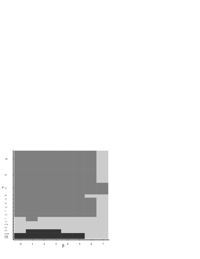
Figure 1: The diagram of outcomes of head-on collisions between identical in-phase solitons, moving at velocities $\pm P$ (the values of $P$ are shown on the logarithmic scale). The black, light gray, and dark gray colors mark parameter regions where the merger, transition to a chaotic delocalized state, and quasi-elastic passage have been observed.

The simplest outcome of the collision is the straightforward quasi-elastic passage of the solitons through each other. We do not illustrate it by a separate picture, as it seems quite obvious; as well as in Refs. we , the solitons keep the mutual symmetry after the quasi-elastic collision, and demonstrate some increase of “velocity” $P$ (recall it is actually defined as the tilt of the soliton’s trajectory in the $\left(X,Z\right)$ plane). Moreover, running the simulations in the domain with periodic boundary conditions, we observed multiple quasi-elastic collisions between solitons. The solitons which emerge unscathed from the first collision survive indefinitely many repeated collisions as well.

With the decrease of the collision velocity, the quasi-elastic passage is changed by the delocalization. This means that two in-phase solitons, interacting attractively, merge into a single pulse, which, however, fails to self-trap into a standing soliton. Instead, it gives rise to a quasi-chaotic (“turbulent”) state, that remains localized in the temporal direction ($T$), but features indefinite expansion along $X$, see a typical example in Fig. 2. This outcome may be explained by the fact the fused state has too much “intrinsic inertia”, imparted by original velocities $\pm P$, which pushes the pulse to expand.

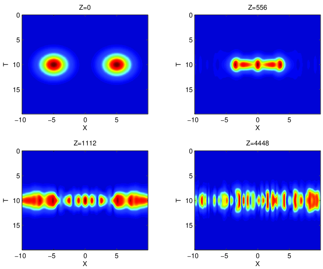
Figure 2: (Color online) A typical example of the transition to delocalization along the $x$ direction, triggered by the merger of colliding in-phase solitons with velocities $P=\pm 0.78$, for $\beta=1$. The evolution of the wave field is illustrated by a set of snapshots of the distribution of $\left|U\left(X,T\right)\right|$. Note that the profiles displayed in the first panel (for $Z=0$) pertain not to the established solitons, but to input (2). Profiles of the established solitons generated from these inputs can be seen below in the first panels of Figs. 3 and 5.

At still smaller values of $P$, the collision also gives rise to merger of the two solitons into a single pulse. However, in that case, the decrease of the above-mentioned “intrinsic inertia” allows the fused pulse to form a stable soliton, see a typical example in Fig. 3.

Figure 3: (Color online) An example of the merger of colliding in-phase solitons into a single stable one, for $P=\pm 0.078$, $\beta=1$.

Before proceeding to the presentation of results obtained for collisions between solitons with opposite signs, it is relevant to mention that we have also considered collisions of solitons with the phase difference of $\pi/2$. In that case (not shown here in detail), the merger of two solitons into a single one is also observed at small velocities, but under more specific conditions. In particular, for $P\leq 0.78$, the merger takes place in the region of $1\leq\beta\leq 3$, which is essentially narrower than the merger region for in-phase solitons, cf. Fig. 1. The reduction of the merger region is quite natural, as the interaction between the solitons is weaker in this case than between in-phase solitons.

II.3 Head-on collisions between solitons with opposite signs

The diagram summarizing outcomes of collision between solitons with opposite signs is displayed in Fig. 4.

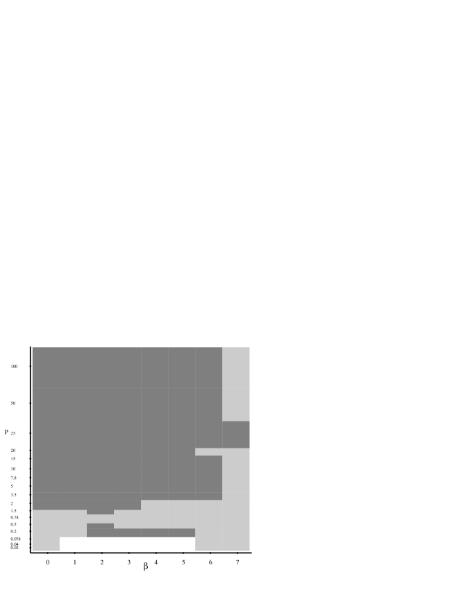
Figure 4: The diagram of head-on collisions between identical solitons with opposite signs. As in Fig. 1, the light and dark gray colors designate regions of the transition to chaotic delocalized states, and quasi-elastic passage, respectively. In the white area, the slowly colliding solitons form horizontal or vertical wobbling dipoles, see the text.

The out-of-phase solitons with large velocities $\pm P$ pass through each other quasi-elastically. Moreover, because the simulations were run with the periodic boundary conditions, we could actually observe multiple collisions, which kept their quasi-elastic character indefinitely long, similar to what was observed in the case of collisions between fast in-phase solitons, as mentioned above. At smaller (intermediate) velocities, collisions between the solitons with opposite signs give rise to the formation of chaotic states indefinitely expanding along $X$, again similar to what was reported above for the case of in-phase solitons (therefore, examples of these outcomes are not displayed here).

A new outcome is produced by collisions of slowly moving out-of-phase solitons. They do not merge into a single pulse, because this is prevented by the mutual repulsion. As seen in the left-hand part of Fig. 5, the solitons come close to each other and then bounce back, but do not separate. Instead, they arrange themselves into a persistent bound state in the form of a “wobbling dipole”. This observation is illustrated by the right-hand side of Fig. 5, which displays trajectories of centers of both solitons in the plane of $\left(X,Z\right)$. Persistent oscillations of the bound solitons lasted as long as the simulations were run. Note that the range of the evolution distance in Fig. 5, $Z=15\cdot 10^{4}$, is extremely large in comparison with the soliton’s diffraction, dispersion, and filtering lengths, which can be estimated as $Z_{\mathrm{diffr}}\sim Z_{\mathrm{disp}}\sim Z_{\mathrm{filt}}\sim 1$ in the present situation, following the usual definitions, $Z_{\mathrm{diffr}}\sim W_{X}^{2}$, $Z_{\mathrm{disp}}\sim W_{T}^{2}/\beta$, $Z_{\mathrm{filt}}\sim W_{T}^{2}$, where $W_{X}$ and $W_{T}$ are the soliton’s widths in the spatial and temporal directions Agr (here, the notation is implied to be as in Eq. (1)). Dependences of the amplitude and frequency of the oscillations on GVD coefficient $\beta$ is not shown here, as the dependence is quite weak.

$\begin{array}[]{cc}\includegraphics[width=225.48424pt]{Fig5.eps}&\includegraphics[width=208.13574pt]{Fig5e.eps}\end{array}$

Figure 5: (Color online) Panels in the left-hand half illustrate the formation of a horizontal “wobbling dipole” as a result of the head-on collision between slowly moving out-of-phase solitons, for $P=\pm 0.078$, $\beta=1$. The panel in the right-hand half shows trajectories of centers of the two solitons, in the same case.

It is relevant to mention that similar stable wobbling bound states of dissipative solitons were reported in simulations of a system of two CQ CGLEs coupled by cubic terms, in the 1D setting, with a group-velocity mismatch between the two equations Brand (in those works, they were called “zigzag” states). On the other hand, in the framework of the single CQ CGLE in 1D, truly stable bound states do not exist, although some of them may be almost stable oscill , with the difference that the phase shift between the two solitons is $\pi/2$ (rather than $\pi$). Thus, the existence of the stable oscillatory dipolar bound states in the single equation is a new feature of the 2D setting.

The formation of the wobbling dipole follows the above scenario in the region of $\beta\leq 3$. At larger values of the GVD coefficient (in particular, at $\beta=4$ and $5$), the repulsive interaction of slowly moving out-of-phase solitons leads to their shift in the transverse direction (to positive and negative values of $T$). Eventually, they form a vertically aligned (“stacked”) wobbling dipole, as illustrated by a set of snapshots in the left-hand side of Fig. 6. The vertical dipole keeps a constant vertical (i.e., temporal) separation between the two solitons stacked in it, which simultaneously perform persistent oscillations in the horizontal direction (along $X$), as seen in the right-hand side of Fig. 6.

$\begin{array}[]{cc}\includegraphics[width=225.48424pt]{Fig6.eps}&\includegraphics[width=208.13574pt]{Fig6e.eps}\end{array}$

Figure 6: (Color online) The same as in Fig. 5, but in the case when the collision of slowly moving solitons with opposite signs ends up with the formation of the vertical “wobbling dipole”, at $\beta=5$.

II.4 Collisions at a finite aiming distance

Collisions between slowly moving in-phase solitons, with a finite offset, $\Delta T$, between their initial trajectories in the vertical direction (alias the aiming distance), also result in the merger into a single quiescent pulse, provided that both $\Delta T$ and velocities are small enough. However, the transition to the delocalization, similar to that shown in Fig. 2, was not observed at finite $\Delta T$. In the same case, collisions between solitons with opposite signs result in a simple dynamical effect, a rebound in the vertical direction. Namely, due to the repulsion between the out-of-phase solitons, the value of $\Delta T$ increases after the collision. These outcome are not shown here, as they are quite obvious.

Varying collision velocities $\pm P$, it is possible to find a critical value of the offset, such that the interaction becomes negligible if $\Delta T$ exceeds the critical offset. For both cases of the in-phase and $\pi$-out-of phase soliton pairs, the critical value is shown, as a function of the velocity, in Fig. 7.

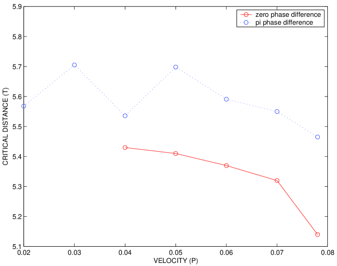
Figure 7: (Color online) The critical value of the offset between initial trajectories of two solitons ($\Delta T$ in the text), in the case of non-head-on collisions. If the offset exceeds the critical value, the solitons effectively cease to interact. This value is shown versus the initial velocities, $\pm P$, separately for in-phase and out-of-phase soliton pairs.

III Three-solitons collisions

Once the character of the two-soliton collisions has been understood, the next natural step is to analyze collisions between three solitons. To this end, we took triplets of identical solitons, with initial velocities $+P,$ $0,$ $-P$. The systematic analysis was restricted to the most interesting case of the collisions between slow solitons, with $P\leq 0.078$.

First, we consider symmetric configurations, with solitons’ signs $\left(+,+,+\right)$ and $\left(+,-,+\right)$. In the former case, the outcome of the collision in the entire region where the simulations were run, $0\leq\beta\leq 7$, is the merger of the triplet of in-phase solitons into a single pulse, see an example in Fig. 8. In the latter case, the triplet of solitons with alternating signs always features the transition to delocalization. A noteworthy peculiarity observed in the case of $\left(+,-,+\right)$ is formation of a transient “wobbling tri-pole” configuration, that qualitatively resembles horizontal wobbling dipoles generated by collisions of two solitons with opposite signs, see Fig. 5. Nevertheless, the “tri-pole” eventually collapses, initiating the transition into an expanding chaotic delocalized state.

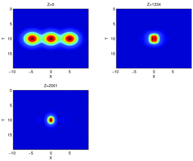
Figure 8: (Color online) The merger of three in-phase solitons into a single one, at $\beta=1$. Initially, edge solitons move at velocities $\pm 0.078$.

The collision-induced transformation of the asymmetric triplet formed by three identical solitons, of type $\left(+,+,-\right)$, was investigated too. As shown in Fig. 9, in this case, two in-phase solitons merge into a single one, at the first stage of the evolution (the middle panel in Fig. 9). Eventually, the intermediate pair of the two pulses also demonstrates a transformation into a single residual soliton.

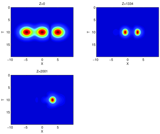
Figure 9: (Color online) The same as in Fig. 8, but starting with the asymmetric triplet of solitons, configured as $\left(+,+,-\right)$.

IV Conclusion

We have undertaken the systematic analysis of collisions between two and three solitons in the 2D CGLE (complex Ginzburg-Landau equation) with the CQ (cubic-quintic) nonlinearity, which may be considered as a model of large-area laser cavities, with the solitons representing spatiotemporal “light bullets” in it. This model, which includes the diffraction in the spatial direction ($X$) and both the GVD (group-velocity dispersion) and spectral filtering in the temporal direction, is Galilean invariant in the former direction, which makes it possible to create moving solitons and collide them. Outcomes of the collisions were systematically studied by varying the GVD coefficient, $\beta$, collision velocity, and relative sign of the solitons.

In the case of collisions between two in-phase solitons, three outcomes have been identified: the merger into a single standing soliton, transition into an expanding delocalized chaotic state, and quasi-elastic passage. Collisions between solitons with opposite signs at small velocities lead, instead of the merger, to a novel outcome – the formation of robust “wobbling dipoles”, which exist in two modifications: horizontal at smaller values of $\beta$, and vertical ones at larger $\beta$. In the 1D setting, oscillatory bound states of dissipative solitons of the “zigzag” type were found in a system of two nonlinearly coupled CQ CGLEs Brand , but truly stable bound states in the single equation of this type do not exist. The stable “wobbling dipoles”, especially their “vertical” variety (the one shown in Fig. 6), is a feature specific to the 2D model. We have also investigated two-soliton collisions with a finite aiming distance, and identified its critical size beyond which the solitons cease to interact.

Collisions between three slowly moving in-phase solitons lead to their merger into a single one, while three solitons with alternating signs form a transient “tri-pole” state, which eventually collapses into a delocalized chaotic state. Three solitons which form an asymmetric configuration, of type $\left(+,+,-\right)$, also merge into a single pulse.

References

- (1) I. S. Aranson, L. Kramer, Rev. Mod. Phys. 74 (2002) 99 (2002); B. A. Malomed, in: Encyclopedia of Nonlinear Science, p. 157 (ed. by A. Scott; New York, Routledge, 2005). N. N. Rosanov, Spatial Hysteresis and Optical Patterns (Springer, Berlin, 2002).
- (2) N. Akhmediev and A. Ankiewicz (Eds.), Dissipative Solitons, Lect. Notes Phys. 661, Springer, Berlin, 2005;
- (3) L. M. Hocking, K. Stewartson, Proc. R. Soc. London Ser. A 326 (1972) 289; N. R. Pereira, L. Stenflo, Phys. Fluids 20 (1977) 1733.
- (4) B. A. Malomed, H. G. Winful, Phys. Rev. E 53 (1996) 5365; J. Atai and B. A. Malomed, Phys. Rev. E 54 (1996) 4371 (1996); B. A. Malomed, Chaos 17 (2007) 037117.
- (5) J. Atai and B. A. Malomed, Phys. Lett. A 246 (1998) 412.
- (6) A. M. Sergeev and V. I. Petviashvili, Dokl. AN SSSR 276 (1984) 1380 [Sov. Phys. Doklady 29 (1984) 493].
- (7) B. A. Malomed, Physica D 29 (1987) 155 (see Appendix of this paper); O. Thual, S. Fauve, J. Phys. (Paris) 49 (1988) 1829; W. van Saarloos, P. C. Hohenberg, Phys. Rev. Lett. 64 (1990) 749; V. Hakim, P. Jakobsen, and Y. Pomeau, Europhys. Lett. 11 (1990) 19; B. A. Malomed, A.A. Nepomnyashchy, Phys. Rev. A 42 (1990) 6009; P. Marcq, H. Chaté, R. Conte, Physica D 73 (1994) 305; N. Akhmediev, V. V. Afanasjev, Phys. Rev. Lett. 75 (1995) 2320.
- (8) O. Thual, S. Fauve, J. Phys. (Paris) 49 (1988) 1829; R. J. Deissler, H. R. Brand, Phys. Rev. A 44 (1991) R3411.
- (9) H. Sakaguchi, B. A. Malomed, Physica D 159 (2001) 91; 167 (2002) 123.
- (10) H. Sakaguchi, Physica D 210 (2005) 138.
- (11) B. A. Malomed, Phys. Rev. A 44 (1991) 6954; B. A. Malomed, Phys. Rev. E 47 (1993) 2874.
- (12) V. V. Afanasjev, N. Akhmediev, Phys. Rev. E 53 (1996) 6471; V. V. Afanasjev, B. A. Malomed, P. L. Chu, Phys. Rev. E 56 (1997) 6020.
- (13) D. Y. Tang, W. S. Man, H. Y. Tam, P. D. Drummond, Phys. Rev. A 64 (2001) 033814.
- (14) L.-C. Crasovan, B. A. Malomed, D. Mihalache, Phys. Rev. E 63 (2001) 016605.
- (15) V. Skarka, N. B. Aleksić, Phys. Rev. Lett. 96 (2006) 013903; D. Mihalache, D. Mazilu, F. Lederer, H. Leblond, B. A. Malomed, Phys. Rev. A 75 (2007) 033811; 76 (2007) 045803; 77 (2008) 033817; N. B. Aleksić, V. Skarka, D. V. Timotijević, D. Gauthier, Phys. Rev. A 75 (2007) 061802.
- (16) H. Sakaguchi, H. R. Brand, Physica D 117 (1998) 95.
- (17) H. R. Brand, R. J. Deissler, Physica A 204 (1994) 87; Phys. Rev. E 51 (1995) R852; W. J. Firth, A. J. Scroggie, Phys. Rev. Lett. 76 (1996) 1623; M. Brambilla, L. A. Lugiato, F. Prati, L. Spinelli, W. J. Firth, Phys. Rev. Lett. 79 (1997) 2042; D. Michaelis, U. Peschel, F. Lederer, Opt. Lett. 23 (1998) 337; G. L. Oppo, A. J. Scroggie, W. J. Firth, J. Opt. B Quant. Semicl. Opt. 1 (1999) 133; M. Tlidi, P. Mandel, Phys. Rev. A 59 (1999) R2575; R. Vilaseca, M. C. Torrent, J. Garcia-Ojalvo, M. Brambilla, M. San Miguel, Phys. Rev. Lett. 87 (2001) 083902. D. V. Skryabin, A. G. Vladimirov, Phys. Rev. Lett. 89 (2002) 044101; E. A. Ultanir, G. I. Stegeman, D. Michaelis, C. H. Lange, F. Lederer, Phys. Rev. Lett. 90 (2003) 253903. N. N. Rosanov, S. V. Fedorov, A. N. Shatsev, J. Exp. Theor. Phys. 102 (2006) 547.
- (18) R. Brown, A. L. Fabrikant and M. I. Rabinovich, Phys. Rev. E 47 (1993) 4141; H. Sakaguchi, Progr. Theor. Phys. 99 (1998) 33; R. B. Hoyle, Phys. Rev. E 58 (1998) 7315.
- (19) G. P. Agrawal. Nonlinear Fiber Optics (Academic Press: San Diego, 1995).
- (20) O. Descalzi, J. Cisternas, H. R. Brand, Phys. Rev. E 74, 065201(R) (2006); O. Descalzi, J. Cisternas, P. Gutiérrez, and H. R. Brand, Eur. Phys. J. Special Topics 146 (2007) 63.