The viscous overstability, nonlinear wavetrains, and finescale structure in dense planetary rings

Abstract

This paper addresses the fine-scale axisymmetric structure exhibited in Saturn’s A and B-rings. We aim to explain both the periodic microstructure on 150–220m, revealed by the Cassini UVIS and RSS instruments, and the irregular variations in brightness on 1–10km, reported by the Cassini ISS. We propose that the former structures correspond to the peaks and troughs of the nonlinear wavetrains that form naturally in a viscously overstable disk. The latter variations on longer scales may correspond to modulations and defects in the wavetrains’ amplitudes and wavelength. We explore these ideas using a simple hydrodynamical model which captures the correct qualitative behaviour of a disk of inelastically colliding particles, while also permitting us to make progress with analytic and semi-analytic techniques. Specifically, we calculate a family of travelling nonlinear density waves and determine their stability properties. Detailed numerical simulations that confirm our basic results will appear in a following paper.

,

1 Introduction

Saturn’s A and B-rings sport an abundance of irregular radial structure which, though aesthetically pleasing, presents something of a puzzle to the theoretician. The instruments aboard the Cassini space probe show that these patterns manifest on a vast range of length-scales and can take quite different forms. For instance, there exist quasi-periodic microstructure on scales of 0.1 km (Colwell et al. 2007; Thomson et al. 2007), discontinuous and irregular striations on the 1-10 km intermediate scale, and much broader 100 km undulations (Porco et al. 2005). In addition to the difficulties involved in tackling these three orders of magnitude, there are the formidable modelling questions posed by a cold disk of densely-packed, inelastic, and infrequently colliding particles (Stewart et al. 1984, Araki and Tremaine 1986, Salo 1991, Hämeen-Antilla and Salo 1993, Schmidt et al. 2001, Latter and Ogilvie 2008). This paper will focus on only a subset of these phenomena, the smaller-scale variations, and will not linger especially on the modelling issues. Specifically, it investigates how the quasi-periodic microstructure relates to the viscous overstability, on one hand, and to structure formation on the intermediate scales, on the other. The variations on the much longer 100km scale are not examined, and we suspect that they have their origin in a different mechanism entirely, perhaps ballistic transport (Durisen 1995).

Our starting point is the viscous overstability, which is now regarded as a key player in the short scale radial dynamics of Saturn’s rings (Schmit and Tscharnuter 1995, Schmidt et al. 2001, Spahn and Schmidt 2006, Latter and Ogilvie 2008). The viscous overstability is an axisymmetric oscillatory instability that afflicts the homogeneous state of Keplerian shear. Growing modes rely on the alliance of the fluid disk’s inertial-acoustic oscillations with the disk’s stress oscillations: variations in the stress extract energy from the Keplerian shear and inject it into the inertial-acoustic wave; but the increased motion this induces magnifies the stress oscillation itself which can extract even more energy, and so the process runs away. The feedback loop requires (a) the stress to efficiently remove energy from the Keplerian flow and (b) the two oscillations to communicate effectively, in particular for them to be in phase. The first condition is tied to the stress’s sensitivity to surface density. The second condition is often violated in dilute rings and turbulent disks, where the stress can lag behind the epicycles and the overstability fails to work (Ogilvie 2001, Latter and Ogilvie 2006a).

The instability’s linear theory has been well established by a variety of theoretical approaches: hydrodynamics (Schmit and Tscharnuter 1995, Schmidt et al. 2001), $N$-body simulations (Salo 2001, Salo et al. 2001), and kinetics (Latter and Ogilvie 2006a, 2008). However, its nonlinear theory has received surprisingly little attention. Two hydrodynamical studies exist, a large-scale nonlinear simulation of a ring annulus in 1D (Schmit and Tscharnuter 1999) and a weakly nonlinear analysis (Schmidt and Salo 2003). The simulations show that the nonlinear evolution of an overstable disk is characterised by significant disorder. In contrast, the latter study suggests that an overstable ring may exhibit simple coherent structures which take the form of travelling waves. Because Schmit and Tscharnuter impose reflecting boundary conditions, and hence break translational symmetry, such coherent structures may have been difficult to observe in their simulations. Certainly, more simulations need to be undertaken and the influence of the boundary conditions better understood. Concurrently, a fully nonlinear theory extending the work of Schmidt and Salo is required to fully establish the existence of the nonlinear solutions. The former project we present elsewhere, the latter we present here.

First, we demonstrate that steady nonlinear travelling wavetrains are exact solutions to the governing nonlinear equations of a viscously overstable disk, and second, that these solutions are the loci of a rich secondary set of dynamics which generate irregular variations in the waves’ amplitude and wavenumber. We propose that viscously overstable regions in the A and B-rings support a bed of travelling wavetrain solutions and these structures correspond to the quasi-periodic variations registered by Cassini’s UVIS and RSS instruments (the radial ‘microstructure’). Modulations and defects in the amplitudes and wavelengths of these wavetrains may yield different optical properties which can be traced by the Cassini cameras. Consequently, we hypothesise that these larger-scale variations are associated with the intermediate 1-10 km structures observed (Porco et al. 2005). Our hypotheses are investigated with a one-dimensional, isothermal fluid model endowed with a Navier-Stokes stress. Though simplistic, it should predict qualitatively correct behaviour, while permitting the problem to be attacked analytically or semi-analytically. Importantly, self-gravity is omitted throughout, but we investigate its role in a following paper. This is mainly for readability as the nonself-gravitating dynamics is sufficiently complex on its own.

A study of nonlinear waves connects naturally to the extensive field of wave propagation in thin astrophysical disks (Kato 2000), and in particular to the launching of spiral density waves (Goldreich and Tremaine 1978a, 1979, 1980, Borderies et al. 1983, 1986, Shu et al. 1985a, 1985b). In the latter studies the emphasis has been on the launching of spiral waves by an external potential, as might issue from a moon, and the damping of such waves by a viscous stress. But the viscous stress can be an engine of growth also, as in the development of global eccentric modes and narrow ringlets (Borderies et al. 1985, Papaloizou and Lin 1988, Lyubarskij et al. 1994, Longaretti and Rappaport 1995, Ogilvie 2001) and the axisymmetric viscous overstability itself (Kato 1978, Schmit and Tscharnuter 1995). In this paper it will be shown that the viscous forces in a planetary ring can balance energy dissipation and injection and thus sustain steady wave structures.

A study of nonlinear wavetrains also connects to the perhaps more massive field of nonlinear waves in general media and 1D reaction–diffusion systems especially, the model equation of which is the complex Ginzburg-Landau equation (Aranson and Kramer 2002). The dynamics of the complex Ginzburg-Landau equation is remarkably rich and may provide a template for the study of viscous overstability in Saturn’s rings. As in a fluid disk, the equation admits a trivial homogeneous solution that is susceptible to an oscillatory linear instability via a Hopf bifurcation (the analogue of the viscous overstability); it also supports both stable and unstable steady nonlinear wavetrains. Variations upon the wavetrains exhibit a wide variety of behaviours ranging from smooth modulations to abrupt jumps in wavenumber and amplitude (sources and shocks), as well as small-scale chaotic fluctuations (Bernoff 1988, Shraiman et al. 1992, Chaté 1994, Aranson and Kramer 2002). In particular, the sources and shocks can partition the radial domain into a one-dimensional cellular structure, in which each ‘cell’ is characterised by a different wavetrain (Chaté 1993, Popp et al. 1994, Ipsen and Hecke 2001). The latter behaviour seems especially pertinent to ring structure on intermediate scales, which Cassini’s cameras show as a pattern of irregularly spaced, disjunct bands (Porco et al. 2005).

A summary of the paper is as follows. First, space will be lent to a discussion of the validity of the simple hydrodynamic model that we employ, the parameters it introduces, and the values these should take. In Section 3, which comes next, a brief summary of the linear stability of the homogeneous state of Keplerian shear will be presented. Though these results have appeared a number of times elsewhere (Schmit and Tscharnuter 1995, Schmidt et al. 2001), we include them for completeness. Section 4 will demonstrate the existence and investigate the properties of axisymmetric, steady, nonlinear, travelling wavetrains in a viscously overstable disk. The nonlinear wave profiles are calculated numerically via the solution of a nonlinear eigenvalue problem and analytically in the limit of long wavelength. We find that an overstable disk supports a one-parameter family of wavetrain solutions, the members of which can be parametrised by their wavenumber $\lambda$. In Section 5 we establish the linear stability of the wavetrains and find that above a critical wavelength $\lambda_{\text{st}}$ the wavetrains are linearly stable. For model parameter values, associated with optical depths of 1–1.5, the critical wavelength is approximately $50H$, where $H$ is the scale height of the disk. The critical wavelength appears consistent with Cassini observations of periodic microstructure. Lastly, in Section 6, we discuss more fully the general nonlinear dynamics of an overstable disk. A rough argument is sketched explaining the upward cascade to longer scales observed in the simulations of Schmit and Tscharnuter (1999) and we suggest that, irrespective of self-gravity, this ‘inverse cascade’ should halt (or at least change qualitatively) once most power reaches a lengthscale near $\lambda_{\text{st}}$. A discussion follows which addresses what this saturated state may look like. Modulations and defects in the wavetrains’ wavenumber and amplitude are touched on, and a multiple-scales analysis presented in which we show that sources and shocks in the wavetrains’ phase may develop. Finally we discuss the relevance of the complex Ginzburg-Landau equation. Section 7 presents our conclusions, in which we summarise the paper, and point out the issues which remain unresolved and necessary future work.

2 The model

In order to bring out the important features of the ring’s nonlinear evolution we employ a simple hydrodynamical model that captures the correct qualitative behaviour while not burdening the analysis or obscuring its interpretation with mathematical complexity. The ring is assumed to be a vertically-averaged, non-self-gravitating, isothermal, ideal gas possessing a Newtonian viscous stress. In addition, the shearing and bulk viscosities depend on surface density as power laws, in accordance with Schmit and Tscharnuter (1995, 1999) and Schmidt et al. (2001). We also work with the shearing sheet approximation, which is a Cartesian representation of a ‘patch’ of disk orbiting the central planet with frequency $\Omega$, and in which $x$ and $y$ denote the radial and azimuthal dimensions respectively (see Goldreich and Lynden-Bell 1965).

The governing equations are

$$\partial_{t}\sigma+\partial_{i}(\sigma u_{i}) =0,$$ (1)

$$\sigma(\partial_{t}u_{i}+u_{j}\partial_{j}u_{i}+2\Omega\epsilon_{izj}u_{j}) =-\sigma\partial_{i}\Phi_{T}-\partial_{i}P+\partial_{j}\Pi_{ij},$$ (2)

where $\sigma$, $P$, and $\Pi_{ij}$ are the vertically integrated density, pressure, and viscous stress, and $u_{i}$ is the planar fluid velocity. The tidal potential is $\Phi_{T}=-3\Omega^{2}x^{2}/2$.

The pressure comes from the ideal gas equation of state

$$P=v_{s}^{2}\sigma,$$ (3)

where $v_{s}$ is the isothermal sound speed. The viscous stress is given by

$$\Pi_{ij}=\nu\sigma(\partial_{i}u_{j}+\partial_{j}u_{i})+(\nu_{b}-{\textstyle\frac{2}{3}}\nu)\sigma(\partial_{k}u_{k})\delta_{ij}.$$ (4)

The kinematic shear and bulk viscosities are parametrised as

$$\nu=\frac{v_{s}^{2}}{\Omega}\,\alpha\left(\frac{\sigma}{\sigma_{*}}\right)^{\beta},\qquad\nu_{b}=\frac{v_{s}^{2}}{\Omega}\,\alpha_{b}\left(\frac{\sigma}{\sigma_{*}}\right)^{\beta},$$ (5)

where $\alpha$, $\alpha_{b}$, and $\beta$ are dimensionless parameters, and $\sigma_{*}$ is the surface density of the homogeneous state of Keplerian shear.

Throughout the paper we employ dimensions so that

$$\Omega=1,\quad v_{s}=1,\quad\sigma_{*}=1.$$

One unit of time is therefore $(2\pi)^{-1}$ times an orbital period and the unit of length is $H\equiv v_{s}/\Omega$, the scale height of the disk. The full set of governing parameters is now $\alpha$, $\alpha_{b}$, and $\beta$.

2.1 Assumptions

Of course, much can be said about each of the model assumptions. We shall say but a little. First, the adoption of vertical averaging limits us to radial scales much longer than the disk scale height, $H$. The shearing sheet on the other hand limits us to scales much shorter than the disk radius. Neither constraint is much of a problem because the lengthscales of the phenomena we examine sit well within this enormous range. More of an issue is the neglect of the vertical motions. For instance, the viscous overstability is usually accompanied by vertical ‘breathing’ or ‘splashing’ and may be significant when combined with nonisothermal behaviour. We, however, leave this issue open for the time being.

A real planetary ring is not generally isothermal. Due to the relative infrequency of collisions, the thermal time-scale is of the same order as the dynamical time-scale, as kinetic theories and $N$-body simulations show (Goldreich and Tremaine 1978b, Stewart et al. 1984, Brahic 1977). That said, when collisions are a little more frequent — as in a dense ring which may support some tens of collisions per orbit — the isothermal model affords an acceptable approximation (Salo et al. 2001, Latter and Ogilvie 2008).

A dense ring is not an ideal gas, and is probably better suited to a polytropic equation of state which can better capture the effects of close packing and nonlocal pressure (Schmidt et al. 2001, Schmidt and Salo 2003, Latter and Ogilvie 2008). We persist, however, with the simpler model in the belief that the errors introduced do not alter the qualitative behaviour.

Finally, it should be acknowledged that the viscous stress of a planetary ring behaves in a way not always captured by a simple Navier-Stokes stress. For instance, in a dilute ring, effects associated with nonlocality in time (‘memory effects’) are important because the translational stress relaxes on a time-scale comparable to the dynamical time-scale (Latter and Ogilvie 2006a). In contrast, a dense ring possesses a stress dominated by the collisional component, and, though local in time, will be a nonlinear function of the rate of strain (Latter and Ogilvie 2008). The Navier-Stokes model, however, offers a reasonable approximation of the dense system, particularly as we may ‘tweak’ the parameter $\beta$ in order to roughly ‘compensate’ for the linearisation in strain.

Self-gravity is excluded in this paper and will be examined separately in a subsequent article. It undoubtedly plays a role in both the axisymmetric and nonaxisymmetric dynamics of an overstable disk but the effects are complicated and deserve a special treatment. In addition, $N$-body simulations show that nonaxisymmetric self-gravity wakes hinder the development of the linear modes (Schmidt et al. 2001), and it is most probable that they impact on the nonlinear dynamics as well. This is an important issue but one that can only be resolved satisfactorily by three-dimensional simulations.

2.2 Parameters

Aside from these theoretical issues, we are encouraged to use the isothermal hydrodynamic model because it predicts qualitatively correct behaviour when compared with $N$-body simulations. The linear growth rates of the overstable modes are adequately approximated (Schmidt et al. 2001) as is the weakly nonlinear evolution of their amplitudes (Schmidt and Salo 2003). For these reasons the hydrodynamic parameter values we use will be set equal to those computed in these studies, in particular, from Salo et al.’s (2001) $N$-body simulations, which treated particles of radius $100$ cm, undergoing collisions according to the Bridges et al. (1984) piecewise power law at a radius of $100,000$ km. Full self-gravity was not included in the simulations, but its compression of the disk thickness was mimicked by increasing the vertical epicyclic frequency of the particles $\Omega_{z}$ (an idea pioneered by Wisdom and Tremaine 1988). In Table 1 we reproduce some of the data of these runs for different optical depth $\tau$ and with a vertical frequency enhancement of $\Omega_{z}/\Omega=3.6$.

These values will serve us only as a guide. The viscous parameters are closely tied to the kinetic parameters of a particular simulation (such as particle size, elasticity law) but their complete functional dependence is far from understood. On the other hand, the kinetic parameters of a real particulate ring are not yet fully constrained. Thus we let $\alpha$, $\alpha_{b}$ and especially $\beta$ take a variety of values. The $\beta$ parameter is the quantity most sensitive to the background optical depth, as we can see from Table 1, and also to self-gravity. With respect to the last point, Schmidt and Salo (2003) have published another set of parameter values from a simulation in which $\Omega_{z}/\Omega=2$, not 3.6, and they find that $\beta$ takes significantly smaller values in this case. On the other hand, the simplifying assumption of a Newtonian stress may require us to vary $\beta$; and indeed, Schmidt and Salo (2003) inflate $\beta$ by up to $13\%$ in order to obtain agreement in their weakly nonlinear analysis. Finally, in a real disk, the existence of gravitational wakes (screened out by the $N$-body simulations we mention) will militate against the development of the overstable modes, meaning that $\beta$ may take a smaller ‘effective’ value. The actual situation, of course, is probably more complicated, not least by the additional effects of nonlocal ‘gravitational viscosity’ (Daisaka et al. 2001).

$\tau$	$\alpha$	$\alpha_{b}$	$\beta$	$v_{s}/\Omega$ (m)
0.5	0.348	1.08	0.67	2.47
1.0	0.357	0.764	1.15	3.29
1.5	0.342	0.681	1.19	4.42
2.0	0.322	0.683	1.55	5.45

Table 1: Nondimensionalised hydrodynamical parameters at different optical depths $\tau$ derived from $N$-body simulations for a disk of $100$ cm radius particles, at a radius of $100,000$ km, undergoing collisions according to the Bridges et al. (1984) elasticity law, with vertical frequency enhancement of $\Omega_{z}/\Omega=3.6$ (Schmidt et al. 2001, Salo et al. 2001).

3 Linear stability of the homogeneous steady state

This section presents a summary of the stability analysis of the homogeneous steady state of Keplerian shear. Though it has been thoroughly examined with various continuum models ( Lin and Bodenheimer 1981, Ward 1981, Stewart et al. 1984, Schmit and Tscharnuter 1995, Spahn et al. 2000, Schmidt et al. 2001, Latter and Ogilvie 2006a, 2008) we repeat the analysis for completeness and to connect it to our nonlinear work in Sections 3 and 4.

Symbol	Definition
$\tau$	Normal geometric optical depth
$\sigma$	Surface density
$\mathbf{u}$, $\mathbf{u}^{\prime}$	Total and perturbation velocities
$\Phi_{T}$	Tidal potential
$P$	Pressure
$\mathbf{\Pi}$	Viscous stress
$f$, $g$	Dimensionless $xx$ and $xy$ component of the pressure tensor
$\nu$, $\nu_{b}$	Shearing and bulk kinematic viscosities
$\alpha$, $\alpha_{b}$	Shearing and bulk ‘alpha’ parameters
$\beta$	Exponent of density dependence of the kinematic viscosities
$v_{s}$	Sound speed
$\Omega$	Orbital frequency
$H=v_{s}/\Omega$	Disk scale height
$k$, $s$	Wavenumber and growth rate of a linear disturbance
$\mu$, $\omega$	Wavenumber and frequency of a nonlinear wavetrain
$c_{p}=\omega/\mu$	Phase speed of a nonlinear wavetrain
$c_{g}=d\omega/d\mu$	Group speed of a nonlinear wavetrain
$\theta=\mu x-\omega t$	Phase variable of a nonlinear wavetrain
$\lambda=2\pi/\mu$	Wavelength of a nonlinear wavetrain
$\lambda_{\text{st}}$	Critical wavelength above which nonlinear wavetrains are linearly stable
$\mathbf{Z}=(\sigma,u_{x}^{\prime},u_{y}^{\prime})$	Solution vector
$u=c_{p}-u_{x}^{\prime}$, $v=u_{y}^{\prime}$	Dimensionless velocity perturbation variables
$q$, $\vartheta(x,t)$	Amplitude and phase variables for asymptotic long wavelength wavetrains
$\delta$	Small ordering parameter
$X=\delta(x-c_{g}t)$, $T=\delta^{2}t$	Long spatial and temporal variables
$\Theta(X,T)$, $K=\Theta_{X}$	Slowly varying phase and wavenumber of a nonlinear wavetrain
$c_{\text{sh}}$	Speed of a travelling shockfront

Table 2: Table of parameters, variables, and symbols

The equations (1) and (2) admit the following equilibrium: $\sigma=1$ and $u_{y}=-(3/2)\,x$, $u_{x}=0$. We introduce a small perturbation so that $\sigma=1+\sigma^{\prime}$ and $\mathbf{u}=-(3/2)\,x\,\mathbf{e}_{y}+\mathbf{u}^{\prime}$. Their linearised equations read

$$\partial_{t}\sigma^{\prime}+\partial_{x}u_{x}^{\prime}=0,$$ (6)

$$\partial_{t}u_{x}^{\prime}-2u_{y}^{\prime}=-\partial_{x}f^{\prime},$$ (7)

$$\partial_{t}u_{y}^{\prime}+\tfrac{1}{2}u_{x}^{\prime}=-\partial_{x}h^{\prime},$$ (8)

with

$$f^{\prime}=\sigma^{\prime}-(\alpha_{b}+\tfrac{4}{3}\alpha)\partial_{x}u_{x}^{\prime},\qquad h^{\prime}=\frac{3}{2}\alpha(1+\beta)\sigma^{\prime}-\alpha\,\partial_{x}u_{y}^{\prime}.$$ (9)

(For a full list of symbols see Table 2.) The first term in the expression for $h^{\prime}$ is the key to the disk’s stability. It couples the variations in the viscous stress with the background shear and thus allows energy to be drawn from the shear and directed into the perturbation. We now represent the perturbation as a Fourier mode $\propto e^{ikx+st}$ where $k$ is the (real) wavenumber and $s$ is the (complex) growth rate. The ansatz is substituted into Eqs (6)-(9) from which one may derive the following dispersion relation,

$$s^{3}+k^{2}(\tfrac{7}{3}\alpha+\alpha_{b})\,s^{2}+\left[1+k^{2}+k^{4}\alpha(\tfrac{4}{3}\alpha+\alpha_{b})\right]s$$

$$\hskip 162.18062pt+\alpha\,k^{2}\left[3(1+\beta)+k^{2}\right]=0.$$ (10)

In the long wavelength limit, $0<k\ll 1$, two instabilities may be distinguished: the viscous instability and the viscous overstability. The former possesses the growth rate

$$s=-3\alpha(1+\beta)\,k^{2}\,\,+\,\,\mathcal{O}(k^{4}),$$

and is unstable if $\beta<-1$. The instability will be extinguished on short wavelengths and the critical $k$ upon which marginal stability resides can be computed from $|k|=\sqrt{-3(1+\beta)}$. Wavelengths shorter than this value are viscously stable. Table 1 states that a dense particulate ring possesses a positive $\beta$ for all $\tau$, and so the viscous mode will probably decay in real dense planetary rings.

The viscous overstability, on the other hand, possesses growth rates

$$s=\pm i\,\left[1+\tfrac{1}{2}k^{2}\right]+\tfrac{1}{2}\left[3\alpha(1+\beta)-(\tfrac{7}{3}\alpha+\alpha_{b})\right]k^{2}\,\,+\,\,\mathcal{O}(|k|^{3}),$$ (11)

and is hence oscillatory, corresponding to either standing waves or right or left-going travelling waves. In the long wavelength regime, overstability emerges if the following criterion is satisfied:

$$\beta>\frac{1}{3}\left(\frac{\alpha_{b}}{\alpha}-\frac{2}{3}\right),$$ (12)

(Schmit and Tscharnuter 1995). More generally, we have $\beta>\beta_{c}$, where $\beta_{c}$ summarises the thermal properties of the system. A naive application of the condition (12) to the data of Table 1 indicates that dense planetary rings with optical depths of at least 1 are viscously overstable (but compare with the detailed kinetic results of Latter and Ogilvie 2008). Like the viscous instability sufficiently short scales will be stabilised by pressure. The wavenumber of the marginal modes can be computed from the quartic equation

$$\alpha(\alpha_{b}+{\textstyle\frac{4}{3}}\alpha)(\alpha_{b}+{\textstyle\frac{7}{3}}\alpha)k^{4}+(\alpha_{b}+{\textstyle\frac{4}{3}}\alpha)k^{2}+(\alpha_{b}-\tfrac{2}{3}\alpha-3\alpha\beta)=0.$$ (13)

4 Exact nonlinear solutions: uniform wavetrains

4.1 Introduction

The linear theory is easy to establish; a more challenging task is to determine how the system evolves once it enters the nonlinear regime. At first, small perturbations will grow independently and exponentially in the form of overstable modes, but when their amplitudes become sufficiently large they will interact. At this point the evolution of the system becomes difficult to track and, as with many hydrodynamical problems, we may be obliged to employ numerical simulations to describe its temporal and spatial variations.

Only one fully nonlinear hydrodynamical study has so far been undertaken, that of Schmit and Tscharnuter (1999). They numerically evolved an isothermal, one-dimensional annulus of gas unstable to the viscous overstability. The temporal extent of their simulations reached some 10,000 orbits and the radial extent some 4,000$H$ (corresponding to about 40 km). These showed that the evolution of an overstable ring is disordered, but nevertheless manifests a characteristic spatial scale and a longer ‘beating’ pattern (though this ‘beating’ is perhaps an artefact of the finite size of the box). In addition, an overstable system exhibits an upward cascade of power to larger scales. If self-gravity is included, this process halts once a certain lengthscale is reached (equal to about $24H$ if $\alpha=\alpha_{b}=0.2628$ and $\beta=1.26$). If self-gravity is omitted they report that the upward transfer of power does not cease: by 10,000 orbits the system has injected most of its power to a scale of some $100H$.

An important feature of these simulations is their enforcement of reflecting boundaries. Though the domain is large, these boundary conditions will ultimately impede the formation of structures associated with translational symmetry, such as travelling wave trains (at least globally). This is an important point because the weakly nonlinear analysis of Schmidt and Salo (2003) predicts that an overstable disk may support steady nonlinear waves, as do $N$-body simulations (Salo and Schmidt 2007).

We take the view that the saturation of the overstability will indeed be irregular (as in Schmit and Tscharnuter 1999) but that these spatio-temporal variations will manifest upon a bed of coherent nonlinear wavetrain solutions (similar to those revealed by Schmidt and Salo 2003). The latter solutions we may regard as ‘fixed points’ in the disk’s state space, i.e. the simplest nontrivial invariant solutions of the dynamics. The system’s state trajectories we expect to wander around these points and in so doing exhibit much of their coherent structure. Similar phenomena characterise a number of diverse physical systems such as reaction–diffusion systems, flame fronts, and ocean waves (Whitham 1974, Infeld and Rowlands 1990, Doelman et al. 2009), as well as higher dimensional turbulent systems, such as pipe Poiseuille flow and plane Couette flow (Gibson et al. 2008 and references therein).

In this paper we make a start on investigating this idea. Our first task is to formally establish the existence of the axisymmetric nonlinear travelling wavetrains, the fixed points, from the fully nonlinear equations (1)–(2). This is what we undertake in this section. Once this is done we can probe their linear stability (Section 5) and then speculate on their role in the nonlinear dynamics generally (Section 6).

4.2 Governing equations

The axisymmetric nonlinear perturbation equations are

$$\partial_{t}\sigma+u_{x}^{\prime}\partial_{x}\sigma+\sigma\partial_{x}u_{x}^{\prime}=0,$$ (14)

$$\partial_{t}u_{x}^{\prime}+u_{x}^{\prime}\partial_{x}u_{x}^{\prime}-2u_{y}^{\prime}=-\frac{1}{\sigma}\,\partial_{x}f,$$ (15)

$$\partial_{t}u_{y}^{\prime}+u_{x}^{\prime}\partial_{x}u_{y}^{\prime}+\frac{1}{2}u_{x}^{\prime}=-\frac{1}{\sigma}\,\partial_{x}h,$$ (16)

with

$$f=\sigma-(\alpha_{b}+\tfrac{4}{3}\alpha)\,\sigma^{1+\beta}\,\partial_{x}u_{x}^{\prime},$$ (17)

$$h=-\alpha\sigma^{1+\beta}\,(-\tfrac{3}{2}+\partial_{x}u_{y}^{\prime}).$$ (18)

We propose that there exist wavetrain solutions with frequency $\omega$ and wavenumber $\mu$, and which move with the phase speed $c_{p}\equiv\omega/\mu$. The waveprofiles are stationary in a frame moving with this speed, and so we let the density and velocity fields depend on the single phase variable:

$$\theta=\mu\,x-\omega t.$$ (19)

In addition, so as to ensure a uniform wavetrain, it is assumed that the density and velocity are $2\pi$ periodic in $\theta$. In summary, we have

$$\bm{Z}\equiv(\sigma,u_{x}^{\prime},u_{y}^{\prime}),\qquad\bm{Z}(x,t)=\bm{Z}_{0}(\theta),\qquad\bm{Z}_{0}(0)=\bm{Z}_{0}(2\pi).$$ (20)

Henceforth we drop the subscript 0. Substituting this ansatz into the continuity equation (14) supplies a first integral:

$$\sigma(u_{x}^{\prime}-c_{p})=\text{cst}.$$ (21)

The constant can be computed from angular momentum conservation: if we integrate the $y$-momentum equation over one period in $\theta$ we obtain

$$\frac{1}{2}\int_{0}^{2\pi}\sigma\,u_{x}^{\prime}\,d\theta=0.$$

Integration of (21) yields $\text{cst}=-c_{p}$, which recommends a new dependent variable $u=c_{p}-u_{x}^{\prime}$. The surface density can then be neatly expressed:

$$\sigma=\frac{c_{p}}{u}.$$ (22)

Also we relabel $v=u_{y}^{\prime}$ for notational uniformity.

In order to compute the waveprofiles, $u$ and $v$, we must solve the momentum equation for the perturbations. This can be expressed as four ordinary differential equations:

$$\frac{df}{d\theta} =-c_{p}\frac{du}{d\theta}+\frac{2}{\mu}\,\sigma\,v,$$ (23)

$$\frac{dh}{d\theta} =c_{p}\,\frac{dv}{d\theta}-\frac{c_{p}}{2\mu}\,\left(\sigma-1\right),$$ (24)

$$\frac{du}{d\theta} =\frac{f-\sigma}{\mu(\alpha_{b}+\tfrac{4}{3}\alpha)\sigma^{1+\beta}},$$ (25)

$$\frac{dv}{d\theta} =\frac{1}{\mu}\left(\frac{3}{2}-\frac{h}{\alpha\sigma^{1+\beta}}\right).$$ (26)

This set is subject to the periodic boundary conditions presented in (20).

The system (22)—(26) is a nonlinear eigenvalue problem with input parameters $\alpha$, $\alpha_{b}$, $\beta$, and $\mu$ and with eigenvalue $\omega$. Its solution can be accomplished numerically. These solutions we present in Section 4.5, but first we establish some integral relations and some asymptotic results which elucidate more clearly the various processes and balances at work.

4.3 Integral relations

Two integral identities aid in the understanding of the solutions. The first establishes the energy balance of the steady waves and shows that the important terms are those responsible for viscous dissipation and viscous overstability. The second provides an expression for the angular momentum transported by the waves.

We derive two energy equations for the perturbations. The first governs the combined radial kinetic energy and thermal energy:

$$\partial_{t}\left(\tfrac{1}{2}\sigma(u_{x}^{\prime})^{2}+\sigma\ln\sigma\right)$$

$$\hskip 56.9055pt+\partial_{x}\left(u_{x}^{\prime}\left[\tfrac{1}{2}\sigma(u_{x}^{\prime})^{2}+\sigma(\ln\sigma+1)-\Pi_{xx}\right]\right)$$

$$\hskip 170.71652pt=2\sigma u_{x}^{\prime}u_{y}^{\prime}-(\partial_{x}u_{x}^{\prime})\,\Pi_{xx},$$ (27)

where $\Pi_{ij}$ is the viscous stress. The second governs the azimuthal kinetic energy:

$$\partial_{t}\left(\tfrac{1}{2}\sigma(u_{y}^{\prime})^{2}\right)+\partial_{x}\left(\tfrac{1}{2}\,u_{x}^{\prime}\,\sigma\,(u_{y}^{\prime})^{2}-u_{y}^{\prime}\Pi_{xy}\right)=-\tfrac{1}{2}\sigma\,u_{x}^{\prime}u_{y}^{\prime}-(\partial_{x}u_{y}^{\prime})\,\Pi_{xy}.$$ (28)

We now assume a steady wavetrain solution with wavelength $\lambda$ and integrate over one wavelength. The time derivatives and flux terms on the left sides of Eqs (27)-(28) vanish and we are left with the integrated source terms on the right sides:

$$\int_{0}^{\lambda}[2\sigma u_{x}^{\prime}u_{y}^{\prime}-(\partial_{x}u_{x}^{\prime})\Pi_{xx}]\,dx=0,\qquad\int_{0}^{\lambda}[\tfrac{1}{2}\sigma u_{x}^{\prime}u_{y}^{\prime}+(\partial_{x}u_{y}^{\prime})\Pi_{xy}]\,dx=0.$$

These are combined so as to remove the ‘Reynolds stress’ term, and this furnishes us with the key balance:

$$\int_{0}^{\lambda}\sigma\left\{\,6\nu\partial_{x}u_{y}^{\prime}\,-\,\left[(\nu_{b}+\tfrac{4}{3}\nu)\,(\partial_{x}u_{x}^{\prime})^{2}+4\nu(\partial_{x}u_{y}^{\prime})^{2}\right]\,\right\}\,dx\,=\,0.$$ (29)

In order to satisfy this equation, the first term, associated with viscous overstability, must integrate to a positive value and balance the second viscous dissipation term which is always negative. The equation is an energy constraint that a uniform amplitude wavetrain must satisfy: kinetic energy removed by viscous dissipation must be exactly balanced by kinetic energy injected from linear viscous overstability. As such, Eq. (29) provides a means by which we can calculate the rate of strain (and nonlinear amplitude) of a wavetrain.

An expression for the total angular momentum flux over a wavelength is easy to derive. We find the flux is equal to

$$\frac{1}{\lambda}\int_{0}^{\lambda}(\sigma u_{x}^{\prime}u_{y}^{\prime}-\Pi_{xy})\,dx=\frac{1}{2\pi}\int_{0}^{2\pi}(h-c_{p}\,v)\,d\theta.$$ (30)

where we have used (23). In order to isolate the contribution from the nonlinear wave we must deduct the equilibrium angular momentum flux $\frac{3}{2}\alpha$, which just issues from the combination of Keplerian shear and viscosity. The wave flux, we find, always points outwards and never exceeds that of the background viscous stress. The nonlinear waves never transport angular momentum inward unlike certain vigorously forced density waves (Borderies, Goldreich and Tremaine 1983).

4.4 Asymptotic description in the limit of long wavelength

Consider Eqs (22)-(26) and suppose that their solution possesses a particularly long wavelength, meaning $0<\mu\ll 1$. In addition, let the waves oscillate near the epicyclic frequency so that $\omega=1+\mathcal{O}(\mu^{2})$. Because we must have $\sigma=\mathcal{O}(1)$, it follows from Eqs (22) and (23) that $u$ and $v$ are $\mathcal{O}(\mu^{-1})$ and that the collective effects of pressure and viscosity (and self-gravity) are subdominant in the force balances. Consequently, the wave profile to leading order is determined by rotation and shear, a simplification that permits the momentum equation to be solved analytically:

$$u_{x}^{\prime}\approx-\mu^{-1}\,q\,\cos\vartheta,\qquad u_{y}^{\prime}\approx-\tfrac{1}{2}\mu^{-1}\,q\,\sin\vartheta$$ (31)

where the new phase variable $\vartheta(\theta)$ proceeds from the transcendental equation

$$\theta-\theta_{0}=\vartheta+q\sin\vartheta.$$ (32)

Here $q$ and $\theta_{0}$ are constants of the integration. The scaled amplitude $q$ must be positive and less than 1 (or else neighbouring streamlines cross) and quantifies the rate of strain associated with the nonlinear wave, and hence the quantity of energy dissipated. It can be determined from Eq. (29) or at higher order in the asymptotic expansion.

Note that the solution (31) is self-similar with respect to wavelength; it follows that our disk model can support nonlinear wavetrains of arbitrary amplitude and wavelength, at least formally. In the limit of large amplitude, the waves carry only a finite angular momentum flux, as is clear when the waveprofiles of (31) are substituted into (30). In particular, the coefficient of the $\mu^{-1}$ term, which is associated with the Reynolds stress, integrates to zero.

The next order in the expansion appears intractable. But, if we shift to a pseudo-Lagrangian description we can simultaneously generalise and simplify the problem. At leading order collective effects are small and the fluid elements almost exactly trace out epicycles, which may then be removed by averaging. We fully work out the pseudo-Lagrangian theory in Appendix A and summarise the main results here: the nonlinear dispersion relation and the equation for $q$. The nonlinear dispersion relation is

$$\omega=1+\mu^{2}F_{1}(q)+\mathcal{O}(\mu^{3}),$$ (33)

in which pressure enters through the $F_{1}$ function

$$F_{1}(q)=q^{-2}[(1-q^{2})^{-1/2}-1].$$ (34)

Steady waves require $\omega$ to be real in in Eq. (94), which returns a transcendental equation for $q$. One obtains

$$(\alpha_{b}+\tfrac{16}{3}\alpha)\frac{1}{\widetilde{q}}\,\text{P}^{(1)}_{\beta}(\widetilde{q})-3\alpha\beta\,\text{P}^{(1)}_{1+\beta}(\widetilde{q})+4\alpha\,q\,\text{P}^{(2)}_{1+\beta}(\widetilde{q})=0$$ (35)

with $\widetilde{q}=(1-q^{2})^{-1/2}$ and where $\text{P}^{(m)}_{\eta}$ is the associated Legendre function of the first kind and type 3 (see Appendix A). For non-integer $\beta$, Equation (35) must be solved numerically.

4.5 Numerical computation of wavetrain solutions

In this section solutions to (22)—(26) are computed numerically two ways: by the shooting and the pseudospectral methods. Our shooting algorithm integrates the equations in $\theta$ over one period with a 4th/5th order Runge-Kutta scheme with adaptive stepsizing. The algorithm converges onto the correct solution via the application of the four-dimensional Newton’s method, which enforces the four boundary conditions at $\theta=2\pi$. On the other hand, the pseudospectral method partitions the $\theta$ domain into $N$ points and evaluates the functions’ spatial derivatives via excursions into Fourier space. Consequently, the governing equations boil down to $4N$ nonlinear algebraic equations for the 4 functions evaluated at the $N$ points, plus the eigenvalue $\omega$. Because of translational symmetry we may specify $u=0$ at $\theta=0$ which means we have $4N$ equations and $4N$ unknowns. The equations are solved using the multidimensional Newton’s method.

The input parameters are $\alpha$, $\alpha_{b}$, and $\beta$ which arise from the viscosity prescription (5), and $\mu$, the wavenumber of the wavetrain we hope to compute. We present results for one set of parameters only, those corresponding to an optical depth $1.5$ (cf. Table 1), as there is little variation in the qualitative features as we vary the viscous parameters. Therefore, $\alpha=0.342$, $\alpha_{b}=0.681$, and $\beta=1.19$.

For these fixed parameters we examined different wavenumbers $\mu$. We found travelling wave solutions for all $\mu<\mu_{c}$, where $\mu_{c}$ corresponds to the marginal $k$ of linear viscous overstability in Eq. (13). For the above parameters $\mu_{c}=0.7295$. If the disk was not viscously overstable (for instance, if we took the parameters associated with $\tau=0.5$) then no nonlinear wavetrains could be found. This, of course, confirms that the wavetrains rely on the viscous overstability to sustain them against conventional viscous loss. For $\alpha_{b}$ and $\alpha$ constant, the branch of solutions is supercritical with respect to $\beta$.

Figure 1: Two periods of a small amplitude nonlinear wavetrain as calculated by the numerical eigenvalue problem, (22)-(26). The waveprofile is plotted in the spatial coordinate of a frame comoving with the wave. The parameters correspond to $\tau=1.5$ from Table 1: $\alpha=0.342$, $\alpha_{b}=0.681$, and $\beta=1.19$. The wavenumber chosen is $\mu=0.726$ ($\lambda=8.65$) which is just below the critical $\mu_{c}$. The wavetrain profile coincides with the marginally stable overstable linear mode of the homogeneous state of Keplerian shear.

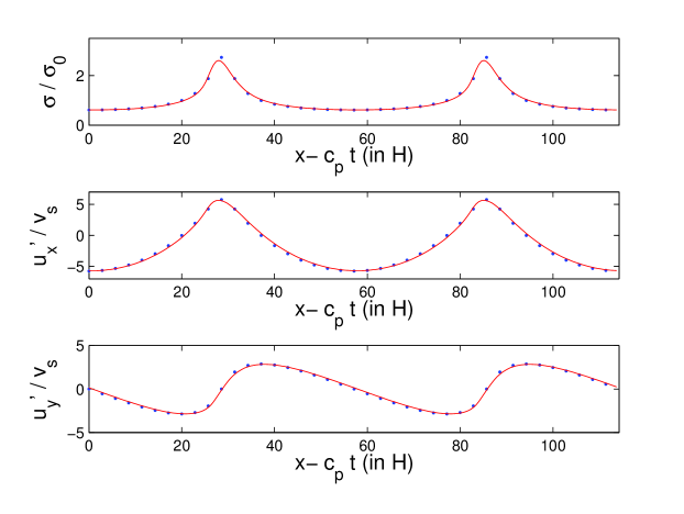
Figure 2: Two periods of a large amplitude wavetrain; both asymptotic and numerical solution are plotted. The solid curve is the numerical solution to (23)–(26), the points represents the asymptotic solution (31)–(35). Parameters correspond to $\tau=1.5$, as in Fig. 1, but now with $\mu=0.11$, so that $\lambda=57.1$.

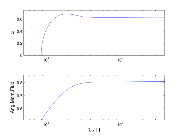
Figure 3: Panel (a) displays the scaled velocity amplitude of the nonlinear waves $q$ as a function of $\lambda=2\pi/\mu$. Near the critical wavelength, $q$ is almost zero and we are in the linear regime. From there it increases steeply and approaches a constant value, which agrees with the asymptotic $q$ computed from (35), $q_{0}=0.63339$. Panel (b) displays the total angular momentum flux. At amplitudes near criticality, the waves carry negligible amounts of angular momentum and the background shear flow dominates the transport. In contrast, larger amplitude wavetrains can carry appreciable amounts of up to a third of the background $3\alpha/2$. Recall $\alpha=0.342$.

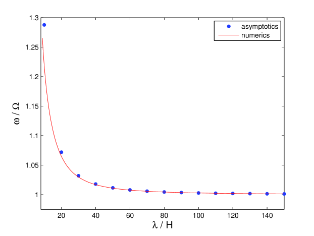
Figure 4: The nonlinear wavetrain frequency $\omega$ is graphed as a function of $\lambda$. The solid curves represent the numerical solution and the points the prediction of the asymptotic theory, (33).

Wavetrains with $\mu$ near $\mu_{c}$ possess small amplitudes, as is shown in Fig. 1. In this small amplitude ‘linear regime’ the solutions we compute connect, naturally, to the marginal linear overstable modes, which are necessarily sinusoidal.

As $\mu$ decreases ($\lambda$ increases) the nonlinear amplitudes increase. For sufficiently long wavelengths the self-similar asymptotic profiles of (31)—(35) provide a good approximation to the solutions, as we can see in Fig. 2. The profiles of these long waves resemble those of spiral density waves, as computed by Shu et al. (1985a, 1985b) and Borderies et al. (1983, 1986), and also axisymmetric density waves in accretion disks (Fromang and Papaloizou 2007). The characteristic ‘cusp’-like profile seems a recurrent feature of density waves dominated by the inertial forces.

In addition to these typical profiles we show how the scaled velocity amplitude $q$ varies with wavelength $\lambda=2\pi/\mu$ in Fig. 3a. Recall that the actual velocity amplitude is equal to $q/\mu$ (cf. Eq. (31)). By about $\lambda\approx 30\,H$ the amplitude $q$ begins to approach the value computed by the asymptotics, Eq. (35). For the parameters in which we are interested, the asymptotic result becomes an acceptable approximation for wavelengths above $20-30\,H$.

In Fig. 3b we plot the angular momentum flux density over one period in the wavetrain as a function of $\lambda$. We use the expression (30). The small amplitude waves transfer negligible angular momentum, so when $\mu\approx\mu_{c}$ the angular momentum flux is approximately that of the unperturbed disk, specifically $(3/2)\alpha$. Longer wavelength, larger amplitude wavetrains, however, can carry appreciable quantities above that of the background shear, but they may never exceed it. The angular momentum flux asymptotes to a constant value for large wavelengths, in agreement with the asymptotic theory.

Lastly, in Fig. 4 the eigenvalue $\omega$ is plotted against $\lambda$ for the same set of parameters. The longer the wavelength the closer the frequency is to the epicyclic with pressure ensuring the oscillations are a little faster. These behaviours are predicted by the asymptotic nonlinear dispersion relation which appears to provide an adequate approximation by about $\lambda\approx 30-40\,H$.

4.6 Discussion of neglected physics

The wave solutions have been computed by a relatively simple fluid model, but we feel that their existence and gross features are not captive to its assumptions. The asymptotic analysis shows that self-gravity (a collective effect) will not alter the leading order wave profiles. Self-gravity will, however, alter the nonlinear dispersion relation (33), adding a term proportional to $|\mu|$. Also, by exacerbating the linear viscous overstability it will ‘shift’ the curve in Fig. 3a to the left, which means that for a given $\lambda$ a wavetrain will be ‘more nonlinear’ (its amplitude will be greater) when self-gravity is present than when it is not. On the other hand, neglected thermal effects help stabilise the linear instability (Spahn et al. 2000) and so the curve in Fig. 3a may shift back to the right again. Thermal effects will also alter the pressure contribution to the nonlinear dispersion relation embodied by the function $F_{1}$.

It is more difficult to ascertain the effect of vertical structure and vertical motion on the solutions. The linear modes may be stabilised on intermediate scales due to their development of vertical shear (see Latter and Ogilvie 2006b), thus shifting Fig. 3a a little to the right. But because planetary rings are so very thin this is probably not important. There will be additional effects tied to the vertical motion, the ‘breathing’, which allied with excluded volume effects at wave peaks, could lead to the vertical ejection of particles and the relaxation of the pressure and stress in real planetary rings (‘splashing’). But how this plays out on moving wavecrests is difficult to forecast. The role of a nonlinear stress/strain relationship is also difficult to judge, though at the very least it will probably lead to greater effective $\beta$s and hence shift the $q$ curve to the right.

In summary, we have demonstrated the existence and elaborated on the properties of a family of exact nonlinear solutions to the governing equations (14)-(16). The solutions take the form of steady, travelling density waves propagating in either radial direction. They may also be regarded as fixed points or periodic orbits in the state space of the system. The members of this family can be distinguished by their wavenumber $\mu$ (or wavelength $\lambda$) upon which only one restriction holds, $\mu<\mu_{c}$, where $\mu_{c}$ is the critical wavenumber of linear viscous overstability. As such, an infinite number of solutions formally exist on arbitrarily long lengthscales; however above a certain lengthscale the model assumptions will certainly break down.

5 Linear stability of the nonlinear wavetrains

The question now is: what role do the nonlinear solutions play in the evolution of an overstable disk? To make a start on this we need to determine the linear stability of the nonlinear solutions themselves. If the system is to settle on a wavetrain then it must be at least linearly stable. On the other hand, if it is linearly unstable then we are assured that the system will not settle there (though this does not mean it plays no role in the dynamics). We find, in fact, that there exists a critical wavelength $\lambda_{\text{st}}$ above which linear stability is assured. Wavetrain solutions with $\lambda<\lambda_{\text{st}}$ are unstable and solutions with $\lambda>\lambda_{\text{st}}$ are stable.

These results are established by perturbing the wavetrain solution by a small disturbance and subsequently solving the eigenvalue problem that results for its growth rate. The procedure requires the solution of a Floquet boundary value problem which we attack analytically in the asymptotic limit of $0<\mu\ll 1$ (Appendix A) and numerically for general $\mu$.

5.1 The linear eigenvalue problem

Consider the wavetrain associated with $\mu$ and parameters $\alpha$, $\alpha_{b}$, and $\beta$. We denote this basic state by $\bm{Z}_{0}(\theta)=(\sigma_{0},u_{x0},u_{y0})(\theta)$, with the dependence on $\mu$ assumed. On this solution we superimpose a small disturbance so that

$$\bm{Z}=\bm{Z}_{0}(\theta)+\bm{Z}_{1}(t,\theta),$$

where $\|\bm{Z}_{1}\|\ll 1$. Upon substituting this ansatz into the governing equations (1)-(2), employing the definition (19), and linearising, the system returns the boundary value problem:

$$\partial_{t}\bm{Z}_{1}=\mathcal{L}_{0}(\theta)\,\bm{Z}_{1}$$ (36)

where $\mathcal{L}_{0}$ is a second-order differential operator in $\theta$ with $2\pi$-periodic coefficients.

Next we assume $\bm{Z}_{1}(t,\theta)=e^{st}\,\widetilde{\bm{Z}}_{1}(\theta)$ which reduces (36) to a Floquet eigenvalue problem for the growth rate $s$, owing to the periodicity of $\mathcal{L}_{0}$. In order to compute the spectrum we consequently make the Floquet ansatz,

$$\widetilde{\bm{Z}}_{1}=e^{i(k/\mu)\theta}\,\hat{\bm{Z}}_{1}(\theta),$$ (37)

where $\hat{\bm{Z}}_{1}$ is a $2\pi$ periodic function of $\theta$, the Floquet exponent is $(k/\mu)$, and $k$ is the (real) wavenumber of the envelope (both $s$ and $k$ are different to those appearing in Section 3). Once substituted back into (36), one can numerically solve the ensuing eigenproblem for $\hat{\bm{Z}}_{1}$ and the eigenvalue $s$ if the parameter $k$ is stipulated.

We now present the full set of linear equations governing the initial evolution of the small disturbances. Instead of rendering the problem in the form of Eq. (36), we express it as five simpler first-order differential equations for $\hat{\sigma}_{1}$, $\hat{u}_{1}=c_{p}-\hat{u}_{x1}$, $\hat{v}_{1}=\hat{u}_{y1}$, $\hat{f}_{1}$, and $\hat{h}_{1}$. This form facilitates the numerical calculation. The hats will now be dropped. The five ODEs are

$$\frac{d\sigma_{1}}{d\theta} =\frac{1}{u_{0}}\left[\left(\frac{s-iku_{0}}{\mu}-\frac{du_{0}}{d\theta}\right)\sigma_{1}-\left(\frac{d\sigma_{0}}{d\theta}+\frac{ik\sigma_{0}}{\mu}\right)u_{1}-\sigma_{0}\,\frac{du_{1}}{d_{\theta}}\right]\,,$$ (38)

$$\frac{du_{1}}{d\theta} =-\frac{ik}{\mu}\,u_{1}-(1+\beta)\,\frac{du_{0}}{d\theta}\,\frac{\sigma_{1}}{\sigma_{0}}-\frac{\sigma_{1}-f_{1}}{\mu(\alpha_{b}+\tfrac{4}{3}\alpha)\sigma_{0}^{1+\beta}}\,,$$ (39)

$$\frac{dv_{1}}{d\theta} =-\frac{ik}{\mu}\,v_{1}-(1+\beta)\,\frac{dv_{0}}{d\theta}\,\frac{\sigma_{1}}{\sigma_{0}}+\frac{\tfrac{3}{2}\alpha(1+\beta)\sigma_{0}^{\beta}\,\sigma_{1}-h_{1}}{\mu\alpha\sigma_{0}^{1+\beta}}\,,$$ (40)

$$\frac{df_{1}}{d\theta} =-\frac{ik}{\mu}\,f_{1}+\sigma_{0}\left[\left(\frac{s-iku_{0}}{\mu}-\frac{du_{0}}{d\theta}\right)\,u_{1}-u_{0}\,\frac{du_{1}}{d\theta}+\frac{2}{\mu}\,v_{1}+\frac{df_{0}}{d\theta}\,\frac{\sigma_{1}}{\sigma_{0}^{2}}\right]\,,$$ (41)

$$\frac{dh_{1}}{d\theta} =-\frac{ik}{\mu}\,h_{1}-\sigma_{0}\left[\frac{s-iku_{0}}{\mu}\,v_{1}-u_{0}\,\frac{dv_{1}}{d\theta}-\left(\frac{dv_{0}}{d\theta}+\frac{1}{2\mu}\right)\,u_{1}-\frac{dh_{0}}{d\theta}\,\frac{\sigma_{1}}{\sigma_{0}^{2}}\right],$$ (42)

and these hold on the domain $\theta\in[0,2\pi]$ subject to the periodic boundary conditions, $\sigma_{1}(0)=\sigma_{1}(2\pi)$, $u_{1}(0)=u_{1}(2\pi)$, etc. Before we undertake the calculation, we need to specify the material parameters $\alpha$, $\alpha_{b}$, $\beta$, the wavenumber of the underlying wavetrain $\mu$ (and hence the basic state $\bm{Z}_{0}$), and lastly the wavenumber of the disturbance $k$.

5.2 Numerical results

The equations for the equilibrium (22)-(26) and the linear stability (38)-(42) are solved simultaneously using the shooting method. We restrict the parameter values to those corresponding to optical depths of 1-2 and similar parameters. For these values we witness little qualitative change in the results. For more remote values, especially $\alpha_{b}/\alpha$ small or zero, we find different stability behaviour but this will not be presented here.

Once $\alpha$, $\alpha_{b}$, and $\beta$ are fixed, we investigate how the various linear modes depend on the wavenumber of the underlying wavetrain $\mu$, as a function of $k$. The reader should take care to distinguish between $\mu=2\pi/\lambda$, the wavenumber of the perturbed equilibrium, and $k$, the envelope wavenumber of the perturbation. Normally, one need only let $k$ vary between $0$ and $\mu/2$; values of $k$ outside this range merely reproduce modes already computed. However, in this section we let $k$ take values between $0$ and $\mu$. This choice lets us display and interpret the results in a clearer (and more familiar) way, while permitting us to connect the results directly with the homogeneous disk case.

The numerical solution establishes the existence of

• a ‘generalised’ viscous instability mode, which always decays at a rate proportional to $\alpha k^{2}$;

• two ‘generalised’ viscous overstability modes which can either grow or decay at a rate proportional to $\alpha k^{2}$ and which oscillate near the epicyclic frequency;

• modes which decay rapidly, at a rate of order $\alpha$ and which also oscillate at the epicyclic frequency.

The two modulational overstable modes appear as right-going and left-going waves. They generally possess different growth rates because the equilibrium background (a nonlinear wavetrain propagating either left or right) no longer supports the left/right symmetry exhibited by the homogeneous disk. We are primarily interested in these modes, as they are the only ones which are capable of growing. We refer to them as ‘modulational’ because they exist as long modulations of the phase and amplitude of the equilibrium wavetrains. Thus the fastest growing overstable modes possess wavelengths significantly longer than the wavelength of the equilibrium wavetrains.

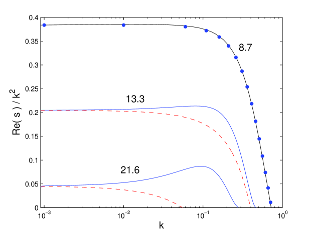
Figure 5: Real part of the scaled growth rate $s/k^{2}$ as a function of the wavenumber $k$ for modulational overstable modes. The solid lines correspond to the modes propagating against the underlying wavetrain; dashed lines correspond to modes propagating with. Three background equilibria are selected: nonlinear wavetrains with wavelengths $8.7$, $13.3$, $21.6$. The material parameters of the disk are taken from Table 1 for $\tau=1.5$. In addition, we plot the stability curve for the homogeneous equilibrium (from Eq. (10)) as points. The amplitude of the $\lambda=8.7$ nonlinear wavetrain is very small (being close to the critical wavelength) and thus the disk is in the linear regime of the homogeneous disk. Therefore the stability curve in these two cases agree. Larger $\lambda$ and wavetrain amplitudes impede modulational overstability. But modes propagating against the background wavetrain are more unstable than those propagating in the same direction. In the homogeneous disk the growth rates are the same.

First, in order to check the numerical results, we examined the stability of wavetrains of very small amplitude, i.e. those which possess a wavenumber $\mu$ near the critical value $\mu_{c}$. Recall that $\mu_{c}$ is the wavenumber of marginal viscous overstability (see Eq. (13)) and simultaneously of the very existence of nonlinear wavetrain solutions (see Fig. 3). In this limit the nonlinear wavetrain solution, being of small amplitude, can be simply absorbed into the perturbation field and the equilibrium treated as the homogeneous state. In this limit the growth rates for both the ‘generalised’ viscous instability and ‘generalised’ viscous overstability coincide exactly with their homogeneous disk counterparts (Eq. (10)), which provides the check on the numerics. The good agreement obtained between the two approaches is evident in Fig. 5 which plots the numerical growth rate of the modulational overstability, for the small amplitude wavetrain $\lambda=8.7$, alongside the analytic growth rate obtained from the homogeneous problem (10).

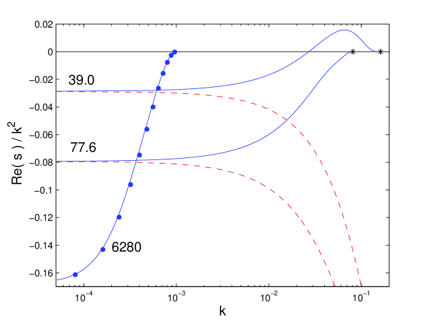
Figure 6: Continuation of Fig. 5. Real part of the scaled growth rate $s/k^{2}$ as a function of $k$ for the modulational overstable modes. We present results for three background wavetrains: $\lambda=39.0$, $\lambda=77.6$, and the very long $\lambda=6280$ case. The material parameters and notation are the same as the previous figure and the range of $k$ is $0$ to $\mu$. Stars indicate the point $k=\mu$ in both cases. The $\lambda=39.0$ graphs show the persistence of instability on intermediate $k$ for the counter-propagating mode, and stability for its oppositely moving twin. By $\lambda=77.6$ both modes have stabilised. In addition, we plot the prediction of the large $\lambda$ asymptotic theory (see Appendix A) as points, and find good agreement between it and the $\lambda=6280$ case.

Next we gradually increase the wavelength of the background wave $\lambda$ and check its stability at each step. Some of these results we present in Figs 5 and 6. These figures show the growth rates of the two modulational overstability modes as a function of $k$ for several representative wavetrains. The model parameters correspond to $\tau=1.5$ in Table 1. In the first figure, the stability of $\lambda=8.7$, $13.3$ and $21.6$ wavetrains are plotted, with the growth rate of the overstability mode propagating with the underlying wavetrain represented by the dashed line, and the growth rate of the mode propagating against by the solid line. As is plain, increasing the $\lambda$ of the background (a) impedes both modes’ growth and (b) breaks the left/right symmetry of the problem so that the dispersion relations of the two modes no longer coincide. In particular, growth of the countermoving mode is exacerbated on an intermediate range of $k$. In the limit of very small $k$ the growth rates of the two modes are the same.

From Fig. 6 we see that both modes stabilise when the underlying wavetrain is sufficiently long. Though the critical $\lambda$ at which this happens is different for the two modes (because of the exacerbated growth of the countermoving mode at intermediate $k$). For the parameters chosen, the modulational overstable mode travelling with the background stabilises when $\lambda\approx 27.0$ (or 119 m, using the dimensions of Table 1), while the countermoving mode stabilises when $\lambda\approx 52.8$ (or 234 m). We conclude that the nonlinear wavetrains’ stability criterion is controlled by the countermoving overstability mode. The critical wavelength above which a wavetrain is stable we denote by $\lambda_{\text{st}}$. And so sufficiently long wavetrains are linearly stable to all disturbances, which is in agreement with the asymptotic theory of Appendix A.

Lastly, the stability of very long wavetrains was checked so as to compare with the asymptotic linear stability and provide a second check on the numerics. In Sections A.4.1 a dispersion relation was computed giving the growth rate of the dominant modulational overstability mode. It is plotted with points in Fig. 6 against the prediction of the numerical eigensolution for a wavetrain with $\mu=0.001$. Though the agreement is good in this extreme case, the asymptotics provide an adequate approximation only for very long $\lambda$.

5.3 Summary

The linear theory is rather subtle and may repay extended study. For now, the essential point to take away is that there exist both linearly stable and linearly unstable wavetrain solutions. Wavetrains possessing a sufficiently long wavelength, namely $\lambda>\lambda_{\text{st}}$, are stable, while those that are shorter are unstable. The mode which governs the stability properties is the ‘modulational viscous overstability’, in particular, the mode which travels in the opposite direction to the underlying wavetrain. Those wavetrains that are unstable can be characterised as ‘saddle points’ in the phase space because they possess the unstable eigenmodes (the modulational overstabilities, which grow slowly, no faster than $\alpha k^{2}$), and a set of stable eigenmodes (some of which decay speedily, as $\alpha$).

This general behaviour is repeated for all realistic parameters we tried. If we turn to the parameters listed in Table 1, a ring with $\tau=1$ yields $\lambda_{\text{st}}=50.2$ (165 m), a ring with $\tau=1.5$ yields $\lambda_{\text{st}}=52.8$ (234 m), and a ring with $\tau=2$ yields $\lambda_{\text{st}}=117$ (640 m). The much longer value in the last case is due to the system’s sensitivity to the $\beta$ parameter. For fixed $\alpha$ and $\alpha_{b}$ we find that $\lambda_{\text{st}}$ is a steeply increasing function of $\beta$, a trend that is summarised in Table 3. The critical lengths at $\tau=1$-$1.5$ compare suggestively to the scales of quasi-periodic microstructure observed by Cassini, which are some 150-220 m (Colwell et al. 2007, Thomson et al. 2007). But it should be noted that important physics remains missing and the stability estimates are subject to some revision. In particular, the results for $\tau=2$, and greater $\beta$ generally, are probably blemished by neglect of certain physical processes (self-gravity, for example). Nevertheless, the overall consistency is encouraging.

$\beta$	$\lambda_{\text{st}}$ (in $H$)
1.1	41.9
1.19	52.8
1.3	71.0
1.4	91.7
1.5	121

Table 3: The critical $\lambda$ of stability for nonlinear wavetrains as a function of $\beta$. The other parameters $\alpha$ and $\alpha_{b}$ are held fixed: $\alpha=0.342$ and $\alpha_{b}=0.681$. The case $\beta=1.19$ corresponds to an optical depth of 1.5, larger values of $\beta$ correspond to more optically thick disks. For instance, the $\beta=1.5$ case is associated with $\tau=2$ (Schmidt et al. 2001).

6 General nonlinear dynamics

Armed with the linear stability results, we return to the question posed earlier: what role does this family of ‘fixed points’ play in the general dynamics of an overstable disk? The simplest outcome would be for an overstable disk to migrate from the homogeneous state to the shortest stable wavetrain solution (with $\lambda=\lambda_{\text{st}}$); but this is far from guaranteed. The dynamics is likely to be more complicated, with the system flirting with a number of stable nonlinear solutions and thus exhibiting irregular time and space dependent variations. In this section we explore this behaviour with some schematic ideas and analogies. We will not bury ourselves in technical details; this we leave for later, when we have a more complete set of numerical results at hand.

First, we offer an explanation of the cascade of power to longer lengths that has been observed in nonlinear hydrodynamical and $N$-body simulations. The analysis is framed in the language of dynamical systems theory and though ‘hand-wavey’ should be straightforward to check numerically. Next we examine the nonlinear interactions between linearly stable wavetrains of different wavelength, by computing slow variations in the wavetrains’ phase. It can be shown that the disk supports modulational ‘shock’ and ‘source’ structures, whereby the wavenumber and/or amplitude of a wavetrain undergoes a discontinuity. Lastly, we draw analogies between a viscously overstable disk and the dynamics of the complex Ginzburg-Landau equation, and subsequently make a few additional predictions about the likely nonlinear behaviours associated with overstable disks.

6.1 The cascade to longer lengthscales

In Fig. 7 we have drawn a schematic diagram of the state space of the overstable disk. The state space is infinite-dimensional, and, needless to say, somewhat difficult to visualise, but our crude two-dimensional projection raises a few interesting points and predictions. This representation of the dynamics treats the time-evolution of the state vector $\bm{Z}$ as a trajectory, tracing the smooth transition of the system from one state to another. Equilibria appear as invariant fixed points: trajectories that begin there stay there, and their linear stability decides if trajectories that pass infinitesimally close fall into the fixed point or are repelled. The state of homogeneous Keplerian shear is such a fixed point, and when it is overstable it behaves like a saddle. Nearby trajectories will be deflected away from the point along those directions associated with the overstability modes. Simultaneously, the same trajectories will be drawn towards the fixed point along those directions associated with the stable modes.

A nonlinear wavetrain solution should appear as a periodic orbit, but for clarity we represent it as a fixed point in Fig. 7; our argument is unchanged. The entire family of these nonlinear wave solutions plots out a semi-infinite, one-dimensional curve in the state space, which we parametrise by $\lambda$, the wavelength. The foot of this curve is the homogeneous state. In Fig. 7 the thick curve represents this continuous family of solutions, and the thinner arrowed curves represent possible trajectories of the system.

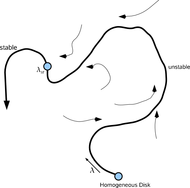
Figure 7: A schematic drawing showing a two-dimensional projection of the overstable disk’s state space, and the upward cascade to longer lengthscales. The thick curve represents the continuous family of nonlinear wavetrains, parametrised by $\lambda$, and the thin curves represent typical trajectories. Also plotted are the state of homogeneous Keplerian shear and the first stable nonlinear wavetrain, for which $\lambda=\lambda_{\text{st}}$. The basic idea is that trajectories repeatedly pass from the overstable manifold of one fixed point to the stable manifold of a neighbouring longer wavelength fixed point. This process ends, or at least undergoes a qualitative change, once the trajectory enters the vicinity of the first stable fixed point.

Waves are unstable if $\lambda<\lambda_{\text{st}}$, where $\lambda_{\text{st}}$ is some critical wavelength, while longer waves are stable, and like the overstable homogeneous state, the unstable wave solutions are saddles, each possessing a slow overstable manifold and a fast stable manifold. Trajectories near the unstable segment of the curve of fixed points will be drawn towards the curve along the nearest stable manifold; at the same time trajectories are directed ‘up’ the curve by the overstable manifold. Because the time-scale of the attraction is faster than that of repulsion, trajectories will be bunched, or ‘focused’, about the curve of fixed points even as they travel up it. Close to the branch of invariant fixed points this migration may be facilitated by the the linear ‘translation mode’ with $s=0$ and eigenvalue $\partial_{\theta}\bm{Z}_{0}$ (see next subsection). Thus the thick curve in Fig. 7 is a one-dimensional ‘spine’ around which collects a nest of state-space trajectories. Such behaviour is typical of dissipative systems, in which the long time dynamics is governed by a lower dimensional subset of the state space (e.g. Robinson 2001).

The upward drift will end, or at least change qualitatively, once a trajectory reaches the vicinity of the first stable fixed point. Because larger $\lambda$ fixed points are, necessarily, associated with longer wavelengths this upward migration should coincide with the movement of power to longer and longer scales.

It is not immediately obvious what happens once a trajectory nears the first stable fixed point, nor how a trajectory behaves if it begins near the stable portion of the solution branch. The simplest outcome is for the system to settle on the first stable fixed point available ($\lambda_{\text{st}}$ for example), but this is far from assured. The basin of attraction of a stable fixed point may be very small, and we expect this to be the case for most parameters. It is more likely that the system will ‘wander around’ the set of stable solutions, yet never fall upon any particular one. Physically this ‘wandering’ will appear as temporal and spatial modulations upon a bed of nonlinear waves, with the modulations manifesting on lengthscales longer than that of the underlying wavetrains. It is not clear which set of $\lambda$ the system will select for the underlying waves, or whether this set gradually changes (perhaps growing larger and larger with time). Moreover, the situation may be complicated by a chaotic attractor (as can be the case in the complex Ginzburg-Landau equation). That said, it is plausible that small initial conditions will yield a band of saturated wavelengths near $\lambda_{\text{st}}$.

These conjectures are straightforward to check with numerical simulations, and we are currently undertaking this work. The only published simulation, that of Schmit and Tscharnuter (1999), exhibited an upward cascade which in the nonself-gravitating case had not yet halted after $10,000$ orbits. By that stage most power was situated on a scale of some $100H$. According to the linear stability calculations of the previous section, using the same parameters as Schmit and Tscharnuter, we find $\lambda_{\text{st}}\approx 60H$; so the simulation definitely passed the critical wavelength of the linear analysis. Recall, however, that these simulations do not support global nonlinear wavetrain solutions on account of the boundary conditions and this negates much of the interpretation of this section. In their simulations, trains of travelling waves can emerge locally but given sufficient time (and 10,000 orbits is more than enough) these pulses will traverse the domain, encounter the boundaries, and reflect backwards and interfere with themselves. Such nonlinear interactions are not captured in our model and perhaps induce an injection of power to longer scales than what we would expect.

Finally, one should note that in our interpretation the halting of the upward cascade does not require self-gravity, which is an effect Schmit and Tscharnuter emphasise. In their simulations its inclusion halts the upward cascade. But it is probable that the physical mechanism is different to that we have sketched.

6.2 Modulated wavetrains: weak shocks, sources, and cellular dynamics

This and the next section ascertains the basic nonlinear dynamics of wavetrain modulations. This will give us some handle on the behaviour of the system once it nears the set of stable fixed points described in Fig. 7. The problem is a difficult one, and not generally amenable to analytic techniques. That said, a useful result can be derived if it is assumed that the modulations in question vary slowly in time and space. When this is the case, the phase perturbations are governed by the Burgers equation, which in turn suggests that the radial domain may fracture into regions (‘cells’) of different wavenumber bounded by two kinds of interface: ‘weak shocks’ and ‘weak sources’, where the phase undergoes rapid change. The actual dynamics is perhaps even more complicated than this ideal picture but it remains a useful paradigm to understand the larger-scale irregular variations observed. It is also worth remarking that the theory is akin to the attractive idea proposed by Tremaine (Araki and Tremaine 1986, Tremaine 2003) whereby disk structure corresponds to ‘jams’ — the key difference is that in the Tremaine model the jams correspond to discontinuities in shear, and in our model the jams correspond to discontinuities in the wavenumber of background waves.

We now very briefly describe the derivation of the Burgers equation. The proof is lengthy and tedious so more details can be found in Appendix B. It is essentially a multiple-scales analysis which applies the methodology of Howard and Kopell (1977) and Doelman et al. (2009) who examined modulated wavetrains in reaction–diffusion systems.

6.2.1 The Burgers equation

Consider a linearly stable wavetrain of $\mu$ and $\omega=\omega(\mu)$ when $\mu$ is small. We represent it by the vector $\bm{Z}_{0}(\theta\,;\,\mu)$, where we have made the dependence of $\bm{Z}_{0}$ on wavenumber $\mu$ explicit in contrast to Section 4. The wavetrain is assumed stable; therefore, associated with it are a set of decaying linear modes possessing negative growth rates. Of these we select the modulational viscous instability mode and denote its growth rate by $s(k)$ where $k$ is its wavenumber. From Section 5 and Eq. (103), this mode always decays as $k^{2}$.

Slowly varying modulations of $\bm{Z}_{0}$ are sought. First we establish the long length and time scales characteristic of this modulation. For a small dimensionless parameter $0<\delta\ll 1$, define new (slow) variables

$$X=\delta(x-c_{g}\,t),\qquad T=\delta^{2}\,t,$$

where $c_{g}$ is the group velocity of the underlying wavetrain:

$$c_{g}\equiv\frac{d\omega}{d\mu}.$$

Note that we have chosen a spatial frame moving with the group velocity. Wavetrain modulations travel at $c_{g}$, not the phase velocity $c_{p}$.

Next a perturbation of the wavetrains’ phase is introduced, $\Theta(X,T)$. The associated variation in wavenumber is $\partial_{X}\Theta$. We now construct a solution of the form

$$\bm{Z}=\bm{Z}_{0}\left(\theta+\Theta\,;\,\mu+\delta\,\Theta_{X}\right)+\delta^{2}\,\bm{Z}_{1}(\theta,X,T),$$ (43)

where a subscript $X$ (or $T$) indicates partial differentiation. Our strategy is to derive an equation for the phase modulation $\Theta$ so that the ansatz (43) satisfies the nonlinear equations to the leading orders in $\delta$.

The ansatz (43) is substituted into (14)–(18) and these equations are expanded in powers of the small parameter $\delta$. At leading order $\delta^{0}$ the balance becomes the nonlinear eigenproblem for the underlying wavetrain profile, Eqs (23)–(26). At the next order $\delta^{1}$ the balance is a simple identity: the first $\mu$ derivative of the leading order equations. At order $\delta^{2}$ we obtain

$$\mathcal{L}_{0}\,\bm{Z}_{1}=-(\partial_{\theta}\bm{Z}_{0})\,\Theta_{T}+\bm{A}(\theta)\,\Theta_{XX}-\bm{B}(\theta)\,\Theta_{X}^{2},$$ (44)

where $\mathcal{L}_{0}$ is the linear operator introduced in Section 5, the $\bm{A}$ and $\bm{B}$ are vectors that depend only on the underlying wavetrain and so depend only on $\mu$ and $\theta$. Their expressions are complicated and we omit them here (see Appendix B). The order $\delta^{2}$ equation need only yield a solvability condition: the right side of Eq. (44) must lie in the range of $\mathcal{L}_{0}$ (the Fredholm alternative). This can be assured if the inner product of the right side with the adjoint solution of $\mathcal{L}_{0}$ is zero. After some laborious manipulation, the condition is equivalent to the Burgers equation,

$$K_{T}+\omega^{\prime\prime}(\mu)\,K\,K_{X}+\tfrac{1}{2}s^{\prime\prime}(0)\,K_{XX}=0,$$ (45)

where $K\equiv\Theta_{X}$ is the wavenumber modulation, and

$$\omega^{\prime\prime}(\mu)\equiv\frac{d^{2}\omega}{d\mu^{2}},\qquad\ s^{\prime\prime}(k)\equiv\frac{d^{2}s}{dk^{2}}.$$

The ‘phase diffusion coefficient’ is $-s^{\prime\prime}(0)/2$ and is associated with the decaying modulational viscous instability. Localised disturbances which ‘bunch up’ the crests of wavetrains will relax according to this mode. The ‘advective coefficient’ is $\omega^{\prime\prime}$ and thus equal to the group velocity’s rate of change with $\mu$. It controls the steepening of fronts or shocks in $K$. If $c_{g}$ is independent of $\mu$ there is no wave steepening. How one derives $s^{\prime\prime}(0)$ from $\bm{A}$ and $\omega^{\prime\prime}(k)$ from $\bm{B}$ is nontrivial and is left to Appendix B. There we also show how to compute the coefficients in terms of the material properties of the disk, $\alpha$, $\alpha_{b}$, and $\beta$.

6.2.2 Weak shocks and sources

For our purposes, equation (45) predicts two basic behaviours. Localised solutions $K(X,T)$ will decay to zero as $T\to\infty$ while propagating at a speed equal to the group velocity (Whitham, 1974, Doelman et al. 2009). This behaviour simply expresses the linear stability of the underlying wavetrain. Nonlocalised solutions, on the other hand, can manifest as viscous Lax shocks. For instance, suppose that we require

$$K\to K_{+}\quad\text{as}\quad X\to\infty,$$

$$K\to K_{-}\quad\text{as}\quad X\to-\infty,$$

where $K_{+}$ and $K_{-}$ are two real constants. Then Eq. (45) admits a travelling front or shock solution $K(X,T)=K_{\text{sh}}(X-c_{\text{sh}}\,T)$ when

$$\omega^{\prime\prime}(\mu)(K_{+}-K_{-})<0.$$ (46)

From Fig. 4 or from Eqs (33) and (34) we have $\omega^{\prime\prime}>0$ and thus $K_{+}<K_{-}$. In addition, the speed of the front is given by

$$c_{\text{sh}}=\tfrac{1}{2}\omega^{\prime\prime}(\mu)\,(K_{+}+K_{-}),$$

which is the Rankine-Hugoniot condition in the moving frame. The characteristics associated with the solution point towards the front interface, as do the motions of the individual wavecrests on its each side. Solutions for which the characteristics and wavecrests point away do not satisfy (46) and correspond to rarefaction waves or ‘sources’. Fig. 8 presents a cartoon of a nonlinear wavetrain exhibiting both a shock and a source at which points the wavenumber (and amplitude) rapidly change.

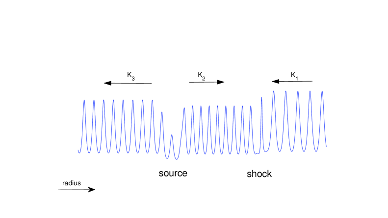
Figure 8: A simple cartoon representing a wavetrain with a shock and a source solution. The arrows represent the direction that the individual wavecrests propagate (the $c_{p}$), while $K$ represents the modulational wavenumber. Here $K_{1}<K_{3}<K_{2}$ are constants, and thus the defects ‘glue’ together patches of different wavenumber (and hence amplitude). On sufficiently large scales a wavetrain may decompose into a number of subtrains each possessing varying wavenumber and each enclosed by a shock and a source. These interfaces will possess their own slow dynamics — they may wander around the domain, annihilate one another, generate new defects, etc.

6.2.3 Cellular structure

In general reaction-diffusion systems, widely-spaced sources and shocks can partition the domain into distinct regions inhabited by wavetrains of different $\mu$ (Aranson and Kramer 2002, Doelman et al. 2009). Figure 8 roughly sketches a portion of a domain so decomposed. Similar phenomena should emerge in overstable disks, and it is possible that observed radial structure on intermediate scales in Saturn’s rings corresponds to the cellular patterns constructed from such wave defects.

Shock and souce interfaces will possess their own slow dynamics which compels them to drift relative to each other and undergo various kinds of interactions. The former motions may be represented by a simple one-dimensional ‘cellular’ dynamical system that evolves the interfaces according to a set of ordinary differential equations (Elphick et al. 1990, Ei 2002, Doelman et al. 2009). Each interface is treated as a particle that weakly interacts with its neighbours via a ‘potential’ and thus the model bears a similarity to a one-dimensional $N$-body problem.

Unfortunately, it is difficult to produce analytic estimates for the characteristic lengthscales of the cellular structures so formed. Thus comparison with Cassini data must wait. In any case, the model assumes only weak interactions between the interfaces, but full numerical simulations of the complex Ginzburg-Landau equation typically exhibit more complicated behaviour (Popp et al. 1993, Chaté 1994). We briefly survey these phenomena in the next subsection.

6.2.4 The complex Ginzburg-Landau equation

The complex Ginzburg-Landau equation in an extended domain boasts a substantial literature, equal to the diverse behaviour it exhibits. This body of work may guide the interpretation of future nonlinear simulations of the overstability. The complex Ginzburg-Landau system crystallises the essential dynamics of general nonlinear wave phenomenon in a broad range of physical situations (Aranson and Kramer 2002) and which we expect nonlinear waves in planetary rings to share.

The one-dimensional version of the equation reads

$$\partial_{t}A=A+(1+ic_{1})\partial_{x}^{2}A-(1+ic_{2})|A|^{2}\,A,$$

where $A$ is a complex function and $c_{1}$ denotes the linear dispersion and $c_{2}$ nonlinear dispersion. The function $A$ typically represents the complex amplitude of some wave phenomenon, and is not the same as the phase modulation $\Theta$ which we studied earlier — the latter, though, can be derived from $A$. The equation gives rise to steady, nonlinear wavetrains, various wave instabilities, and ‘defects’ (such as source and shock structures) that can ‘glue’ together different wavetrains, in addition to different types of spatio-temporal chaos (Aranson and Kramer 2002).

Of the various regimes exhibited, behaviour associated with the so-called ‘intermittency regime’ is of most interest. Here the state space admits not only stable nonlinear wavetrain solutions but also a ‘defect-turbulent attractor’ (Chaté 1994). The role of the latter is to govern the irregular dynamics of the shocks and sources that separate the different regions of stable travelling waves. A number of studies have explored the rich and chaotic dynamics of the interfaces (Popp et al. 1993, Chaté 1994, Ipsen and Hecke 2001): for instance, source and shock structures may wander around the domain, annihilate each other, and give birth to new shock and source pairs. The long-time outcome is also variable, and depends closely on the parameters. For certain choices of $c_{1}$ and $c_{2}$, the final state may be ‘glassy’ (a static arrangement of defects), the defects may evaporate altogether, or the birth and annihilation process continues indefinitely. Another interesting regime is that of ‘phase chaos’ in which the wavenumber of the nonlinear wavetrains undergo turbulent fluctuations. All or some of this behaviour we expect to carry over to the dynamics of the overstable disk. At the very least, the complex Ginzburg-Landau equation provides a template with which to interpret simulations of overstable disks and the ISS observations of irregular structure in the B-ring.

7 Conclusion

This paper has investigated the dynamics of an overstable fluid disk by exploiting the properties of its nonlinear invariant solutions. These structures manifest as axisymmetric uniform travelling wavetrains and form a continuous family of solutions parametrised by their wavelength $\lambda$. In Section 4 and Appendix A we computed the members of this family and outlined their physical characteristics. In particular, we find that inertial forces dominate their leading order force balance, and so the fluid undergoes approximately epicyclic motion. The wave amplitudes, on the other hand, are determined from an energy balance that counterpoises linear viscous overstability and viscous dissipation. In Section 5 the wavetrains’ stability to small perturbations is inspected. It turns out that only solutions with wavelengths above a critical value $\lambda_{\text{st}}$ are linearly stable. If the viscous parameters take values associated with Saturn’s B-ring, $\lambda_{\text{st}}\approx 50-100\,H$. Finally, in Section 6 we speculate on the role of the nonlinear wavetrains in the general dynamics, arguing that the system will linger ‘near’ the branch of linearly stable invariant solutions. Physically, this phase-space behaviour will translate to a bed of nonlinear waves suffering large-scale modulations or defects, the latter partitioning the domain into a cellular grid of wavetrains of different $\lambda$.

Our basic hypothesis is that quasi-periodic microstructure on scales of order $100$m revealed by the UVIS and RSS correspond to the underlying bed of nonlinear waves. Meanwhile, irregular structure on larger scales, of 500m to 10km may be a manifestation of the wavetrains’ spatio-temporal modulations, arising as the system flirts with a number of stable wavetrain solutions but is unable to settle on any. The individual waves are beneath the ISS cameras’ resolution, but larger-scale variations in their amplitude and wavelength should give rise to different optical properties which the cameras can register. In order to fully establish the latter point, however, the optical properties of the nonlinear waves need to be understood. The dynamical and photometric modelling techniques that have been developed to understand the observational properties of gravitational wakes could be applied to this end (French et al. 2007, Colwell et al. 2007).

This study has adopted some rather strong modelling assumptions and neglected some important physics. The issue requiring the most urgent attention is self-gravity, as it will certainly play a role in the formation and stability of the nonlinear waves studied. Its effects we examine in a following paper. The 1D isothermal fluid model we have employed is simple, but we doubt that the basic physics it has revealed is an artefact of its simplicity. That said, on at least two counts it can be improved: first, its treatment of the viscous stress, and second, its neglect of vertical motion. The Navier–Stokes stress prescription is not ideal in a scenario of densely-packed and infrequently colliding particles, where the collisional stress dominates. A detailed kinetic treatment is perhaps the best way to capture the nonlinear dependence on strain associated with a collisional stress (Latter and Ogilvie 2008). Vertical motions, such as ‘breathing’ or ‘splashing’, certainly accompany both the linear modes of the viscous overstability and its nonlinear development (Salo et al. 2001, Latter and Ogilvie 2006b). The importance of this effect is difficult to judge; and may only be resolved by 2D eigensolutions and simulations, both formidable tasks.

Lastly, we briefly sketch out future work. Once the role of self-gravity on the nonlinear waves has been established, large-scale hydrodynamical simulations of an overstable ring must be undertaken to test our various conclusions. These should also address the influence of the boundary conditions, which will help us connect the work here to that of Schmit and Tscharnuter (1999). On the other hand, the dense–gas kinetic equations may be simulated, using perhaps the continuum model derived by Latter and Ogilvie (2008). These then could provide a more direct comparison with $N$-body simulations and possibly to the observations of finescale structure themselves.

8 Appendix A: Asymptotic description of ring dynamics in the limit of small collective effects

The analysis presented in this appendix resembles earlier work on nonlinear waves in disks. Several papers by Shu and collaborators formulate equations for nonlinear spiral density waves in planetary rings and accretion discs (the most pertinent being Shu et al. 1985a, 1985b). They include self-gravity, pressure and viscous (or kinetic) stresses. However, they do not consider time-evolution or viscous overstability because they are interested in forced rather than free waves. The streamline formalism of Borderies et al. (1983, 1986) is closely related. They derive their equations using methods of celestial mechanics but the outcome is similar. Because they consider discrete streamlines rather than a continuous medium, they obtain coupled ODEs rather than PDEs which means that density waves are not so clearly manifested in their approach. Our analysis is intentionally restricted to axisymmetry and local geometry, which slightly clarifies matters and allows viscous overstability to take centre stage. The physics of self-gravity, nonaxisymmetry, and the gravitational influence of external moons may be included later.

8.1 Basic equations

We consider axisymmetric motions in a shearing sheet with no vertical extension. The sheet is Keplerian and units are chosen such that $\Omega=1$. The basic equations are

$$\mathrm{D}u-2v=\epsilon T_{x},$$ (47)

$$\mathrm{D}v+\frac{1}{2}u=\epsilon T_{y},$$ (48)

$$\mathrm{D}\sigma+\sigma\partial_{x}u=0,$$ (49)

where $\mathrm{D}=\partial_{t}+u\partial_{x}$ is the Lagrangian derivative, $T_{x}$ and $T_{y}$ are the radial and azimuthal accelerations due to the weak collective effects of pressure, viscosity, and self-gravity, and $\epsilon$ is an ordering parameter. Note that the notation here is different to the main body of the paper: $u$ denotes the radial velocity and $v$ the azimuthal velocity.

We anticipate that the dominant motion of fluid elements is an epicyclic oscillation of the form

$$x=\xi+a(\xi,t)\cos[t-b(\xi,t)],$$ (50)

where $a$ and $b$ are the epicyclic amplitude and phase, and $\xi$ is an approximate Lagrangian variable. It is not an exact Lagrangian variable because the exact motion of a fluid element in a viscous disk departs marginally from epicycles. In fact, we use this equation to define $\xi(x,t)$, and then determine how $a$ and $b$ must evolve so that this equation continues to describe the dominant motion of the fluid. This constraint is meaningful only if $a$ and $b$ evolve slowly in time, a constraint enforced by the asymptotic analysis below. We write $a_{\xi}$ and $a_{t}$ to represent $\partial a/\partial\xi$ and $\partial a/\partial t$, respectively. We also work with the complex epicyclic amplitude

$$A=ae^{ib}.$$ (51)

The relation between $x$ and $\xi$ is one-to-one provided that $|A_{\xi}|<1$. Interpenetration of neighbouring fluid elements (or streamlines) occurs if $|A_{\xi}|>1$.

We now change variables from $(x,t)$ to $(\xi,t)$, finding

$$\mathrm{D}u-2v=\epsilon T_{x},$$ (52)

$$\mathrm{D}v+\frac{1}{2}u=\epsilon T_{y},$$ (53)

$$\mathrm{D}\sigma+\sigma J^{-1}\partial_{\xi}u=0,$$ (54)

where now

$$\mathrm{D}=\partial_{t}+\tilde{u}J^{-1}\partial_{\xi},$$ (55)

$$\tilde{u}=u-\dot{x},$$ (56)

$$J=\left(\frac{\partial x}{\partial\xi}\right)_{t}=1+a_{\xi}\cos(t-b)+ab_{\xi}\sin(t-b),$$ (57)

$$\dot{x}=\left(\frac{\partial x}{\partial t}\right)_{\xi}=a_{t}\cos(t-b)-a(1-b_{t})\sin(t-b).$$ (58)

(Note that $\partial_{t}$ now denotes a derivative at constant $\xi$.) $J$ is the Jacobian (stretching factor) of the transformation between $x$ and $\xi$, while $\dot{x}$ is the radial velocity of a particle having constant $\xi$. If $\xi$ were an exact Lagrangian variable, then $u$ would equal $\dot{x}$, therefore $\tilde{u}$ is the radial velocity relative to the moving coordinate system. Note the identity

$$\partial_{t}J=\partial_{\xi}\dot{x}.$$ (59)

8.2 Asymptotic solution

We propose that $a$ and $b$ evolve, due to weak collective effects, on a timescale that is long (by a factor of order $\epsilon^{-1}$) compared to the orbital timescale. Thus $a$ and $b$ are considered as functions of $(\xi,\tau)$, where $\tau=\epsilon t$ is a slow time variable, and $a_{t}$ becomes $\epsilon a_{\tau}$, etc.

The solution is expanded in the form

$$\tilde{u} =\epsilon\tilde{u}_{1}+\cdots,$$

$$v =v_{0}+\epsilon v_{1}+\cdots,$$

$$\sigma =\sigma_{0}+\epsilon\sigma_{1}+\cdots,$$

where $\tilde{u}_{1}$, etc., are functions of $(\xi,t,\tau)$. (Note that these functions are different to those appearing in Section 5.1 though the notation is the same.) The multiple-scale analysis is necessary in order to separate the fast epicyclic oscillation from the slow evolution of the epicyclic amplitude and mass distribution. All the variables should be periodic functions of $t$ with period $2\pi$; any secular evolution is described by the dependence on $\tau$.

Note that $a$ and $b$ are not expanded in powers of $\epsilon$, because they represent only the leading-order motion. Thus $J(\xi,t,\tau)$ is a quantity of order unity and does not require expansion. On the other hand $\dot{x}$ contains terms of orders $\epsilon^{0}$ and $\epsilon^{1}$. The relation between $u$ and $\tilde{u}$ is

$$u-\tilde{u}=\dot{x}=-a\sin(t-b)+\epsilon[a_{\tau}\cos(t-b)+ab_{\tau}\sin(t-b)]=\dot{x}_{0}+\epsilon\dot{x}_{1}.$$

The identity (59) becomes

$$\partial_{t}J=\partial_{\xi}\dot{x}_{0},\qquad\partial_{\tau}J=\partial_{\xi}\dot{x}_{1}.$$ (60)

At leading order we have the epicyclic motion

$$\dot{x}_{0}=-a\sin(t-b),\qquad v_{0}=-\frac{1}{2}a\cos(t-b).$$ (61)

This satisfies the equations of motion (52) and (53) at $O(1)$. The equation of mass conservation (54) at $O(1)$ gives

$$\partial_{t}\sigma_{0}+\sigma_{0}J^{-1}\partial_{\xi}\dot{x}_{0}=0.$$ (62)

Multiplying by $J$ and using the identity (60), we obtain

$$\partial_{t}(\sigma_{0}J)=0,$$ (63)

which expresses conservation of mass on the epicyclic timescale. We may write $\sigma_{0}J=\Sigma(\xi,\tau)$.

Our task now is to deduce evolutionary equations for the epicyclic amplitude $A(\xi,\tau)$ and the epicycle-averaged surface density $\Sigma(\xi,\tau)$. (Note that, since $dx=J\,d\xi$ at fixed $t$, $\Sigma$ is really a density with respect to the $\xi$ coordinate.)

8.2.1 Evolution equations

The equation of mass conservation at $O(\epsilon)$ is

$$\partial_{t}\sigma_{1}+(\partial_{\tau}+\tilde{u}_{1}J^{-1}\partial_{\xi})\sigma_{0}+\sigma_{0}J^{-1}\partial_{\xi}(\tilde{u}_{1}+\dot{x}_{1})+\sigma_{1}J^{-1}\partial_{\xi}\dot{x}_{0}=0.$$ (64)

Multiplying by $J$ and using the identity (60), we find

$$\partial_{t}(\sigma_{1}J)+\partial_{\tau}(\sigma_{0}J)+\partial_{\xi}(\sigma_{0}\tilde{u}_{1})=0.$$

We now apply the epicyclic averaging operation

$$\langle\cdot\rangle=\frac{1}{2\pi}\int_{0}^{2\pi}\,\cdot\,dt,$$

to obtain

$$\partial_{\tau}\Sigma+\partial_{\xi}(\Sigma V)=0.$$ (65)

where $V(\xi,\tau)$ is a mean radial velocity defined by the averaged mass flux density

$$\Sigma V=\langle\sigma_{0}\tilde{u}_{1}\rangle=\Sigma\langle\tilde{u}_{1}J^{-1}\rangle.$$ (66)

What we have done here is to obtain an evolutionary equation for $\Sigma$ by applying a solvability condition that eliminates the unknown $\sigma_{1}$.

The equations of motion at $O(\epsilon)$ are

$$\partial_{t}(\tilde{u}_{1}+\dot{x}_{1})+(\partial_{\tau}+\tilde{u}_{1}J^{-1}\partial_{\xi})\dot{x}_{0}-2v_{1}=T_{x},$$ (67)

$$\partial_{t}v_{1}+(\partial_{\tau}+\tilde{u}_{1}J^{-1}\partial_{\xi})v_{0}+\frac{1}{2}(\tilde{u}_{1}+\dot{x}_{1})=T_{y}.$$ (68)

Our aim is to eliminate the unknowns $\tilde{u}_{1}$ and $v_{1}$ by obtaining a solvability condition that will provide an evolutionary equation for the epicyclic amplitude $A$. We will show how this can be obtained in a systematic manner. Let us rewrite the equations, noting that $\partial_{\xi}v_{0}=(1-J)/2$ and $\partial_{\tau}v_{0}=-\dot{x}_{1}/2$, in the form

$$\partial_{t}\tilde{u}_{1}+\frac{\tilde{u}_{1}}{J}\partial_{t}J-2v_{1} =\tilde{T}_{x}\,\equiv\,T_{x}-\partial_{t}\dot{x}_{1}-\partial_{\tau}\dot{x}_{0},$$

$$\partial_{t}v_{1}+\frac{\tilde{u}_{1}}{2J} =T_{y}.$$

The latter (angular momentum) equation, when averaged, gives us immediately

$$V=2\langle T_{y}\rangle.$$ (69)

Now eliminate $\tilde{u}_{1}$ between the two equations to obtain

$$-2Jv_{1}-2\partial_{t}(J^{2}\partial_{t}v_{1})=J\tilde{T}_{x}-2\partial_{t}(J^{2}T_{y})$$

On the left-hand side we have a linear operator in self-adjoint form acting on $v_{1}$. It can be verified that $J^{-1}e^{it}$ is a null eigenfunction. The corresponding solvability condition is

$$\langle J^{-1}e^{it}[J\tilde{T}_{x}-2\partial_{t}(J^{2}T_{y})]\rangle=0.$$ (70)

After an integration by parts and use of the identity

$$i\partial_{t}J=1-J+A_{\xi}e^{-it}$$

we have

$$\langle e^{it}\tilde{T}_{x}+2i(e^{it}+A_{\xi})T_{y}\rangle=0,$$

and so

$$\partial_{\tau}A+V\partial_{\xi}A=\langle e^{it}(iT_{x}-2T_{y})\rangle.$$ (71)

In summary, we have derived the evolutionary equations

$$\partial_{\tau}\Sigma+\partial_{\xi}(\Sigma V)=0,$$ (72)

$$\partial_{\tau}A+V\partial_{\xi}A=\langle e^{it}(iT_{x}-2T_{y})\rangle,$$ (73)

with

$$V=2\langle T_{y}\rangle.$$ (74)

The evolution of the mass distribution and the nonlinear waves are coupled together. We can now remove the ordering parameter and replace $\partial_{\tau}$ by $\partial_{t}$ here if desired. However, it is important to retain the conceptual distinction between the fast and slow timescales.

8.3 Evaluation of the force averages

8.3.1 Stress tensors in general

If the forces derive from a (two-dimensional/vertically integrated) stress tensor, then

$$T_{x}=-\frac{1}{\sigma}\partial_{x}f,\qquad T_{y}=-\frac{1}{\sigma}\partial_{x}h,$$

where $f$ and $h$ are as given in Sections 3 and 4 in the case of a fluid with an isotropic pressure and a Navier-Stokes viscous stress. Self-gravity is omitted. To calculate the stresses to leading order, we replace $\sigma$ with $\sigma_{0}$ here and use the leading-order velocity field where required. Also, noting that $\sigma_{0}^{-1}\partial_{x}=\Sigma^{-1}\partial_{\xi}$ and that $\Sigma$ is independent of the fast time $t$, we have

$$\langle e^{it}(iT_{x}-2T_{y})\rangle=-\frac{1}{\Sigma}\partial_{\xi}\langle e^{it}(if-2h)\rangle,$$ (75)

$$\langle T_{y}\rangle=-\frac{1}{\Sigma}\partial_{\xi}\langle h\rangle.$$ (76)

8.3.2 Pressure

We first compute the pressure contribution to the evolutionary equations by setting the viscous stress to zero. In the case of an isothermal gas with (two-dimensional/vertically integrated) pressure $p=v_{s}^{2}\sigma$, we have

$$f=v_{s}^{2}\Sigma J^{-1},\qquad h=0.$$ (77)

We must then evaluate $\langle e^{it}J^{-1}\rangle$. Let

$$A_{\xi}=(a_{\xi}+iab_{\xi})e^{ib}=qe^{i\phi}.$$ (78)

Here $0\leq q<1$ is the usual nonlinearity parameter for density waves in planetary rings (see Borderies, Goldreich, and Tremaine 1983, 1985, 1986). Then

$$J=1+\mathrm{Re}[A_{\xi}e^{-it}]=1+\mathrm{Re}[qe^{-i(t-\phi)}]=1+q\cos(t-\phi)=1+q\cos\theta$$

and

$$\langle e^{it}J^{-1}\rangle=e^{i\phi}\langle e^{i\theta}(1+q\cos\theta)^{-1}\rangle=e^{i\phi}\frac{1}{2\pi}\int_{0}^{2\pi}\cos\theta(1+q\cos\theta)^{-1}\,d\theta,$$

where $\theta=t-\phi$. This is straightforward to integrate and the evolutionary equations with pressure alone become

$$\partial_{t}\Sigma=0,$$ (79)

$$\partial_{t}A=\frac{iv_{s}^{2}}{\Sigma}\partial_{\xi}\left[F_{1}(q)\,\Sigma\,A_{\xi}\right],$$ (80)

with

$$F_{1}(q)=q^{-2}\,\left[(1-q^{2})^{-1/2}-1\right].$$ (81)

This is a type of nonlinear Schrödinger equation. Note that $q^{2}=|A_{\xi}|^{2}$.

8.3.3 Viscosity

Next we compute the contribution from viscosity alone, in the absence of pressure. Then

$$f=-(\nu_{b}+{\textstyle\frac{4}{3}}\nu)\sigma\partial_{x}u,\qquad h=-\nu\sigma(-{\textstyle\frac{3}{2}}+\partial_{x}v),$$ (82)

and we adopt the viscosity laws

$$\nu=\frac{v_{s}^{2}}{\Omega}\,\alpha\left(\frac{\sigma}{\sigma_{*}}\right)^{\beta},\qquad\nu_{b}=\frac{v_{s}^{2}}{\Omega}\,\alpha_{b}\left(\frac{\sigma}{\sigma_{*}}\right)^{\beta},$$ (83)

where $\sigma_{*}$ is a constant reference density. To leading order and in terms of the variables $Q=qe^{i\phi}$ and $\theta=t-\phi$ introduced previously,

$$f=v_{s}^{2}\,(\alpha_{b}+{\textstyle\frac{4}{3}}\alpha)\sigma_{*}\left(\frac{\Sigma}{\sigma_{*}}\right)^{\beta+1}J^{-\beta-2}q\sin\theta,$$ (84)

$$h=v_{s}^{2}\,\alpha\sigma_{*}\left(\frac{\Sigma}{\sigma_{*}}\right)^{\beta+1}J^{-\beta-2}({\textstyle\frac{3}{2}}+2q\cos\theta).$$ (85)

The weighted averages of these relations, which appear in Eqs (72)–(74), are complicated integral functions which may be rewritten in terms of associated Legendre functions. In summary,

$$\langle e^{it}(if-2h)\rangle=-\sigma_{*}v_{s}^{2}\,\left(\frac{\Sigma}{\sigma_{*}}\right)^{1+\beta}F_{2}(q)\,A_{\xi},$$ (86)

$$\langle h\rangle=-\sigma_{*}v_{s}^{2}\,\left(\frac{\Sigma}{\sigma_{*}}\right)^{1+\beta}F_{3}(q),$$ (87)

where we have introduced two new $F$ functions defined through

$$F_{2}(q) =\frac{(\widetilde{q})^{2+\beta}}{\beta(1+\beta)\,\,q}\left\{(\alpha_{b}+\tfrac{16}{3}\alpha)\frac{1}{\widetilde{q}}\,\text{P}^{(1)}_{\beta}(\widetilde{q})-3\alpha\beta\,\text{P}^{(1)}_{1+\beta}(\widetilde{q})+4\alpha\,q\,\text{P}^{(2)}_{1+\beta}(\widetilde{q})\right\}$$ (88)

$$F_{3}(q) =-\frac{\alpha\,\widetilde{q}^{2+\beta}}{1+\beta}\,\left\{3(1+\beta)\,\text{P}^{(0)}_{1+\beta}(\widetilde{q})-4q\,\text{P}^{(1)}_{1+\beta}(\widetilde{q})\right\},$$ (89)

where $\widetilde{q}=(1-q^{2})^{-1/2}$, a notational convenience, and $\text{P}^{(m)}_{\eta}$ is the associated Legendre function of the first kind and type 3. It is defined through

$$\text{P}^{(m)}_{\eta}(z)=\frac{\Gamma(m-\eta)}{\pi\Gamma(\eta)}\int_{0}^{\pi}\cos(m\theta)\left[z+\sqrt{z^{2}-1}\cos\theta\right]^{-\eta-1}\,d\theta$$

(see http://functions.wolfram.com/HypergeometricFunctions/LegendreP3General).

8.3.4 Combined evolutionary equations

Dimensions are adopted so that $v_{s}=1$ and $\sigma_{*}=1$. Finally, we arrive at a problem of the form

$$\partial_{t}\Sigma+\partial_{\xi}(\Sigma V)=0,$$ (90)

$$\partial_{t}A+V\partial_{\xi}A=\frac{1}{\Sigma}\,\partial_{\xi}\left\{\left[iF_{1}(q)+\Sigma^{\beta}F_{2}(q)\right]\,\Sigma\,A_{\xi}\right\},$$ (91)

where

$$V=\frac{1}{\Sigma}\partial_{\xi}\left[\Sigma^{1+\beta}F_{3}(q)\right],$$ (92)

and where the $F_{i}$’s are the real functions presented in Eqs (81) and (88)–(89).

The behaviour of the $F_{i}$ controls to a large extent the evolution of the system. When solutions are of small amplitude and $q$ is near 0, the three $F$ functions are approximately constant because $\text{P}^{(m)}_{\eta}(\widetilde{q})\propto q^{m}$. In particular $F_{3}(0)=-3\alpha$ and

$$F_{2}(0)=\tfrac{1}{6}\left[3\alpha_{b}-2\alpha-9\alpha\beta\right].$$ (93)

So, we have linear viscous overstability (antidiffusion) when $F_{2}(0)<0$ (cf. Eq.(12)), and viscous diffusion when $F_{2}(0)>0$. On the other hand, if the disk is overstable then $F_{2}$ must change sign as $q$ increases because when $q\to 1$ $F_{2}$ is positive. This suggests that the instability saturates once the solution is sufficiently nonlinear. The function $F_{3}$ also changes sign at a critical value of $q$, a situation which corresponds to angular momentum flux reversal. It appears, for all realistic parameters, however, that viscous overstability saturates at a $q$ below the critical value of flux reversal. In the opposite limit of $q\to 1$, $F_{2}$ diverges as $(1-q^{2})^{-\beta-3/2}$ because viscous diffusion is trying to combat the imminent crossing of neighbouring streamlines.

8.4 Nonlinear travelling waves

The governing set of equations (90)–(92) appears rather complicated, nevertheless it admits exact plane wave solutions of the form

$$A=A_{0}e^{i\mu\xi-i\omega t},$$

where $\mu$ and $\omega$ are real so that $q=q_{0}=|\mu A_{0}|=\mathrm{constant}$. The solution also requires $\Sigma=\mathrm{constant}$ and $V=0$. These represent uniform travelling waves in a homogeneous disk and provide an asymptotic description of the nonlinear waves studied in the main body of the paper.

Steady wavetrains require

$$-i\omega=-\mu^{2}[iF_{1}(q_{0})+F_{2}(q_{0})],$$ (94)

which is possible only if $F_{2}(q_{0})=0$. Therefore the amplitude of the nonlinear waves (in the sense of $q$) corresponds to the condition of marginal overstability. We have $q_{0}=q_{c}$, where $q_{c}$ is the critical $q$ at which $F_{2}(q)$ reverses sign. (If $F_{2}(0)>0$, there is no linear overstability and no travelling wave.) However, the amplitude in the sense of $A_{0}$ is not limited. The nonlinear dispersion relation fixing $\omega$ is consequently controlled by pressure: $\omega=\mu^{2}\,F_{1}(q_{0})$.

8.4.1 Linear stability

Consider small perturbations upon the uniform travelling wave solution just described. The small perturbations are denoted by $\delta\Sigma$, $\delta A$, etc. Their linearised equations are

$$\partial_{t}\delta\Sigma+\Sigma\partial_{\xi}\delta V=0,$$ (95)

$$\partial_{t}\delta A+\delta V\partial_{\xi}A=\left(\frac{dF_{2}}{dq^{2}}+i\frac{dF_{1}}{dq^{2}}\right)\partial_{\xi}(\delta q^{2}A_{\xi})$$

$$\hskip 113.81102pt-\frac{\delta\Sigma}{\Sigma}iF_{1}A_{\xi\xi}+iF_{1}\partial_{\xi}\left(\frac{\delta\Sigma}{\Sigma}A_{\xi}\right)+iF_{1}\delta A_{\xi\xi},$$ (96)

$$\delta V=\frac{dF_{3}}{dq^{2}}\partial_{\xi}\delta q^{2}+(\beta+1)F_{3}\partial_{\xi}\left(\frac{\delta\Sigma}{\Sigma}\right),$$ (97)

with

$$\delta q^{2}=\delta A_{\xi}A_{\xi}^{*}+A_{\xi}\delta A_{\xi}^{*}.$$

Solutions are of the form

$$\delta\Sigma =\Sigma(c_{1}E+c_{1}^{*}E^{*}),$$

$$\delta V =c_{2}E+c_{2}^{*}E^{*},$$

$$\delta A =A(c_{3}E+c_{4}^{*}E^{*}),$$

where

$$E=\exp(st+ik\xi),$$

$s$ is a complex growth rate, $k$ is a real wavenumber and the $c_{i}$ are complex coefficients. This allows us to write

$$\delta q^{2}=q^{2}\left\{\left[c_{3}\left(1+\frac{k}{\mu}\right)+c_{4}\left(1-\frac{k}{\mu}\right)\right]E\right.$$

$$\hskip 113.81102pt\left.+\left[c_{3}^{*}\left(1+\frac{k}{\mu}\right)+c_{4}^{*}\left(1-\frac{k}{\mu}\right)\right]E^{*}\right\}.$$

And now we have a fourth order algebraic system for the coefficients $c_{i}$,

$$sc_{1}=-ikc_{2},$$ (98)

$$c_{2}=ik\hat{F}_{3}\left[c_{3}\left(1+\frac{k}{\mu}\right)+c_{4}\left(1-\frac{k}{\mu}\right)\right]+ik(\beta+1)F_{3}\,c_{1},$$ (99)

$$(s-i\omega)c_{3}+i\mu c_{2}=-(\hat{F}_{2}+i\hat{F}_{1})(\mu+k)[c_{3}(\mu+k)+c_{4}(\mu-k)]$$

$$\hskip 136.5733pt-iF_{1}\mu kc_{1}-i(\mu+k)^{2}F_{1}c_{3},$$ (100)

$$(s+i\omega)c_{4}-i\mu c_{2}=-(\hat{F}_{2}-i\hat{F}_{1})(\mu-k)[c_{3}(\mu+k)+c_{4}(\mu-k)]$$

$$\hskip 136.5733pt-iF_{1}\mu kc_{1}+i(\mu-k)^{2}F_{1}c_{4},$$ (101)

where the $F_{i}$ are evaluated at $q_{0}$ and $\hat{F}_{i}=q^{2}\,dF_{i}/dq^{2}$ evaluated at $q_{0}$. A complicated cubic dispersion relation for $s(k)$ follows. It has the property that $s/\mu^{2}$ is a (triple-valued) function of $k/\mu$ only, with parameters $\alpha$, $\alpha_{b}$, and $\beta$, which set the viscous properties of the fluid and consequently $q_{0}$.

In the long wavelength limit of the perturbations $|k|\ll|\mu|$, the three roots behave according to

$$s =-2\hat{F}_{2}\mu^{2}\,\,+\,\,O(k),$$ (102)

$$s =(\beta+1)F_{3}k^{2}\,\,+\,\,O(k^{3}),$$ (103)

$$s =-2iF_{1}\mu k-\frac{F_{1}\hat{F}_{1}}{\hat{F}_{2}}k^{2}\,\,+\,\,O(k^{3}).$$ (104)

The first mode decays relatively rapidly, as $\alpha\mu^{2}$, on account of the fact that $F_{2}$ is always an increasing function of $q^{2}$, and hence $\hat{F}_{2}>0$. The second mode is a generalisation of the viscous instability (cf. Section 3). For all realistic viscous parameters we have $F_{3}(q^{2})<F_{2}(q^{2})$, and with $F_{2}(q_{0})=0$ by definition, stability of this mode is assured when $\beta>-1$, the same criterion as for normal viscous instability. This mode controls the diffusion of small perturbations of wavenumber and amplitude. Lastly, the third mode corresponds to the generalised viscous overstability. It is stable as long as $F_{1}$ and $\hat{F}_{1}$ are both positive, which can be easily checked from Eq.(81). In summary, all nonlinear wavetrains are stable to small-$k$ perturbations (in the asymptotic limit of long wavelengths that we are examining).

Numerically, these conclusions can be generalised to all $k$. We find that overall stability of the modulational viscous overstability, and hence the wavetrain, can be determined by examining the small-$k$ limit. In Section 5 in Fig. 6 we plot the growth rate of the modulational viscous overstable mode versus $k$ for parameters associated with $\tau=1.5$ in Table 1.

9 Appendix B: Derivation of the Burgers equation

In this section we provide more details of the derivation of Eq. (45). The proof closely follows that of Doelman et al. (2009) who attack a simpler reaction—diffusion equation with a methodology developed by Howard and Kopell (1977) and Whitham (1974).

9.1 Preliminaries

The nonlinear equation governing the disk, cf. Eqs (14)-(18), we represent in a compact vector form:

$$\partial_{t}Z_{i}=D_{ij}(\sigma)\,\partial_{x}^{2}Z_{j}+G_{i}\left(\bm{Z},\partial_{x}\bm{Z}\right),$$ (105)

where $\bm{Z}=(\sigma,u_{x}^{\prime},u_{y}^{\prime})$. The diffusion matrix $D_{ij}$ is a function of $\sigma$ only, and possesses a first row of zeros (because the continuity equation has no second derivative). The nonlinear vector function $G_{i}$ depends on both $\bm{Z}$ and its derivative. It comprises advection, rotation, shear, pressure, and the density-dependence of the viscosity.

By defining $\theta$ as earlier, the equation for the nonlinear wavetrain solutions $Z^{0}_{i}(\theta,\mu)$ is

$$\omega\partial_{\theta}Z_{i}^{0}+\mu^{2}\,D_{ij}\partial_{\theta}^{2}Z^{0}_{j}+G_{i}\left(\bm{Z}_{0},\mu\partial_{\theta}\bm{Z}_{0}\right)=0,$$ (106)

while the linearised problem for a small perturbation $\widetilde{Z}_{i}$ is

$$\partial_{t}\widetilde{Z}_{i} =\omega\partial_{\theta}\widetilde{Z}_{i}+\mu^{2}D_{ij}\partial_{\theta}^{2}\widetilde{Z}_{j}+\mu^{2}D_{ij}^{\prime}\partial_{\theta}^{2}Z_{j}^{0}\,\widetilde{\sigma}+\frac{\partial G_{i}}{\partial Z_{j}}\,\widetilde{Z}_{j}+\mu\,\frac{\partial G_{i}}{\partial\xi_{j}}\,\partial_{\theta}\widetilde{Z}_{j}.$$ (107)

Throughout the section we shall refer to the second argument of $G_{i}$ by the vector $\xi_{i}$. Also $D_{ij}^{\prime}$ denotes the $\sigma$ derivative of $D_{ij}$. Equation (107) is rewritten for a single mode $\propto e^{st}$ so that

$$s\widetilde{Z}_{i} =\mathcal{L}_{ij}(\theta)\,\widetilde{Z}_{j}.$$ (108)

Having introduced these notational conventions, we next make a few preliminary remarks.

Note that the null space of the operator $\mathcal{L}_{ij}$ must include the function $\partial_{\theta}Z_{i}^{0}$. That is to say $\mathcal{L}_{ij}\partial_{\theta}Z_{j}^{0}=0$. This is a consequence of the translational symmetry of the problem. If $Z_{i}^{0}(\theta)$ is a solution to (106) then so must be $Z_{i}^{0}(\theta+d\theta)$. Upon substituting the latter into (106), then expanding and linearising in the small displacement $d\theta$, we arrive at the result. In addition, we assume that the null space of $\mathcal{L}_{ij}$ is one-dimensional and spanned by $\partial_{\theta}Z_{i}^{0}$.

The linear operator possesses periodic coefficients and thus we can make the Floquet ansatz: $\widetilde{Z}_{j}=\hat{Z}_{j}\,\text{exp}(\text{i}k\theta/\mu)$. This introduces a new wavenumber parameter $k$ upon which the spectrum of $\mathcal{L}_{ij}$ smoothly depends. We denote the (discrete) eigenvalues of the operator by $s_{n}(k)$, where $n$ is some index and the eigenvalues’ functional dependence on $k$ is explicit. Of the various eigenvalues associated with the system, we are interested in this section with just one: the diffusive mode which governs the relaxation of wavenumber, and which is the generalisation of the viscous instability mode. This eigenvalue is zero when $k=0$, i.e. $s(0)=0$, and as we have seen is proportional to $k^{2}$. It follows that its eigenfunction must lie in the null space of $\mathcal{L}_{ij}$ when $k=0$. Thus we set $\hat{Z}_{i}=\partial_{\theta}Z_{i}^{0}$ when $k=0$. All the other modes of $\mathcal{L}_{ij}$ are assumed to be stable.

Lastly we denote by $Z^{\text{ad}}_{i}$ the nontrivial function in the null space of the adjoint of $\mathcal{L}_{ij}$. This we normalise so that

$$\langle\bm{Z}^{\text{ad}},\,\partial_{\theta}\bm{Z}^{0}\rangle=1$$

where we have defined the inner product above by

$$\langle\bm{Z}_{1},\,\bm{Z}_{2}\rangle=\int_{0}^{2\pi}\bm{Z}_{1}\cdot\bm{Z}_{2}\,d\theta.$$

9.2 The modulational equation

We introduce the slow time scale $T$ and long length scale $X$ of Section 6.2 and make the ansatz

$$Z_{i}=Z_{i}^{0}(\theta+\Theta,\mu+\delta\Theta_{X})+\delta^{2}\widetilde{Z}_{i}(\theta,X,T)$$

where the slow modulation $\Theta(X,T)$ is introduced, and $\delta$ is a small ordering parameter. This is substituted into (105) and expanded in orders of $\delta$. The result is rather messy and we skip most of the steps. At order $\delta^{0}$ we obtain Eq. (106), which is satisfied by construction. At order $\delta^{1}$ we obtain the $\mu$ derivative of equation (106) which is also satisfied.

At order $\delta^{2}$ the balance is

$$\mathcal{L}_{ij}\widetilde{Z}_{j}=\Theta_{T}\,\partial_{\theta}Z^{0}_{i}-A_{i}(\theta)\,\Theta_{XX}-B_{i}(\theta)\Theta_{X}^{2},$$ (109)

for complicated vectors $A_{i}$ and $B_{i}$. We can be assured this equation is solvable if the inner product of the right side with $\bm{Z}^{\text{ad}}$ is identically zero. This furnishes the evolution equation for $\Theta$,

$$\Theta_{T}-\langle\bm{Z}^{\text{ad}},\,\bm{A}\rangle\,\Theta_{X}^{2}-\langle\bm{Z}^{\text{ad}},\,\bm{B}\rangle\,\Theta_{XX}=0.$$ (110)

What we need to do now is compute the inner products which appear in it.

The vector $A_{i}$ may be written as

$$A_{i} =\frac{1}{2}\mathcal{L}_{ij}\partial^{2}_{\mu}Z_{j}^{0}+c_{g}\partial_{\theta\mu}Z^{0}_{i}+2\mu D_{ij}\partial_{\theta\theta\mu}Z_{j}^{0}+D_{ij}\partial_{\theta}^{2}Z_{j}^{0}$$

$$\hskip 42.67912pt+D_{ij}^{\prime}(\mu^{2}\partial_{\theta\theta\mu}Z_{j}^{0}+2\mu\partial_{\theta}^{2}Z_{j}^{0})\partial_{\mu}\sigma^{0}+\frac{1}{2}\mu^{2}D_{ij}^{\prime\prime}\partial_{\theta}^{2}Z_{j}^{0}\,(\partial_{\mu}\sigma^{0})^{2}$$

$$\hskip 42.67912pt+\frac{1}{2}\frac{\partial^{2}G_{i}}{\partial Z_{j}\partial Z_{m}}\,\partial_{\mu}Z^{0}_{j}\,\partial_{\mu}Z^{0}_{m}+\frac{\partial^{2}G_{i}}{\partial Z_{j}\partial\xi_{m}}\,\partial_{\mu}Z_{j}^{0}\,(\mu\partial_{\theta\mu}Z_{m}^{0}+\partial_{\theta}Z_{m}^{0})$$

$$\hskip 42.67912pt+\frac{1}{2}\,\frac{\partial^{2}G_{i}}{\partial\xi_{j}\partial\xi_{m}}\,(\mu\partial_{\theta\mu}Z_{j}^{0}+\partial_{\theta}Z_{j}^{0})(\mu\partial_{\theta\mu}Z_{m}^{0}+\partial_{\theta}Z_{m}^{0})+\frac{\partial G_{i}}{\partial\xi_{j}}\partial_{\mu\theta}Z_{j}^{0}.$$

This expression can be remarkably simplified. By differentiating equation (106) twice with respect to $\mu$ we obtain an identity which permits us to cancel all the terms above save one. We find

$$A_{i}=-\frac{1}{2}\,\omega^{\prime\prime}(\mu)\,\partial_{\theta}Z_{i}^{0}.$$

Therefore,

$$\langle\bm{Z}^{\text{ad}},\,\bm{A}\rangle=-\frac{1}{2}\omega^{\prime\prime}(\mu).$$ (111)

The vector $B_{i}$ may be written as

$$B_{i}=c_{g}\,\partial_{\mu}Z_{i}^{0}+D_{ij}\partial_{\theta}Z_{j}^{0}+2\mu D_{ij}\partial_{\mu\theta}Z_{j}^{0}+\frac{\partial G_{i}}{\partial\xi_{j}}\,\partial_{\mu}Z_{j}^{0}.$$

The inner product of this expression with $Z_{i}^{\text{ad}}$ can also be substantially simplified. We turn to equation (106) again and take its first derivative with respect to $\mu$; we next make the ansatz $\widetilde{Z}_{i}=\hat{Z}_{j}\,\text{exp}(\text{i}k\theta/\mu+st)$, substitute this into (107), and take its first and second derivative with respect to $k$ while setting $k=0$. These three equations yield three solvability conditions from which we derive

$$\frac{d^{2}s}{dk^{2}}(0)=-2\langle\bm{Z}^{\text{ad}},\,\bm{B}\rangle.$$ (112)

In the process of the proof we have needed

$$\langle\bm{Z}^{\text{ad}},\,\partial_{\mu}\bm{Z}^{0}\rangle=0$$ (113)

and the identification $\partial_{k}\hat{Z}_{i}=\partial_{\mu}Z^{0}_{i}$ at $k=0$. These proceed from the translational invariance of the system.

The final equation for $\Theta$ is

$$\Theta_{T}+\frac{1}{2}\omega^{\prime\prime}(\mu)\,\Theta_{X}^{2}+\frac{1}{2}s^{\prime\prime}(0)\,\Theta_{XX}=0,$$

from which we can derive the Burgers equation, Eq. (45). Also, the previous appendix supplies us with expressions for $\omega^{\prime\prime}(\mu)$ and $s^{\prime\prime}(0)$ to leading order in small $\mu$, and this allows us to connect the Burgers equation to the material parameters of the disk. From Eqs (94) and (103):

$$\omega^{\prime\prime}(\mu)=2F_{1}(q_{0}),\qquad s^{\prime\prime}(0)=2(\beta+1)F_{3}(q_{0}),$$

where $q_{0}$ is the root of $F_{2}(q)=0$.

References

- [1] Araki, S., Tremaine, S., 1986. The Dynamics of Dense Particle Disks. Icarus, 65, 83-109.
- [2] Aranson, I. S., Kramer, L., 2002. The world of the complex Ginzberg-Landau equation. Reviews of Modern Physics, 74, 99-143.
- [3] Bernoff, A. J., 1988. Slowly varying fully nonlinear wavetrains in the Ginzburg-Landau equation. Physica D, 30, 363-381.
- [4] Borderies, N., Goldreich, P., Tremaine, S., 1983. Perturbed particle disks. Icarus, 55, 124-132.
- [5] Borderies, N., Goldreich, P., Tremaine, S., 1985. A granular flow model for dense planetary rings. Icarus, 63, 406-420.
- [6] Borderies, N., Goldreich, P., Tremaine, S., 1986. Nonlinear density waves in planetary rings. Icarus, 68, 522-533.
- [7] Brahic, A., 1977. Systems of colliding bodies in a gravitational field. I - Numerical simulation of the standard model Astronomy and Astrophysics, 54, 895-907.
- [8] Bridges, F., Hatzes, A., Lin, D. N. C., 1984. Structure, Stability and Evolution of Saturn’s Rings. Nature, 309, 333-335.
- [9] Chaté, H., 1994. Spatio-temporal intermittency regimes of the one-dimensional complex Ginzburg-Landau equation. Nonlinearity, 7, 185-204.
- [10] Colwell, J. E., Esposito, L. W., Sremcevic, M., Stewart, G. R., McClintock, W. E., 2007. Self-gravity wakes and radial structure of Saturn’s B ring. Icarus, 190, 127-144.
- [11] Daisaka, H., Tanaka, H., Ida, S., 2001. Viscosity in a Dense Planetary Ring with Self-Gravitating Particles. Icarus, 154, 296-312.
- [12] Doelman, A., Sandstede, B., Scheel, A., Schneider G. 2009. The dynamics of modulated wave trains. Memoirs of the American Mathematical Society (accepted).
- [13] Durisen, R. H., 1995. An instability in planetary rings due to ballistic transport. Icarus, 115, 66-85.
- [14] Ei, S.-I., 2002. The motion of weakly interacting pulses in reaction–diffusion systems. Journal of Dynamics and Differential Equations, 14, 85-137.
- [15] Elphick, C., Meron, E., Spiegel, E. A., 1990. Patterns of propagating pulses. SIAM Journal of Applied Mathematics, 50, 490-503.
- [16] French, R. G., Salo, H., McGhee, C. A., Dones, L., 2007. HST observations of azimuthal asymmetry in Saturn’s rings. Icarus, 189, 493-522.
- [17] Fromang, S., Papaloizou, J., 2007. Properties and stability of freely propagating nonlinear density waves in accretion disks. Astronomy and Astrophysics, 468, 1-18.
- [18] Gibson, J. F., Halcrow, J., Cvitanović, P., 2008. Visualising the geometry of state space in plane Couette flow. Journal of Fluid Mechanics, 611, 107-130.
- [19] Goldreich, P., Lynden-Bell, D., 1965. II. Spiral arms as sheared gravitational instabilities. Monthly Notices of the Royal Astronomical Society, 130, 125-158.
- [20] Goldreich, P., Tremaine, S., 1978a. The excitation and evolution of density waves. Astrophysical Journal, 222, 850-858.
- [21] Goldreich, P., Tremaine, S., 1978b. The velocity dispersion of Saturn’s rings. Icarus, 34, 227-239.
- [22] Goldreich, P., Tremaine, S., 1979. The excitation of density waves at the Lindblad and corotation resonances by an external potential. Astrophysical Journal, 233, 857-871.
- [23] Goldreich, P., Tremaine, S., 1980. Disk-satellite interactions. Astrophysical Journal, 241, 425-441.
- [24] Hämeen-Anttila, K. A., Salo, H., 1993. Generalised Theory of Impacts in Particulate Systems. Earth, Moon, and Planets, 62, 47-84.
- [25] Howard, L. N., Kopell, N., 1977. Slowly varying waves and shock structures in reaction–diffusion equations. Studies in Applied Mathematics, 56, 95-145.
- [26] Infeld, E., Rowlands, G., 1990. Nonlinear Waves, solitons and chaos. Cambridge University Press, Cambridge.
- [27] Ipsen, M., van Hecke, M., 2001. Composite “zigzag” structures in the 1D complex Ginzburg-Landau equation. Physica D, 160, 103-115.
- [28] Kato, S., 1978. Pulsational instability of accretion disks to axially symmetric oscillations. Monthly Notices of the Royal Astronomical Society, 185, 629-642.
- [29] Kato, S., 2000. Basic Properties of Thin-Disk Oscillations. Publications of the Astronomical Society of Japan, 53, 1-24.
- [30] Latter, H. N., Ogilvie, G. I., 2006a. The linear stability of dilute particulate rings. Icarus, 184, 498-516.
- [31] Latter, H. N., Ogilvie, G. I., 2006b. Viscous overstability and eccentricity evolution in three-dimensional gaseous discs. Monthly Notices of the Royal Astronomical Society, 372, 1829-1839.
- [32] Latter, H. N., Ogilvie, G. I., 2008. Dense planetary rings and the viscous overstability. Icarus, 195, 725-751.
- [33] Lin, D. N. C., Bodenheimer, P., 1981. On the Stability of Saturn’s Rings. The Astrophysical Journal, 248, L83-L86.
- [34] Longaretti, P. Y., Rappaport, N., 1995. Viscous Overstabilities in Dense Narrow Planetary Rings. Icarus, 116, 376-396.
- [35] Lyubarskij, Y. E., Postnov, K. A., Prokhorov, M. .E., 1994. Eccentric Accretion Discs. Monthly Notices of the Royal Astronomical Society, 266, 583-596.
- [36] Ogilvie, G. I., 2001. Non-linear fluid dynamics of eccentric discs. Monthly Notices of the Royal Astronomical Society, 325, 231-248.
- [37] Papaloizou, J. C. B., Lin, D. N. C., 1988. On the pulsational overstability in narrowly confined viscous rings. Astrophysical Journal, 331, 838-860.
- [38] Popp, S., Stiller, O., Aranson, I., Weber, A, Kramer, L., 1993. Localized Hole Solutions and Spatiotemporal Chaos in the 1D Complex Ginzburg-Landau Equation. Physical Review Letters, 70, 3880-3883.
- [39] Porco, C. C. and 34 colleagues, 2005. Cassini Imaging Science: Initial Results on Saturn’s Rings and Small Satellites. Science, 307, 1226-1236.
- [40] Robinson, J. C., 2001. Infinite-Dimensional Dynamical Systems: An Introduction to Dissipative Parabolic PDEs and Theory of Global Attractors. Cambridge University Press, Cambridge, England.
- [41] Salo, H., 1991. Numerical simulations of dense collisional systems. Icarus, 92, 367-368.
- [42] Salo, H., 2001. Numerical Simulations of the Collisional Dynamics of Planetary Rings. In: Pöschel, T., Luding, S., (eds). Granular Gases. Lecture Notes in Physics, 564. Springer-Verlag, Berlin, 330.
- [43] Salo, H., Schmidt, J., Spahn, F., 2001. Viscous Overstability in Saturn’s B Ring: I. Direct Simulations and Measurement of Transport Coefficients. Icarus, 153, 295-315.
- [44] Salo, H., Schmidt, J., 2007. Dynamical and Photometric modelling of dense planetary rings. European Planetary Science Congress, Potsdam, Germany, 2007.
- [45] Schmidt, J., Salo, H., 2003. Weakly Nonlinear Model for Oscillatory Instability in Saturn’s Dense Rings. Physical Review Letters, 90, 061102, 1-4.
- [46] Schmidt, J., Salo, H., Spahn, F., Petzschmann, O., 2001. Viscous Overstability in Saturn’s B-Ring: II. Hydrodynamic Theory and Comparison to Simulations. Icarus, 153, 316-331.
- [47] Schmit, U., Tscharnuter, W. M., 1995. A Fluid Dynamical Treatment of the Common Action of Self Gravitation, Collisions and Rotation in Saturn’s B-Ring. Icarus, 115, 304-319.
- [48] Schmit, U., Tscharnuter, W. M., 1999. On the Formation of the Fine-Scale Structure in Saturn’s B Ring. Icarus 138, 173-187.
- [49] Spahn. F., Schmidt, J., 2006. Hydrodynamic Description of Planetary Rings. GAMM-Mitteilungen, 29, 115-140 .
- [50] Spahn, F., Schmidt, J., Petzschmann, O., 2000. Stability Analysis of a Keplerian Disk of Granular Grains: Influence of Thermal Diffusion. Icarus, 145, 657-660.
- [51] Shraiman, B. I., Pumir, A., van Saarloos, W., Hohenberg, P. C., Chaté, H., Holen, M., 1992. Spatiotemporal chaos in the one-dimensional complex Ginzburg-Landau equation. Physica D, 57, 241-248.
- [52] Shu, F. H., Yuan, C., Lissauer, J. J., 1985a. Nonlinear spiral density waves: an inviscid theory. The Astrophysical Journal, 291, 356-376.
- [53] Shu, F. H., Dones, L., Lissauer, J. J., Yuan, C., Cuzzi, J. N., 1985b. Nonlinear spiral density waves: viscous damping. The Astrophysical Journal, 299, 542-573.
- [54] Stewart, G. R., Lin, D. N. C., Bodenheimer, P., 1984. Collisional Transport Processes. In: Greenberg, R., Brahic, A. (eds). Planetary Rings. University of Arizona Press, Tucson, Arizona.
- [55] Thomson, F S., Marouf, E. A., Tyler, G. L., French, R. G., Rappoport, N. J., 2007. Periodic microstructure in Saturn’s rings A and B. Geophysical Research Letters, 34, 24, L24203.
- [56] Tremaine, S., 2003. On the Origin of Irregular Structure in Saturn’s Rings. The Astronomical Journal, 125, 894-901.
- [57] Ward, W. R., 1981. On the Radial Structure of Saturn’s Rings. Geophysical Research Letters, 8, 641-643.
- [58] Whitham, G. B., 1974. Linear and Nonlinear Waves. John Wiley, New York.
- [59] Wisdom, J., Tremaine, S., 1988. Local Simulations of Planetary Rings. The Astronomical Journal, 95, 925-940.