Adaptive Optics Parameters connection to wind speed at the Teide Observatory

Abstract

Current projects for large telescopes demand a proper knowledge of atmospheric turbulence to design efficient adaptive optics systems in order to reach large Strehl ratios. However, the proper characterization of the turbulence above a particular site requires long-term monitoring. Due to the lack of long-term information on turbulence, high-altitude winds (in particular winds at the 200 mbar pressure level) were proposed as a parameter for estimating the total turbulence at a particular site, with the advantage of records of winds going back several decades. We present the first complete study of atmospheric adaptive optics parameters above the Teide Observatory (Canary Islands, Spain) in relation to wind speed. On-site measurements of $C_{N}^{2}(h)$ profiles (more than 20200 turbulence profiles) from G-SCIDAR observations and wind vertical profiles from balloons have been used to calculate the seeing, the isoplanatic angle and the coherence time. The connection of these parameters to wind speeds at ground and 200 mbar pressure level are shown and discussed. Our results confirm the well-known high quality of the Canary Islands astronomical observatories.

1 Introduction

The presence of optical turbulence in the Earth’s atmosphere drastically affects ground-based astronomical observations. The wavefront of the light coming from astronomical objects is distorted when passing through the turbulence layers, the wavefront being aleatory when reaching the entrance pupil of telescopes. The result is a degradation of the angular resolution of ground-based astronomical instruments. Several techniques have been developed to compensate for the effects of the atmosphere on astronomical images trying to reach the diffraction limit, the most popular being adaptive optics (AO hereafter) systems. The larger the telescope diameter, the more difficult the proper correction of the atmospheric turbulence becomes. The excellent image quality requirements of current large and future extremely large telescopes needs the design of adaptive optic systems with the capacity of adaptability to the prevailing turbulence conditions at the observing site. A proper knowledge of the statistical behaviour of the parameters describing the atmospheric turbulence at any site is crucial for the design of efficient systems. There are three basic parameters relevant to AO design and operation: Fried’s parameter (r₀), the isoplanatic angle ($\theta_{0}$), and the coherence time ($\tau_{0}$). These parameters can be defined in terms of the refractive index structure constant profile ($C_{N}^{2}(h)$) and the vertical wind profile ($V(h)$) (Roddier, Gilli & Lund 1982):

$$r_{0}=\left[0.423k^{2}(\sec\zeta)\int{dhC_{N}^{2}(h)}\right]^{-3/5}$$ (1)

$$\theta_{0}=\left[2.914k^{2}(\sec\zeta)^{8/3}\int{dhC_{N}^{2}(h)h}^{5/3}\right]^{-3/5}$$ (2)

$$\tau_{0}=0.314(\cos\zeta)\frac{r_{0}}{V_{0}}$$ (3)

where $\zeta$ is the zenith angle, k is the optical wave number and $V_{0}$ is the average velocity of the turbulence given by:

$$V_{0}=\left[\frac{\int{dhC_{N}^{2}(h)V(h)^{5/3}}}{\int{dhC_{N}^{2}(h)}}\right]^{3/5}$$ (4)

These parameters are convenient measurements of the strength, distribution and variation of the turbulence (see Hardy 1998 for a detailed introdution to adaptive optics for astronomical telescopes).

Monitoring programs of turbulence structure at astronomical sites are therefore mandatory for obtaining the input parameters for the design and operation of efficient AO systems providing high Strehl ratios. Nevertheless, data should be obtained over decades to obtain sufficient statistical significance. In order to overcome the lack of long-term information on turbulence structure at astronomical sites, winds at the 200 mbar pressure level ($V_{200}$ hereafter) were proposed as a parameter for estimating the total turbulence at any particular site. This proposal is based on the hypothesis that the integrated $C_{N}^{2}$ profile is strongly related to the peak of the atmospheric wind vertical profile, which used to be at around the altitude of the 200 mbar pressure level (Vernin 1986). The $V_{200}$ proposal as a parameter for site AO capabilities was supported by the similar seasonal trend of the seeing and $V_{200}$ at Mauna Kea and La Silla (Vernin 1986), and the results found at Cerro Pachón and Paranal (Sarazin & Tokovinin 2002,S&T02 hereafter), where $V_{0}$ was found proportional to $V_{200}$: $V_{0}$ = 0.4 $\times V_{200}$ (S&T02). In addition, a good correlation—of the form $V_{0}$ = 0.56 $\times V_{200}$—was also found above San Pedro Mártir (Mexico) using an atmospheric model to simulate a large dataset of $C_{N}^{2}$ profiles (Masciadri & Egner 2006, M&E06 hereafter).

Such a linear connection between $V_{0}$ and $V_{200}$ at any site—an assumption that is currently under discussion and being tested—would simplify the calculation of the input parameters for AO design. Henceforward, the problem could be reduced to determining statistics for the existing world-wide long-term high-altitude winds data in climatological databases. Indeed, $V_{200}$ statistics has been already used as a parameter for ranking astronomical sites for their suitability for AO (Ilyasov, Tillayev & Ehgamberdiev 2000; Sarazin 2002; Carrasco & Sarazin 2003; Chueca et al. 2004; Carrasco et al. 2005; García-Lorenzo et al. 2005; Bounhir, Benkhaldoun, & Sarazin 2008).

Despite poor empirical results connecting seeing and $V_{200}$ (Vernin 1986), the idea of a relation between image quality and high-altitude wind speed is increasingly widespread among those of the astronomical community interested in AO.

Different meteorological processes are responsible for generating turbulence in the atmosphere. The turbulence in the first kilometre above the ground level (the boundary layer) is caused by local factors (Lee, Stull & Irvine 1984). These factors are buoyant convection processes, such as thermals rising produced by surface solar heating, and mechanical processes, such as wind shear produced by the surface friction in the wind speed or by the lee waves formed by mountains or other geographic effects (Stull 1988). In the free atmosphere, turbulence generators are connected to the synoptic scales conditions (Erasmus 1986). The combination of both contributions will determine the quality of sites for astronomical observations. Site testing studies have reported a connection between ground layer winds and image quality (Chonis, Claver & Sebag 2009; Lombardi et al. 2007; Varela, Muñoz-Tuñón & Gurtubai 2001; Muñoz-Tuñón, Varela & Mahoney 1998; Erasmus 1986), obtaining in general better seeing measurements for smaller wind speeds and at a prevailing wind direction.

In this paper, we study the connection of high-altitude and ground based winds to the atmosperic AO input parameters for the Teide Observatory (Tenerife, Spain) using $C_{N}^{2}$ profiles from G-SCIDAR measurements and wind profiles from direct balloon measurements.

2 THE DATA

The Teide Observatory (hereafter OT) is located at an altitude of 2390 metres on the island of Tenerife (Canary Islands, Spain) at latitude $28^{0}18^{{}^{\prime}}$ N and longitude $16^{0}30^{{}^{\prime}}$ W. The OT was considered as a candidate site for the European Extremely Large Telescope (E-ELT). It is only $\sim 160$ km distant from one of the most important E-ELT site candidates, Roque de los Muchachos Observatory (hereafter ORM), on the island of La Palma (Canary Islands, Spain). The altitude of the ORM is also $\sim 2400$ metres above sea level. The G-SCIDAR (Generalized SCIntillation Detection And Ranging) technique (e.g. Fuchs, Tallon & Vernin, 1994) has been used to monitor the turbulence structure above OT and ORM (García-Lorenzo, Fuensalida & Rodríguez-Hernández 2007) since November 2002, both observatories showing a quite similar seasonal behaviour in their average turbulence profiles (García-Lorenzo et al. 2009). The statistical predominance of synoptic scaled phenomena has been proposed to explain the observed similarities of turbulence structure at both sites (Castro-Almazán, García-Lorenzo & Fuensalida 2009).

The current database of C${}_{N}^{2}$ profiles above the OT includes useful data for more than 150 nights. The velocities of the turbulence layers can be obtained from G-SCIDAR data (García-Lorenzo & Fuensalida 2006; Prieur et al. 2004; Avila et al. 2003; Kluckers et al. 1998). Nevertheless, the G-SCIDAR technique provides wind speed measurements only where a turbulence layer is detected and we can eventually miss information due to temporal decorrelation of the scintillation and/or fluctuations of velocities during the integration time of the G-SCIDAR exposures (Avila et al. 2001).

Alternatively, for this site wind vertical profiles can be obtained from a close radiosonde station placed 13 km from the OT. In Güimar (Lat: 28.46N, Lon:16.37W) on the island of Tenerife (Spain), Spain’s Agencia Estatal de Meteorología (AEmet) launches radiosondes and is one of the stations of the NOAA database (Station 60018). The radiosondes are launched from an altitude of 105 metres above mean sea level and reach an altitude of about 30 km, maintaining a nearly steady rate of ascent ($\sim 3$ ms^-1). The balloons provided twice-daily measurements (at 00UT and 12UT) of meteorological variables (including wind measurements) above this location, although we have only used the data from midnight. A remarkable correspondence between the turbulence layer velocities derived from G-SCIDAR at the OT and balloon measurements from station 60018 has been already reported (García-Lorenzo & Fuensalida 2006).

We have used G-SCIDAR and balloon data for 100 nights to study relations between AO parameters and wind speeds at the OT. In order to calculate such parameters, we derived an average refractive index structure constant profile from each $CC_{N}^{2}(h)$ value obtained from 00UT to 02UT, approximately during the balloon ascent. The 100 nights included in this study are distributed from 2003 to 2008 as is shown in Figure 1. The sample includes more nights in spring and summer than in autumn and winter. The reason for such a seasonal distribution has been imposed by the need to have simultaneous radiosonde and G-SCIDAR observations. Appendix A presents the $C_{N}^{2}(h)$ and wind profiles for the 100 nights that constitute the data sample of this study. All the individual $CN^{2}$ profiles habve been corrected for dome seeing using the method proposed by Fuensalida, García-Lorenzo & Hoegemann (2008). Appendix B presents the dates of the different nights in the dataset and the total number of individual profiles—recorded simulateously with balloon data—used to obtain the average $C_{N}^{2}$ profiles.

Figure 1: Distribution ((a) by year; (b) by month) of the nights used to study the relationship of wind speed and AO parameters at the OT.

A linear spline algorithm has been used to interpolate wind measurements from balloons to the same altitudes as the $C_{N}^{2}$ profiles. $V_{200}$ data have been also obtained from the same radiosonde measurements. At the level of the OT, wind data measurements from a local weather station next to the telescope where the G-SCIDAR is installed have been used (hereafter $V_{\rm ground}$). The wind speed at the OT altitude provided by the radiosondes has been replaced by $V_{\rm ground}$ in the profiles for further calculations because wind measurements at this altitude can be strongly affected by orography. Figure 2 shows the mean turbulence and wind profiles derived by averaging the total number of individual profiles in the dataset. The average $C_{N}^{2}(h)$ (derived from more than 20200 individual profiles) shows that most of the turbulence is concentrated at the observatory level. It also reveals the presence of a turbulence layer at around 8 km above mean sea level and other two turbulence features at $\sim 8.5$ and 15 km (Figure 2a). This statistical profile is in good agreement with the turbulence structure derived for a much larger database of $C_{N}^{2}$ profiles reported for the Canary Islands astronomical obsevatories (García-Lorenzo et al. 2009 and references therein). Although not all the wind vertical profiles show a clear peak at 200 mbar pressure level (see individual profiles in appendix A), the average $V(h)$ profile (Figure 2b) shows its largest velocity at $\sim 13300$ m, close to the mean altitude of the 200 mbar pressure level ($\sim 12500\pm 1200$ m). This average wind vertical profile derived from the individual balloon measurement for the 100 nights in the dataset is in agreement with the statistical $V(h)$ derived from a largest database (García-Lorenzo et al. 2005). The obtained wind direction mean profile (Figure 2c) shows a rotation in the wind direction from dominant southern winds at low altitude to dominant western winds at 200 mbar pressure level and coming back to southerly prevailing winds at higher altitudes above the tropopause.

Figure 2: (a) Average of the $C_{N}^{2}$ measurements obtained between 00 UT and 02 UT at the Teide Observatory during 100 nights. The number of individual profiles used to compute this average profile is greaater than 20200. (b) Statistical wind vertical profile (average) derived from 100 balloon flights launched simultaneously with G-SCIDAR observations. Average wind at observatory level ($\sim 2400$ m) could be not coincident with the average value derived from meteorological stations at the OT. (c) Average wind direction derived from the balloon data for the 100 nights in the analysed dataset. Average wind direction at observatory level ($\sim 2400$ m) could be not coincident with the average value derived from meteorological stations at the OT. The dotted line indicates the Teide Observatory level $\sim 2400$ m, while the dashed line corresponds to the mean altitude of the 200 mbar pressure level derived from the data.

3 DATA ANALYSIS

The data available for the OT allow us to derive representative estimates of Fried’s parameter, the isoplanatic angle and the coherence time. In any case, the reader should take into account that we are using G-SCIDAR data from part of a night ($\leq$ than two hours) in order to match $C_{N}^{2}$ and radiosonde data during the balloon ascent, as we said in the previous section. Results could differ slightly using data from full nights. In order to calculate the integrals in equations 1, 2 and 4 we used the well-known trapezoidal rule. Appendix B includes the individual values of the AO parameters (Fried’s parameter, theisoplanatic angle and the coherence time) at the OT for the hundred nights in the dataset. The average values for these parameters obtained including all measurements are $|r_{0}|$=15.30$\pm 3.40$ cm, $|\theta_{0}|=2.84\pm 1.13$ arcsec and $|\tau_{0}|=5.81\pm 3.03$ ms, while the median values are $|r_{0}|$=14.81 cm, $|\theta_{0}|=2.56$ arcsec, and $|\tau_{0}|=4.97$ ms. The uncertainties indicate only the standard deviation of the averaged measurements. These statitical values for AO parameters confirm the excellent sky quality of the Canary Islands astronomical sites for AO implementations.

At this stage, we have all the necessary data to study any possible connection between wind speed and AO parameters.

3.1 Connection between seeing and wind speed

Vernin (1986) found a similar seasonal trend between seeing and $V_{200}$ at La Silla (Chile) and Mauna Kea (Hawaii, USA), suggesting a possible connection between both variables. Although the $V_{200}$ and seeing connection has not been yet intensively checked at any site, the unfeasible idea of identifying high-altitude wind speed with total seeing has become increasingly popular among the astronomical community. In this section we study such a possible connection at the OT, deriving the seeing from its relation to the Fried paramter: seeing = 0.98$\lambda$/$r_{0}$. Figure 3(a) presents the comparison of the mean seeing derived from G-SCIDAR profiles for the 100 nights in our dataset (see individual $r_{0}$ values in Appendix B) with the $V_{200}$ measurements (see Appendix B) obtained from the radiosonde for the same nights and time lapses. This figure reveals a chaotic distribution of data when comparing both variables. The Pearson correlation coefficient is close to zero, indicating that a linear relationship between seeing and $V_{200}$ cannot be established at the OT.

However, a similar seasonal trend between $V_{200}$ and seeing could be still possible. Indeed, the seasonal behaviour of $V_{200}$ above the Canary Islands astronomical observatories (García-Lorenzo et al. 2005; Chueca et al. 2004) reveals that the largest $V_{200}$ occurs in spring and the lowest in summer. This is consistent with the seeing behaviour reported for both the OT and the ORM sites, where the best seeing occurs in summer and the worst in spring (Muñoz-Tuñón, Vernin & Varela 1997; Muñoz-Tuñón, Varela & Mahoney 1998). Although there are no seeing monitors regularly operative at the OT, a large database of seeing measurements from DIMMs (Differential Image Motion Monitors) is available for the ORM at the webpage of the Site Quality group of the Instituto de Astrofísica de Canarias (http://www.iac.es/site-testing/). We have obtained all the seeing data for the ORM from 1995 to 2002 and we have derived the seasonal evolution of seeing at this site (Figure 3(b)) by averaging all the data obtained for each month. We have also derived the statistical $V_{200}$ behaviour throughout the year for the same period (1995–2002) using a reduced sample of the $V_{200}$ timeserie analysed in García-Lorenzo et al. (2005) for ORM from climate diagnostic archive data. Figure 3b show the seasonal evolution of $V_{200}$ in comparison with seeing behaviour for the period 1995–2002. Both seeing and $V_{200}$ seem to follow a relative similar seasonal trend, as was found at Hawaii and La Silla (Vernin 1986).

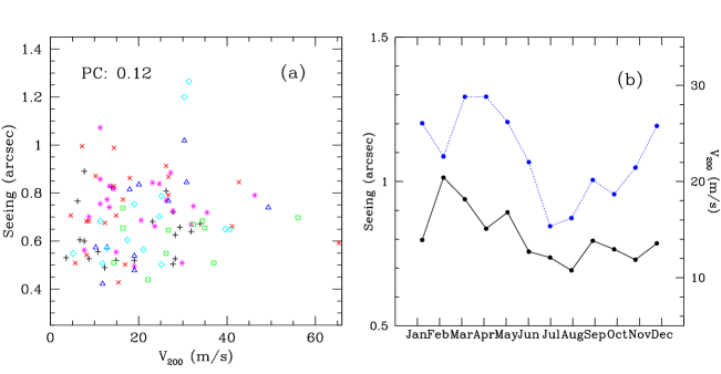
Figure 3: (a) Comparison of seeing and wind speed at 200 mbar pressure level at the OT. The linear Pearson correlation coefficient between both quantities is shown at the top-left. Symbols indicate data from different years: 2003–black crosses; 2004–red Xs; 2005–magenta asterisk; 2006–blue triangles; 2007–cyan rhombus; and 2008–green squares. (b) Seasonal trend of the seeing (black line) and high-altitude winds ($V_{200}$, blue-dashed line) above Roque de los Muchachos Observatory ($\sim 160$ km from the OT and similar altitude above mean sea level, $\sim$2400 m) for the period 1995–2002.

Previous studies have also suggested a possible connection between ground layer wind (speed and direction) to seeing (Chonis, Claver & Sebag 2009; Lombardi et al. 2007; Varela, Muñoz-Tuñón & Gurtubai 2001; Muñoz-Tuñón, Varela & Mahoney 1998; Erasmus 1986). Such a relationship between seeing and $V_{\rm ground}$ seems to be present at OT (Fig. 4(a)) although a large dispersion in the data is clear. In general, larger seeing are obtained as $V_{ground}$ increases. The large dispersion of the data as well as the fact that the best fit derived (seeing=0.56+0.03V_ground) is far from the origin of coordinates could be related to the role played by wind direction. Such dependency of seeing on wind direction has been reported for El Peñón in Chile (Chonis, Claver & Sebag 2009). Looking for an enhancement of this feature, M&E06 studied the correlation between $V_{\rm ground}$ and the ground layer contribution to the seeing in San Pedro Mártir. Figure 4(b) shows the comparision of wind speed at ground level to boundary layer (first km) contribution to the seeing above the OT. A clear correlation between both quantities is present, showing less dispersion than in the seeing–$V_{\rm ground}$ connection. In this case, the interception of the best linear fit, boundary_layer_seeing =0.39+0.04V_ground, is still large, suggesting that another variable (perhaps wind direction) is also playing an important role in the generation of turbulence at the boundary layer.

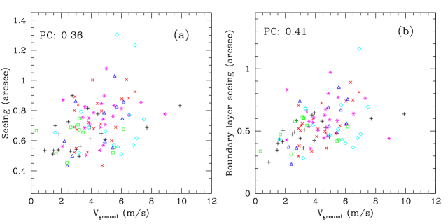
Figure 4: (a) Comparison of seeing and ground level wind speed for the OT. The linear Pearson correlation coefficient between both variables is shown at the top-left. Symbols indicate data from different years: 2003–black crosses; 2004–red Xs; 2005–magenta asterisk; 2006–blue triangles; 2007–cyan rhombus; and 2008–green squares. (b) Comparison of boundary layer (first km) contribution to the seeing and wind speed at ground level at the OT. The linear Pearson correlation coefficient between both quantities is shown at the top-left. Symbols are as in (a).

3.2 Relation between isoplanatic angle and wind speed

A slow trend in the behaviour of the mean isoplanatic angle and $V_{200}$ was reported for Paranal during 2000 (S&T02), although a systematic relation between wind speed and $\theta_{0}$ seems to be non-existant. However, the astroclimatology webpage of the ESO sites (http://www.eso.org/gen-fac/pubs/astclim/paranal/seeing/adaptive-optics/) suggests a connection between $V_{200}$ and isoplanatic angle showing the largest $\theta_{0}$ for the smallest $V_{200}$. At the OT, we do not find any linear relation either with the wind speed at either the 200 mbar level or at ground level and isoplanatic angles obtained from G-SCIDAR profiles (Figure 5). The Pearson correlation coefficients derived comparing night-to-night $\theta_{0}$ with $V_{200}$ and $V_{\rm ground}$ are close to zero, indicating that there are no systematic relations. Unfortunately, we do not have a large enough database of isoplanatic angle measurements at the OT to study any seasonal connection.

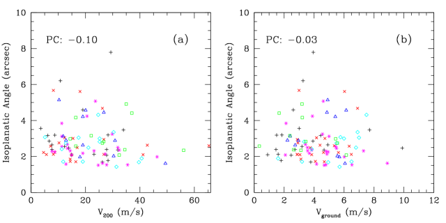
Figure 5: (a) Comparison of isoplanatic angles and 200 mbar pressure level wind speed for the OT. (b) Comparison of isoplanatic angles and wind speed at ground level at the OT. The linear Pearson correlation coefficient between variables is shown at the top-left of each pannel. Symbols indicates data from different years: 2003–black crosses; 2004–red Xs; 2005–magenta asterisk; 2006–blue triangles; 2007–cyan rhombus; and 2008–green squares.

3.3 Average velocity of the turbulence vs. wind speed at 200 mbar

$V_{200}$ was adopted as a parameter for site evaluation mainly thanks to the correlations found at Cerro Pachón (S&T02) and San Pedro Mártir (M&E06) between $V_{0}$ and $V_{200},$ as we already have mentioned. We explore the $V_{0}$–$V_{200}$ connection in detail at the OT with our large dataset. Table 1 presents the best linear fit between $V_{0}$ and $V_{200}$ derived for each year and including all the data.

Table 1: Best linear fit obtained from the average velocity of the turbulence and wind speed at the 200 mbar pressure level measurements for the Teide Observatory. The best fit to the total sample (data from 2003+2004+2005+2006+2007+2008) is labelled “Total”. The last column corresponds to the result when forcing the fit to pass through the coodinate origin (“Best forced linear fit”)

Year	Pearson’s	Best linear fit	Best forced
	coefficient		lineal fit
2003	0.23	7.68+0.07V200	0.44V200
2004	0.74	6.35+0.16V200	0.59V200
2005	0.58	5.34+0.18V200	0.47V200
2006	0.77	3.86+0.23V200	0.45V200
2007	0.70	5.25+0.27V200	0.47V200
2008	0.31	8.21+0.08V200	0.41V200
Total	0.56	6.21+0.16V200	0.47V200

The degree of correlation found at the OT (Table 1) indicates a faint linear relationship between $V_{0}$ and $V_{200}$ during 2003 and 2008, while Pearson’s correlation coefficient for measurements from 2004 to 2007 suggests a clearer linear connection between both quantities. The best linear fit derived from yearly data are far from a linear fit passing through the coordinate origin, as suggested for Paranal/Cerro Pachón (S&T02) and San Pedro Mártir (M&E06). Indeed, we found a relative large $V_{0}$ offset at the coordinate origin that ranges from 3.86 to 8.21 m/s depending on year. In spite of this offset and following the same calculation as S&T02 and M&E06, we have forced the fit to pass through the coordinate origin (Table 1). The proportional factor between $V_{200}$ and $V_{0}$ ranges from 0.41 to 0.59 depending on year (see Table 1), giving a mean value of 0.47$\pm 0.06$. This result indicates how such an approach to estimate $V_{0}$ could induce large errors at the OT.

Combining all the data in the sample (100 measurements), we obtain a Pearson correlation coefficient of 0.56, indicating the degree of linear correlation between V₂₀₀ and $V_{0}$ (Fig. 6(a)). Again, the best linear fit to the total sample presents a large $V_{0}$ offset in the origin (Table 1). The fit forced to pass through the coordinate origin gives 0.47 as the proportionality coefficient, which is in agreement (assuming a dispersion of $\pm 0.06$ in this parameter) with the 0.4$V_{200}$ and 0.56$V_{200}$ found for Cerro/Pachón (S&T02) and San Pedro Mártir (M&E06), respectively.

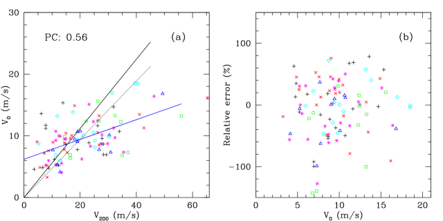
Figure 6: (a) Comparison of the average velocity of the turbulence ($V_{0}$) with wind speed at the 200 mbar pressure level ($V_{200}$) measurements at the OT. The linear Pearson correlation coefficient is shown at the top-left. The black continous line corresponds to $V_{0}=0.56\times V_{200}$ approach found by M&E06 for San Pedro Mártir. The dashed black line indicates the fit forced to pass through the coordinate origin, including the 100 measurements from the sample. The best linear fit to the data ($V_{0}=6.21+0.16V_{200}$) is drawn as a blue line. Symbols indicate data from different years: 2003–black crosses; 2004–red Xs; 2005–magenta asterisk; 2006–blue triangles; 2007–cyan rhombus; and 2008–green squares. (b) Relative error induced by using the linear approach $V_{0}=0.47V_{200}$ at the OT for the full dataset. Negative values indicate smaller estimations of $V_{0}$ than the measured. Symbols are as in (a).

Figure 6(b) presents the relative errors, ($\frac{V_{0}-0.47V_{200}}{V_{0}}$)100%, that we would obtain when estimating $V_{0}$ from $V_{200}$ using the linear factor including all the nights and forcing the fit to pass through the origin derived for OT. Such an approach would induce relative mean errors of $\sim$38%, reaching uncertainties greater than 100% in some cases.

3.3.1 The turbulence characteristic altitude

The characteristic turbulence altitude gives the effective height of the dominant turbulence, increasing when the high-level turbulence dominates. The mean turbulence height can be calculated from:

$$\hat{H}=0.314\frac{r_{0}}{\theta_{0}}$$ (5)

r₀ and $\theta{{}_{0}}$ being the Fried parameter and the isoplanatic angle, respectively (Fried 1976). As both parameters can be derived from G-SCIDAR profiles, the characteristic turbulence altitude can be calculated (see appendix B for daily measurements at OT). The mean $\hat{H}$ derived from the dataset is 3.87$\pm 1.30$ km, suggesting that the turbulence at the OT is distributed in lower-altitude layers than in Paranal or Cerro Pachón, where the average turbulence characteristic altitude was found $\sim 6.4$ km (S&T02).

S&T02 found that measurements providing errors larger than 50% with respect to $V_{0}=0.4\times V_{200}$ correspond to those cases when the characteristic turbulence altitude was smaller than 3 km. From the OT dataset and following the criteria suggested by S&T02, we have selected those data with an equivalent turbulence height larger than 3 km and relative errors smaller than 50% with respect to the $V_{0}$–$V_{200}$ proportionality derived for the OT ($V_{0}=0.47V_{200}$, Fig. 7(a)). Using these cut-offs, the number of selected nights is 56. The Pearson correlation coefficient of $V_{0}$ and $V_{200}$ for this reduced dataset reaches 0.84, giving a proportionality factor of 0.49 when forcing the fit to pass through the coordinate origin. The resulting $V_{200}$ vs. $V_{0}$ diagram (Fig. 7(b)) shows less dispersion in the data, although the best fit of this sub-sample is still far from passing through the origin (best fit: $V_{0}=3.81+0.30V_{200}$).

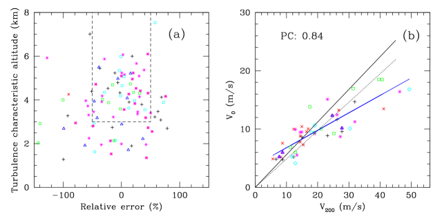
Figure 7: (a) Relative error (%) (when assuming the expression $V_{0}=0.47\times V_{200}$ at the OT) versus the characteristic turbulence altitude. The ashed line marks the region of nights satisfying the selection criteria (see text). (b) Proportionality between $V_{200}$ and $V_{0}$ for selected nights at the OT. The best linear fit to the data ($V_{0}=3.81+0.30V_{200}$) is drawn as a blue line. Symbols indicate data from different years: 2003–black crosses; 2004–red Xs; 2005–magenta asterisk; 2006–blue triangles; 2007–cyan rhombus; and 2008–green squares. The linear Pearson correlation coefficient is shown at the top-left. The black continous line corresponds to $V_{0}=0.56\times V_{200}$ approach found by M&E06 for San Pedro Mártir. The dashed black line indicates the fit forced to pass through the coordinate origin ($V_{0}=0.49V_{200}$) including the selected measurements.

However, for 17% of the nights in the total sample, the relative error respect $V_{0}=0.47V_{200}$ is larger than 50% while the characteristic turbulence altitude is larger than 3 km. Calculating the cumulative $C_{N}^{2}$ distribution, we found that for 15 of these nights, 70% of the turbulence is concentrated under 4 km. For the remaining two nights, more than 50% of the turbulence is in low-altitude layers (under 4 km). We have also noted that for 14 of these 17 nights, the wind vector suffers significant twisters (larger than 50 degrees) from the ground to the 200-mbar level suggesting than wind direction could be influencing any connection.

Therefore, it seems that the linear relationship between $V_{0}$ and $V_{200}$ of the form $V_{0}=A\times V_{200}$ can be adopted only when the characteristic turbulence altitude is larger than around 3 km, as indicated when comparing Figures 6 and Figure 7(b), and when the wind direction might be playing an important role to fix such an approach.

3.4 Average velocity of the turbulence vs. wind speed at ground level

We have selected the data from the total dataset with relative errors larger than 50% respect to the linear relationship $V_{0}=0.47V_{200}$, giving 44 nights. These data are characterized for characteristic turbulence altitudes smaller than 3 km and/or a $C_{N}^{2}$ distribution mainly concentrated under 4 km. We have compared the $V_{0}$ measurement from this subset with the mean wind velocity at ground level during G-SCIDAR observations. $V_{\rm ground}$ data are measured by a weather station placed closer to the Carlos Sánchez Telescope where the G-SCIDAR data are collected. Figure 8(a) shows $V_{0}$ as a function of $V_{\rm ground}$. The Pearson correlation coefficient between $V_{0}$ and $V_{\rm ground}$ is 0.48, the best linear fit being $V_{0}=0.77V_{200}+5.71$. As in section §3.1, we have forced the fit to pass through the coordinate origin, giving $V_{0}=1.74V_{\rm ground}$. Such an approximation would induce mean relative errors (abs($\frac{V_{0}-1.74V_{\rm ground}}{V_{0}}$)100%) of 29%, with a maximum error smaller than 65%. Considering all the nights in the dataset, the slope of the fit passing through the coordinate origin will be 1.80, providing a mean relative error of 41% and a maximum relative error smaller than 100% (see Figure 8(b)). This fact and the results in section §3.2 suggest that $V_{200}$ and $V_{\rm ground}$ could provide estimates of $V_{0}$ with similar (or even bettter) uncertainties.

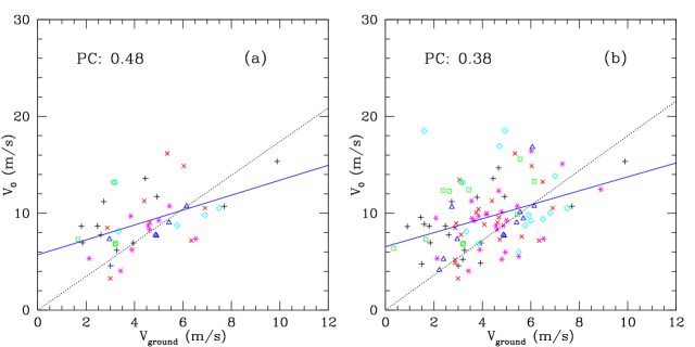
Figure 8: Comparison of the average velocity of the turbulence ($V_{0}$) with wind speed at ground level ($V_{\rm ground}$) measurements at the OT. The linear Pearson correlation coefficient is shown at the top-left: (a) Selected data satisfiying that turbulence are mainly in low-altitude layers (see text). The dashed black line indicates the fit forced to pass through the coordinate origin including the 44 measurements of the sub-sample. The best linear fit to the data is drawn as a blue line; (right) Including all the data (100 nights). The black continous line corresponds to $V_{0}=0.56\times V_{200}$ approach found by M&E06 for San Pedro Mártir. The dashed black line indicates the fit forced to pass through the coordinate origin including the 100 measurements of the sample. The best linear fit to the data is drawn as a blue line ($V_{0}=7.89+0.45*V_{\rm ground}$). Symbols indicates data from different years: (a) 2003: black crosses; (b) 2004: red Xs; (c) 2005: magenta asterisk; (d) 2006: blue triangles; (e) 2007: cyan rhombus; and (f) 2008: green squares.

S&T02 proposed a general formula to estimate $V_{0}$ combining data from ground level and wind speed at 200 mbar pressure level: $V_{0}\simeq$ Max($V_{\rm ground},0.4V_{200}$). According to results in this section and §3.2, such a connection should be of the form $V_{0}\simeq$ Max(1.74$V_{\rm ground},0.49V_{200}$) for the OT. This approach to estimating $V_{0}$ could also induce large errors at the OT, with a mean error of 28%. Large uncertainties and the large intercepts derived for the best fits suggest that wind direction could be playing an important role in these connections.

Unfortunately, any of the relations to estimate $V_{0}$ provide in many cases large errors that are incompatible with the requirements for AO systems. Therefore, the on-site measurement of turbulence and wind profiles is still crucial for optimizing future AO instruments.

3.5 Relation between coherence time and wind speed

A connection between coherence time and wind speed is expected, given that a certain degree of relation exists beween $V_{0}$ and $V_{200}$ or $V_{\rm ground}$. Such a relation is clearly present at San Pedro Mártir (M&E06) and the Chilean sites (S&T02). Figure 9 shows the nightly mean values of $\tau_{0}$ in comparison to wind speeds at the OT. The derived Pearson correlation coefficients indicate a clear inverse connection between $\tau_{0}$ and wind speeds. As a general trend, the larger the wind speed is at ground level, the smaller coherence time obtained. We have fit a curve of the form $\tau_{0}=B$/wind, obtaining $B=20.21$ and $B=95.40$ for $V_{\rm ground}$ and $V_{200}$, respectively.

Previous studies (S&T02; M&E06) actually proposed to estimate $\tau_{0}$ using the proportionality relation $V_{0}=A\times V_{200}$ in Equation 4. We have estimated $\tau_{0}$ through the general approach derived in section §3.4 to estimate $V_{0}$. In this case, mean relative errors smaller than 15% can be obtained, reaching uncertainties smaller than 50% in all the nights in the dataset. According to this result, calculate $\tau_{0}$ from on-site seeing measurements and winds at ground and 200 mbar levels (through the general approach) provide relative good estimates of this AO parameter with acceptable uncertainties.

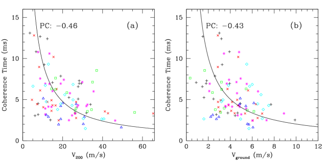
Figure 9: (a) Comparison of the coherence time of the turbulence ($\tau_{0}$) with wind speed at the 200 mbar presseure level ($V_{200}$) for the OT. The black continous line corresponds to the best linear fit: $\tau_{0}=8.35-0.12\times V_{200}$. (b) Comparison of $\tau_{0}$ and wind speed at ground level. The linear Pearson correlation coefficient is shown at the top-left of each pannel. Symbols indicate data from different years: 2003–black crosses; 2004–red Xs; 2005–magenta asterisk; 2006–blue triangles; 2007–cyan rhombus; and 2008–green squares.

4 Discussion

The wind speed at the 200 mbar pressure level has been accepted as an astronomical site evaluation parameter indicative of suitabiblity for adaptive optics. The hypothesis to propose high-altitude winds as a parameter for site evaluation was that the integrated refractive index structure constant is strongly related to the maximum wind speed in the atmosphere that is reached near the 200 mbar pressure level (Vernin 1986). Such a hypothesis seems not to be true at the OT for night-to-night measurements, although a similar seasonal trend between seeing and $V_{200}$ exists as in Mauna Kea and La Silla. Such a hypothesis is not true at the OT in the sense that there are many nights in which the maximum wind speed in the wind vertical profile is far from the 200 mbar presseure level, or even that there does not exist a clear maximum in the profile (see wind vertical profiles in Appendix B). Only 39% of the profiles present a peak at around the 200 mbar pressure level ($\approx 1500$ m above or below the altitude of the 200 mbar level). Wind speed at ground level seems to have more impact on total and boundary layer seeing than $V_{200}$: the larger V_ground is the larger are the seeing values that are expected, although a large dispersion in the measurements is present. Orography and wind direction can have an important influence in increasing such dispersion.

$V_{200}$ as a site evaluation parameter was supported by the empirical results at Cerro Pachón/Paranal (S&T02) and San Pedro Mártir (M&E06), where $V_{0}$ was found to be proportional to $V_{200}$ in the form: $V_{0}=A\times V_{200}$, A being a constant ($A=0.4$ for Cerro Pachón/Paranal; and $A=0.56$ for San Pedro Mártir). Such a relationship is very attractive as it will simplify the problem of knowing the relevant input numbers for AO that could be parameterized in term of $V_{200}$. However, at the Teide Observatory such a relationship seems not to be as smooth as at the Chilean or Mexican sites. Only when the mean altitude of the turbulence is larger than 3 km, $V_{200}$ seems to connect better to $V_{0}$, but even in this case wind direction could have an important influence. We found similar uncertainties when estimating V₀ from $V_{200}$ or $V_{\rm ground}$, suggesting than both wind speeds can be used to simplify the calculation of $V_{0}$ if we are able to assume errors larger than 50% in many cases. In any case, if a gross estimate of $V_{0}$ is required, the use of both wind speeds ($V_{200}$ and $V_{\rm ground}$) can provide better results.

Including the wind speed, other factors (e.g. buoyant convection precesses, inestability phenomena, etc.) may be playing an important role in generating low/medium-altitude turbulence (Stull 1988) that could be breaking the connection with $V_{200}$. Moreover, changes in wind direction or wind regimes (in different seasons, for example) could have an important influence on the linear coefficient connecting $V_{0}$ or seeing with $V_{200}$. Indeed, many of the nights in the sample with large discrepancies with respect to a linear behaviour with V₂₀₀ show significant wind direction gradients from ground to high-altitude levels (see wind direction profiles in Appendix B). The mean wind vector twist from low- to high-altitude levels at the OT (see section §2) and the result could be a break on the influence of high-altitude winds, concentrating the turbulence generators at lower altitudes than in Paranal/Cerro Pachón. Such a twist in wind directions is smoother at the Chilean sites but is more important for the Hawaiian islands (Eff-Darwich et al. 2009). If wind direction changes are really playing an important role, we would expect the faintest night-to-night connection between $V_{0}$ and $V_{200}$ at the Mauna Kea site.

Such a break in the connection between AO parameters and high-altitude winds could be also related with the large variation of the tropopause level above the Canary Islands astronomical sites, ranging from $\sim 200$ to 100 mbar depending on season (García-Lorenzo, Fuensalida & Eff-Darwich 2004). Indeed, during winter and spring the tropopause level could be at a lower-altitude than the 200 mbar pressure level. This means that, depending on season, the 200 mbar pressure level could be in the stratosphere instead of the troposphere at Roque de los Muchachos or Teide Observatories. In contrast, the tropopause level above Paranal or Mauna Kea is always at higher altitudes than the 150 mbar pressure level (García-Lorenzo, Fuensalida & Eff-Darwich 2004).

Despite poor empirical results, the false idea of a connection between image quality and high-altitude wind speed has become increasingly widespread among those in the astronomical community interested in AO. Unfortunately, all of the connections found between winds and AO parameters are relatively faint, and their relations could induce large errors in many cases that are not compatible with the requirements for efficient AO systems. We would like to emphasize the importance of atmospheric on-site turbulence information to evaluate the capabilities of adaptive optics and multi-conjugate adaptive optics systems. Any average or approached value is only a gross estimate of the AO input parameters. If efficient AO is required, the correction system should be prepared for a large variety of turbulence conditions that might be very different from night to night. Therefore, the measurement of turbulence and wind profiles are still crucial for optimizing future instruments with extreme AO capabilities.

In any case, we have demostrated that any factor derived at a site to simplify calculations cannot be easily generalized worldwide but should be obtained for each site. Indeed, the connections between parameters at a particular site might not be valid for any other site due to the pecularities of each location (latitude, longitude, orography, etc.). Any astronomical site evaluator should be checked carefully before any approach is adopted.

5 Summary and Conclusions

We have studied the connection between AO atmospheric parameters and wind speed at the ground and 200 mbar pressure levels by means of a database of 100 nights of G-SCIDAR $C_{N}^{2}$ profiles and balloon data at the Teide Observatory. We have obtained the average profiles ($C_{N}^{2}(h)$ and $V(h)$) above this site and we derived the average seeing, isoplanatic angle and coherence time that confirm the excellent conditions at the OT for AO applications. Our main conclusions can be summarized as follows.

• The connection between night-to-night seeing and wind speed at the 200 mbar pressure level is very faint or non-existent at the OT. However, we found a similar seasonal trend between statistical seeing behaviour and $V_{200}$ that may suggest that $V_{200}$ only plays a secondary role.

• The night-to-night seeing seems to be connected to ground level winds, although a large dispersion is obtained which may be related to the influence of other factors (wind direction, buoyant convection processes, etc.).

• A correlation between wind speed at the site level and the boundary layer contribution to seeing is found. Again, the wind direction could be a factor playing an important role in such a connection.

• The isoplanatic angle is not connected to wind speeds, although a seasonal trend between both variables cannot be roled out.

• The linear connection between the average velocity of the turbulence and wind speed at the 200 mbar pressure level is faint at the OT. Only in those cases where the average altitude of the turbulence is larger than 3 km can a better connection be accepted.

• Similar uncertainties are obtained when estimating $V_{0}$ from winds at ground level or from $V_{200}$. In both cases, the wind direction could play an important role.

• The coherence time presents an inverse linear connection to winds, although it shows a large dispersion.

• Best results are obtained when combining wind speed at ground and the 200 mbar pressure level.

• The large errors derived from any relation between AO parameters and winds are not compatible with the requirements of efficient AO systems. Moreover, such errors could be also a problem when $V_{200}$ is used as a site evaluator.

• The proper characterization of atmospheric turbulence and winds is still crucial for optimizing future instruments with extreme AO capabilities.

The results in this paper indicate that adaptive optics parameters present complex connections to wind speed.

6 APPENDIX A

This appendix includes the average C${}_{N}^{2}$(h) profiles derived from G-SCIDAR measurement from 00UT to 02UT for the 100 nights considered in this work. We also plot the wind speed vertical profile (module and direction) provide by balloons launched from an altitude of 105 meters at about $\sim 13$ km from OT at 00UT.

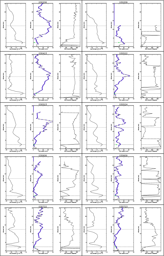
Figure 10: Average C${}_{N}^{2}$ profile and the simultaneous wind vertical profiles (modulus and direction) for the data corresponding to 2003-2008 period at the Teide Observatory. Dates are indicated at the top of each plot. Open squares are the interpolated velocities to the same resolution than turbulence profiles.

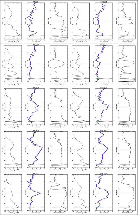
Figure 10: Continuation.

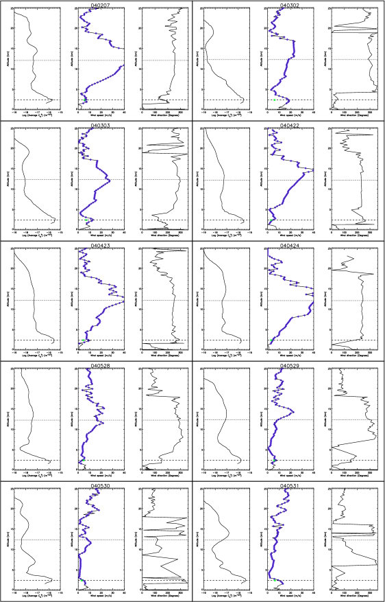
Figure 11: Continuation.

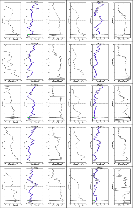
Figure 11: Continuation.

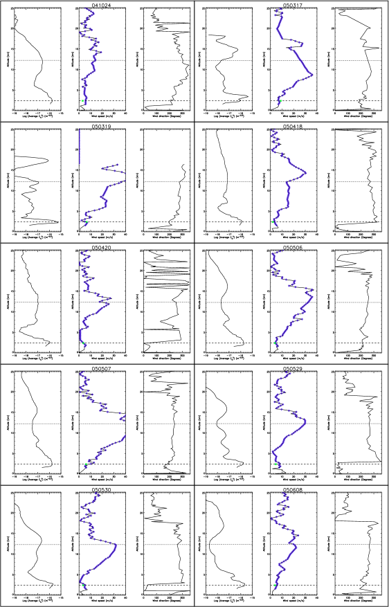
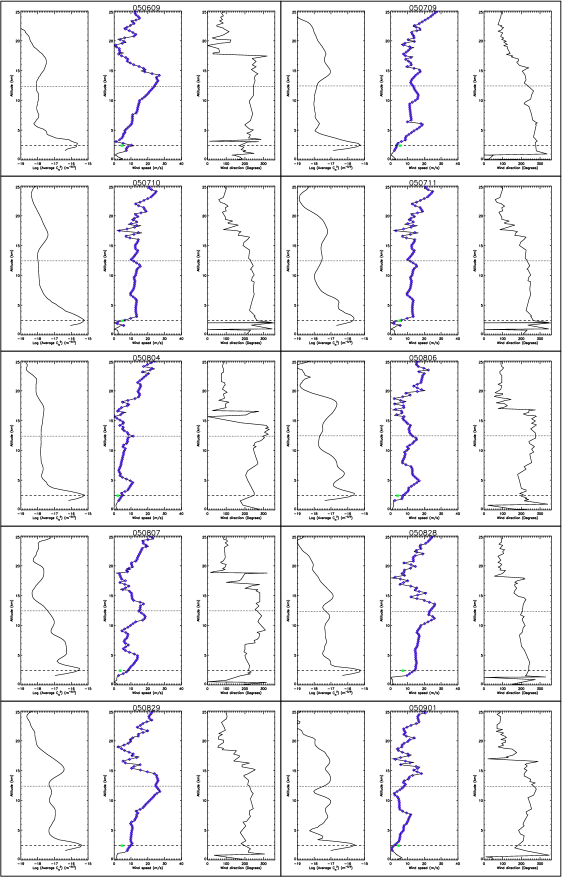
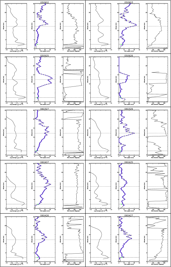
Figure 12: Continuation.

Figure 12: Continuation.

Figure 12: Continuation.

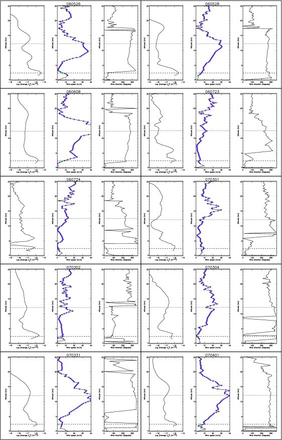
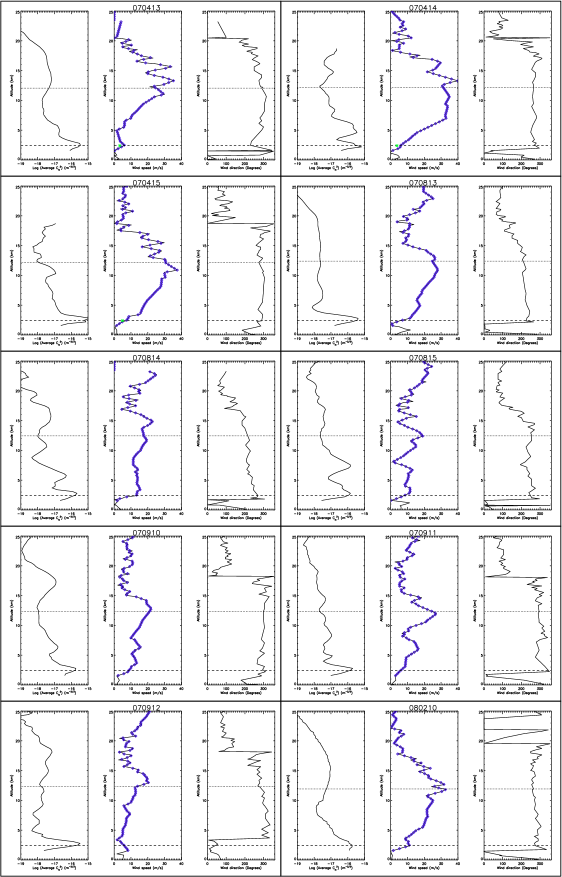
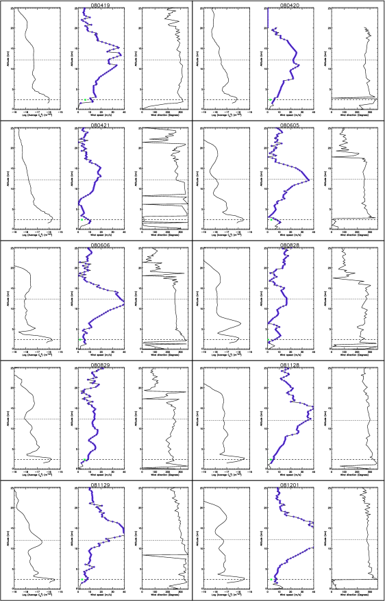
Figure 12: Continuation.

Figure 12: Continuation.

Figure 12: Continuation.

7 APPENDIX B

This appendix includes the dates and wind measurements of 100 nights distributed from 2003 to 2008 used to study the connection of the average velocity of the turbulence and high altitude winds at the Teide observatory. We have also included the number of individual profiles obtained from G-SCIDAR observations approximately during the ballon ascent period used to derive the average C${}_{N}^{2}$ profiles. We also list the computed AO parameters from the C${}_{N}^{2}$(h) and V(h) profiles.

Table 2: Number of individual turbulence profiles from G-SCIDAR measurement used to derived the mean C${}_{N}^{2}$(h) profile corresponding aproximately to the balloon ascent period during 2003, ground level wind (V_ground), wind at the 200 mbar pressure level (V₂₀₀), peak value at the wind vertical profile, and the derived AO parameters (Fried’s parameter, isoplanatic angle, average velocity of the turbulence, coherence time, and turbulence characteristic altitude). The Fried’s parameter and isoplanatic angle correspond to the average value derived from G-SCIDAR measurements during the corresponding balloon ascent and their uncertanties only indicate the standard deviation of the individual values.

Date	Number	Vground	V200	Vmax	r${}_{0}\pm\sigma_{r_{0}}$	$\theta_{0}\pm\sigma_{\theta_{0}}$	V0	$\tau_{0}$	$\hat{H}$
	of profiles	( ms-1 )	( ms-1 )	( ms-1 )	( cm )	( arcsec )	( m/s )	( ms )	( km )
2003-02-06	100	7.700	33.953	37.040	15.032$\pm$2.202	3.476$\pm$1.142	10.710	4.407	2.801
2003-02-09	164	9.889	13.890	22.636	12.274$\pm$1.328	2.468$\pm$0.521	15.346	2.511	3.221
2003-04-23	104	3.950	29.323	35.497	15.373$\pm$3.443	7.793$\pm$5.269	6.935	6.960	1.277
2003-05-22	101	1.458	27.780	32.924	20.067$\pm$2.459	2.388$\pm$0.467	9.571	6.583	5.442
2003-05-23	198	1.603	23.150	46.814	14.826$\pm$2.261	2.121$\pm$0.481	8.869	5.248	4.527
2003-05-24	207	4.921	7.717	23.664	16.860$\pm$1.701	2.650$\pm$0.558	11.705	4.523	4.121
2003-06-06	100	3.264	10.803	18.520	18.201$\pm$2.024	6.212$\pm$2.051	6.175	9.254	1.897
2003-06-09	250	3.009	3.601	17.491	19.061$\pm$2.809	3.559$\pm$0.859	4.569	13.098	3.468
2003-07-22	258	0.900	14.919	27.780	19.443$\pm$3.485	2.099$\pm$0.497	8.626	7.077	5.998
2003-07-23	234	3.194	12.347	24.693	20.683$\pm$2.501	2.560$\pm$0.522	5.235	12.405	5.233
2003-08-04	255	2.731	7.717	26.751	11.350$\pm$1.084	2.386$\pm$0.321	11.202	3.181	3.081
2003-08-05	109	4.444	6.173	30.867	13.189$\pm$1.575	3.167$\pm$0.449	13.595	3.055	2.697
2003-08-06	263	3.924	6.688	29.838	16.704$\pm$1.789	2.855$\pm$0.846	4.844	10.827	3.790
2003-08-07	245	1.500	8.746	27.266	19.188$\pm$2.330	3.186$\pm$0.430	4.753	12.675	3.900
2003-08-28	270	2.611	19.034	27.266	19.428$\pm$2.714	4.589$\pm$1.019	7.760	7.861	2.741
2003-08-29	102	1.806	28.294	31.381	19.208$\pm$3.006	1.774$\pm$0.355	8.661	6.963	7.012
2003-08-30	235	4.667	31.896	34.468	15.794$\pm$1.631	2.363$\pm$0.457	14.679	3.378	4.328
2003-08-31	273	3.778	26.237	29.323	12.507$\pm$1.220	1.690$\pm$0.337	11.642	3.373	4.793
2003-09-13	214	1.852	28.294	30.352	16.157$\pm$2.815	3.195$\pm$0.670	6.950	7.300	3.275
2003-09-15	258	2.472	27.780	31.381	14.027$\pm$1.267	2.070$\pm$0.299	8.675	5.077	4.387

Table 3: Same as table 2 but for 2004.

Date	Number	Vground	V200	Vmax	r${}_{0}\pm\sigma_{r_{0}}$	$\theta_{0}\pm\sigma_{\theta_{0}}$	V0	$\tau_{0}$	$\hat{H}$
	of profiles	( ms-1 )	( ms-1 )	( ms-1 )	( cm )	( arcsec )	( m/s )	( ms )	( km )
2004-02-07	207	5.347	65.334	65.334	17.070$\pm$1.924	2.596$\pm$0.934	16.177	3.313	4.258
2004-03-02	154	6.032	18.006	24.179	11.716$\pm$1.575	5.614$\pm$1.615	14.872	2.473	1.351
2004-03-03	293	6.903	26.237	27.780	11.068$\pm$1.219	4.679$\pm$1.450	10.527	3.301	1.531
2004-04-22	155	2.878	26.751	41.670	12.772$\pm$1.450	2.946$\pm$0.728	8.497	4.719	2.807
2004-04-23	305	4.398	42.699	43.213	11.960$\pm$0.725	2.628$\pm$0.531	11.273	3.331	2.947
2004-04-24	227	3.056	41.156	48.872	15.284$\pm$2.145	2.099$\pm$0.393	13.475	3.561	4.716
2004-05-28	204	4.722	15.433	23.150	23.625$\pm$3.148	3.004$\pm$0.517	7.280	10.189	5.094
2004-05-29	307	5.625	8.746	22.636	14.782$\pm$1.324	2.221$\pm$0.334	7.586	6.118	4.310
2004-05-30	223	2.996	8.231	21.092	18.649$\pm$2.091	5.673$\pm$1.797	3.271	17.902	2.128
2004-05-31	309	6.343	7.202	23.664	10.160$\pm$1.023	2.573$\pm$0.623	7.176	4.444	2.557
2004-07-17	273	3.843	14.919	32.924	14.305$\pm$2.106	2.098$\pm$0.600	10.429	4.307	4.415
2004-07-18	223	6.490	26.751	27.780	11.642$\pm$1.442	2.117$\pm$0.489	13.240	2.761	3.561
2004-08-14	22	4.167	12.347	26.237	14.960$\pm$1.039	3.041$\pm$0.410	9.985	4.704	3.186
2004-08-15	201	2.917	10.289	25.722	11.609$\pm$1.833	2.757$\pm$0.473	8.951	4.072	2.727
2004-08-16	158	3.750	16.977	23.150	20.123$\pm$4.656	2.491$\pm$0.706	10.043	6.291	5.232
2004-09-03	180	2.870	5.659	32.410	19.875$\pm$3.246	2.111$\pm$0.424	4.872	12.809	6.099
2004-09-04	167	2.870	8.231	24.179	14.814$\pm$1.508	2.118$\pm$0.566	5.186	8.968	4.529
2004-09-05	22	4.086	14.404	26.751	10.227$\pm$1.358	1.728$\pm$0.182	8.834	3.635	3.833
2004-09-06	234	4.683	16.462	27.266	13.068$\pm$2.486	1.707$\pm$0.462	9.562	4.291	4.956
2004-10-23	206	4.630	4.630	18.520	14.305$\pm$1.173	2.225$\pm$0.284	9.028	4.975	4.164
2004-10-24	213	3.121	14.404	19.549	12.200$\pm$1.222	1.851$\pm$0.491	7.784	4.921	4.268

Table 4: Same as table 2 but for 2005.

Date	Number	Vground	V200	Vmax	r${}_{0}\pm\sigma_{r_{0}}$	$\theta_{0}\pm\sigma_{\theta_{0}}$	V0	$\tau_{0}$	$\hat{H}$
	of profiles	( ms-1 )	( ms-1 )	( ms-1 )	( cm )	( arcsec )	( m/s )	( ms )	( km )
2005-03-17	38	8.889	26.237	36.526	13.146$\pm$1.378	1.626$\pm$0.197	12.454	3.314	5.236
2005-03-19	41	6.528	35.497	54.531	14.059$\pm$3.931	1.537$\pm$0.243	7.360	5.998	5.923
2005-04-18	82	2.083	14.919	30.867	18.247$\pm$2.233	2.085$\pm$0.197	9.493	6.035	5.668
2005-04-20	55	3.681	19.034	28.294	20.417$\pm$2.512	2.179$\pm$0.237	9.232	6.943	6.067
2005-05-06	338	3.843	32.410	37.554	13.560$\pm$1.104	2.360$\pm$0.454	9.701	4.388	3.722
2005-05-07	349	6.019	46.300	46.814	12.786$\pm$2.018	1.981$\pm$0.275	16.413	2.446	4.180
2005-05-29	314	4.564	29.838	29.838	19.855$\pm$4.514	3.243$\pm$0.559	8.736	7.136	3.964
2005-05-30	307	3.556	31.896	31.896	15.108$\pm$2.309	2.498$\pm$1.019	11.260	4.213	3.916
2005-06-08	242	3.889	20.578	24.179	14.723$\pm$3.359	4.242$\pm$1.592	6.236	7.413	2.248
2005-06-09	241	4.615	23.664	27.266	15.275$\pm$3.688	5.074$\pm$2.139	8.305	5.775	1.949
2005-07-09	48	5.500	13.376	27.780	12.193$\pm$0.879	2.454$\pm$0.231	5.540	6.910	3.217
2005-07-10	293	5.000	11.318	31.381	9.424$\pm$0.710	3.117$\pm$0.656	9.249	3.200	1.957
2005-07-11	336	5.444	11.318	31.381	13.385$\pm$1.275	2.550$\pm$0.478	10.729	3.917	3.399
2005-08-04	111	2.130	11.318	29.838	11.786$\pm$1.395	3.843$\pm$0.861	5.337	6.933	1.986
2005-08-06	357	4.167	12.861	29.838	13.074$\pm$1.638	1.577$\pm$0.301	9.922	4.137	5.369
2005-08-07	346	3.571	14.404	33.439	12.369$\pm$1.192	2.318$\pm$0.576	9.445	4.111	3.455
2005-08-28	206	7.303	23.150	26.751	11.982$\pm$1.303	2.310$\pm$0.366	15.104	2.491	3.358
2005-08-29	251	4.675	24.693	27.266	12.053$\pm$1.282	1.514$\pm$0.296	12.303	3.076	5.156
2005-09-01	146	4.802	7.717	24.179	17.972$\pm$2.087	2.285$\pm$0.380	5.234	10.781	5.093
2005-09-02	275	4.944	8.746	26.237	14.426$\pm$1.416	2.254$\pm$0.531	5.985	7.568	4.145
2005-09-03	195	4.792	27.780	34.468	13.936$\pm$2.054	1.537$\pm$0.363	10.157	4.308	5.870
2005-09-25	323	4.861	27.266	34.468	11.418$\pm$1.347	2.138$\pm$0.488	8.711	4.116	3.459
2005-09-26	323	3.426	13.376	20.578	13.645$\pm$1.911	2.670$\pm$0.506	4.041	10.602	3.309

Table 5: Same as table 2 but for 2006.

Date	Number	Vground	V200	Vmax	r${}_{0}\pm\sigma_{r_{0}}$	$\theta_{0}\pm\sigma_{\theta_{0}}$	V0	$\tau_{0}$	$\hat{H}$
	of profiles	( ms-1 )	( ms-1 )	( ms-1 )	( cm )	( arcsec )	( m/s )	( ms )	( km )
2006-03-27	168	2.738	19.034	28.294	21.165$\pm$4.225	2.629$\pm$0.455	10.637	6.247	5.215
2006-03-29	304	2.963	30.867	31.381	11.968$\pm$1.669	2.883$\pm$0.591	7.320	5.133	2.688
2006-04-07	143	6.146	20.063	31.896	12.097$\pm$1.968	4.569$\pm$1.318	10.733	3.539	1.714
2006-04-25	339	4.907	10.289	15.948	17.625$\pm$2.964	5.140$\pm$1.698	7.679	7.206	2.220
2006-04-26	344	5.417	19.034	24.179	18.785$\pm$2.705	4.210$\pm$1.320	9.022	6.537	2.889
2006-04-27	329	5.694	18.006	25.722	12.409$\pm$1.271	1.968$\pm$0.380	9.441	4.127	4.083
2006-05-26	177	5.556	30.352	36.526	9.927$\pm$0.953	2.023$\pm$0.734	10.105	3.084	3.177
2006-05-28	288	4.861	26.751	30.867	13.183$\pm$1.987	4.449$\pm$1.843	7.761	5.333	1.919
2006-06-08	194	6.065	49.387	50.930	13.671$\pm$0.998	1.611$\pm$0.307	16.817	2.552	5.495
2006-07-23	224	2.222	12.861	26.237	17.603$\pm$3.545	2.897$\pm$0.464	4.136	13.364	3.935
2006-07-24	51	2.400	11.832	30.867	23.963$\pm$3.530	3.121$\pm$0.651	5.263	14.295	4.972

Table 6: Same as table 2 but for 2007.

Date	Number	Vground	V200	Vmax	r0	$\sigma_{r_{0}}\pm\theta_{0}\pm\sigma_{\theta_{0}}$	V0	$\tau_{0}$	$\hat{H}$
	of profiles	( ms-1 )	( ms-1 )	( ms-1 )	( cm )	( arcsec )	( m/s )	( ms )	( km )
2007-03-01	128	5.764	5.144	30.867	18.445$\pm$2.542	3.075$\pm$1.451	8.743	6.624	3.885
2007-03-02	155	3.843	11.318	19.034	14.801$\pm$1.292	2.414$\pm$0.544	6.900	6.734	3.970
2007-03-04	245	3.194	11.832	25.208	19.942$\pm$3.325	1.714$\pm$0.484	13.181	4.750	7.535
2007-03-31	86	1.597	40.641	45.271	15.603$\pm$1.536	1.893$\pm$0.413	18.485	2.650	5.338
2007-04-01	137	4.944	39.612	40.641	15.544$\pm$2.363	1.682$\pm$0.326	18.524	2.635	5.983
2007-04-13	90	3.333	25.208	35.497	12.837$\pm$0.943	2.820$\pm$0.621	8.111	4.969	2.948
2007-04-14	179	5.704	31.381	40.127	7.991$\pm$1.454	1.427$\pm$0.266	16.947	1.481	3.627
2007-04-15	89	6.907	30.352	37.554	8.420$\pm$1.422	3.353$\pm$1.058	9.819	2.693	1.626
2007-08-13	320	7.500	24.693	28.294	14.383$\pm$3.656	4.315$\pm$2.413	10.530	4.289	2.158
2007-08-14	224	7.000	17.491	25.208	16.728$\pm$2.252	3.047$\pm$0.528	13.833	3.797	3.555
2007-08-15	37	6.500	19.034	26.751	13.417$\pm$1.948	1.715$\pm$0.154	9.401	4.481	5.065
2007-09-10	322	6.800	21.092	22.121	17.910$\pm$1.929	2.494$\pm$0.663	10.044	5.599	4.651
2007-09-11	250	6.000	25.208	27.266	20.117$\pm$2.376	2.998$\pm$0.402	9.232	6.842	4.346
2007-09-12	24	5.500	12.861	26.237	17.742$\pm$1.265	2.743$\pm$0.270	5.982	9.312	4.189

Table 7: Same as table 2 but for 2008.

Date	Number	Vground	V200	Vmax	r${}_{0}\pm\sigma_{r_{0}}$	$\theta_{0}\pm\sigma_{\theta_{0}}$	V0	$\tau_{0}$	$\hat{H}$
	of profiles	( ms-1 )	( ms-1 )	( ms-1 )	( cm )	( arcsec )	( m/s )	( ms )	( km )
2008-02-10	58	6.151	32.410	32.924	15.075$\pm$1.295	2.081$\pm$0.354	13.277	3.575	4.691
2008-04-19	171	5.556	26.237	37.040	18.404$\pm$1.671	2.743$\pm$0.372	15.590	3.707	4.345
2008-04-20	188	2.381	22.121	27.266	23.052$\pm$4.316	3.156$\pm$0.446	12.359	5.857	4.731
2008-04-21	50	3.214	16.462	20.063	13.705$\pm$1.630	4.162$\pm$0.859	6.895	6.241	2.132
2008-06-05	265	3.194	34.982	36.011	15.428$\pm$2.558	4.915$\pm$1.562	6.795	7.129	2.033
2008-06-06	97	1.667	37.040	41.156	19.875$\pm$1.899	4.412$\pm$1.039	7.296	8.553	2.917
2008-08-28	310	0.347	16.462	27.266	15.443$\pm$2.180	2.579$\pm$0.518	6.370	7.612	3.878
2008-08-29	329	5.444	14.404	25.722	19.818$\pm$2.726	2.980$\pm$0.566	9.874	6.302	4.307
2008-11-28	75	2.639	34.468	42.699	14.762$\pm$1.186	2.377$\pm$0.377	12.282	3.774	4.022
2008-11-29	313	3.444	26.751	41.670	15.667$\pm$1.866	2.827$\pm$0.659	12.414	3.963	3.588
2008-12-01	89	3.125	56.074	57.618	14.485$\pm$1.632	2.342$\pm$0.395	13.219	3.441	4.005

References

- Avila, Vernin, & Sánchez (2001) Avila, R., Vernin, J., & Sánchez, L.J. 2001, A&A, 369, 364
- Avila et al. (2003) Avila, R., Ibañez, F., Vernin, J., Masciadri, E., Sánchez, L.J., Azouit, M., Agabi, A., Cuevas, S., & Garfias, F. 2003, Rev.Mex.AA, 19, 11
- Bounhir et al. (2008) Bounhir, A., Benkhaldoun, Z., & Sarazin, M. 2008, SPIE, 7016, 66
- Chonis, Claver, & Sebag (2009) Chonis, T.S., Claver, C.F., & Sebag, J. 2009, AAS Meeting, 213, 460.24
- Carrasco, E., Ávila, R., & Carramiñana, A. (2005) Carrasco, E., Ávila, R., & Carramiñana, A. 2005, PASP, 117, 104
- Carrasco & Sarazin (2003) Carrasco, E., & Sarazin, M. 2003, Rev.Mex.AA, 19, 103
- Castro-Almazán, García-Lorenzo, & Fuensalida (2009) Castro-Almazán, J.A., García-Lorenzo, B., & Fuensalida, J.J. 2009, in Optical Turbulence: Astronomy meets Meteorology, eds. E. Masciadri and M. Sarazin-2009
- Chueca et al. (2004) Chueca, S., García-Lorenzo, B., Muñoz-Tuñón, C., & Fuensalida, J.J. 2004, MNRAS, 349, 627
- Eff-Darwich et al. (2009) Eff-Darwich, A., García-Lorenzo, B., Rodríguez-Losada, J.A., de la Nuez, J., Hernández, L.E., & Romero, C. 2009, sent to MNRAS
- Erasmus (1986) Erasmus, D.A. 1986, PASP, 98, 254
- Fried (1976) Fried, D.L. 1976, SPIE, 75, 20
- Fuchs, Tallon, & Vernin (1994) Fuchs, A., Tallon, M., & Vernin, J. 1994, Proc.SPIE,2222,682
- García-Lorenzo et al. 2009 (2009) García-Lorenzo, B., & Fuensalida, J.J., Castro-Almazán, J.A., & Rodríguez-Hernández, M.A.C. 2009, in Optical Turbulence: Astronomy meets Meteorology, eds. E. Masciadri and M. Sarazin-2009
- García-Lorenzo, Fuensalida, & Rodríguez-Hernández (2007) García-Lorenzo, B., Fuensalida, J.J., & Rodríguez-Hernández 2007, SPIE, 674, 11
- García-Lorenzo & Fuensalida (2006) García-Lorenzo, B., & Fuensalida, J.J. 2006, MNRAS, 372, 1483
- García-Lorenzo et al. (2005) García-Lorenzo, B., Fuensalida, J.J., Muñoz-Tuñón, C., & Mendizabal, E. 2005, MNRAS, 356, 849
- García-Lorenzo, Fuensalida & Eff-Darwich (2004) García-Lorenzo, B., Fuensalida, J.J., & Eff-Darwich, A. 2004, SPIE, 5572, 384
- Hardy (1998) Hardy, J.W. 1998, Adaptive Optics for Astronomical Telescopes, by John W Hardy. Foreword by John W Hardy. Oxford University Press
- Ilyasov, S., Tillayev, Y., & Ehgamberdiev, S. (2000) Ilyasov, S., Tillayev, Y., & Ehgamberdiev, S. 2000, SPIE, 4341, 181
- Kluckers et al. (1998) Kluckers, V., Wooder, N., Adcock, M., & Dainty, C. 1998, A&ASuppl.Ser., 130, 141
- Lee, Stull, & Irvine (1984) Lee, D.R., Stull, R.B., & Irvine, W.S. 1984, US Air Force Global Weather Central Technical Note AFGWC/TN 79/001 (revised)
- Lombardi et al. (2007) Lombardi, G., Zitelli, V., Ortolani, S., & Pedani, M. 2007, PASP, 119, 292
- Masciadri & Egner (2006) Masciadri, E., & Egner, S. 2006, PASP, 118, 1604
- Muñoz-Tuñón, Varela & Mahoney (1998) Muñoz-Tuñón, C., Varela, A.M., & Mahoney, T. 1998, NewAR, 42, 409
- Muñoz-Tuñón, Vernin, & Varela (1997) Muñoz-Tuñón, C., Vernin, J. & Varela, A.M. 1997, A&AS, 125, 183
- Prieur et al. (2004) Prieur, J.L., Avila, R., Daigne, G., & Vernin, J. 2004, PASP, 116, 778
- Roddier, Gilli, & Lund (1982) Roddier, F., Gilli, J.J., & Lund, G. 1982, JOpt, 13, 263
- Stull (1988) Stull, R.B. 1988, An introduction to boundary layer meteorology, Atmospheric Sciences Library, Dordrecht: Kluwer
- Varela, Muñoz-Tuñón, & Gurtubai (2001) Varela, A.M., Muñoz-Tuñón, C., & Gurtubai, A.G. 2001, Highlights of Spanish astrophysics II, Proceedings of the 4th Scientific Meeting of the Spanish Astronomical Society (SEA), 301. Dordrecht: Kluwer Academic Publishers, 2001 xxii, 409 p. Edited by Jaime Zamorano, Javier Gorgas, and Jesus Gallego
- Sarazin & Tokovinin (2002) Sarazin M., & Tokovinin A., 2002, in Vernet E., Ragazzoni R., Esposito S., Hubin N., eds, Proc. 58th ESO Conf. Workshop, Beyond Conventional Adaptive Optics. ESO Publications, Garching, 321
- Sarazin (2002) Sarazin M. 2002, ESPAS Site Summary Series: Mauna Kea, Issue 1.1
- Vernin (1986) Vernin, J. 1986, SPIE, 628, 142