Three-dimensional angular momentum projection in relativistic mean-field theory

Abstract

Based on a relativistic mean-field theory with an effective point coupling between the nucleons, three-dimensional angular momentum projection is implemented for the first time to project out states with designed angular momentum from deformed intrinsic states generated by triaxial quadrupole constraints. The same effective parameter set PC-F1 of the effective interaction is used for deriving the mean field and the collective Hamiltonian. Pairing correlations are taken into account by the BCS method using both monopole forces and zero range $\delta$-forces with strength parameters adjusted to experimental even-odd mass differences. The method is applied successfully to the isotopes ²⁴Mg, ³⁰Mg, and ³²Mg.

I Introduction

Experimental and theoretical studies of nuclei far from the $\beta$-stability line are at the forefront of nuclear science. Until 1985 Tanihata85HI , the access to nuclei near the border of $\beta$-stability was practically impossible. The advent of radioactive ion beams (RIBs) Tanihata85PRL ; Bertulani01 provides a useful tool for studying the structure of such unstable nuclei. Hitherto, RIBs have already disclosed many structure phenomena in exotic nuclei with extreme isospin values, and the next generation of radioactive-beam facilities will present new exciting opportunities for the study of the nuclear many-body systems Mueller93 ; Tanihata95 ; Hansen95 ; Casten00 ; Mueller01 ; Jonson04 ; Jensen04 .

Energy density functional (EDF) theory in nuclear physics is nowadays the most important microscopic approach for large-scale nuclear structure calculations in heavy nuclei and it has been successfully employed for the description of nuclei far from $\beta$-stability Bender03 ; Vretenar05 . The nuclear EDF is constructed phenomenologically, based on the knowledge accumulated within modern self-consistent mean-field (SCMF) approaches built upon an effective density-dependent two-body interaction. Compared with the shell model approach Otsuka01 ; CMZ.05 , EDF functionals are universal in the sense that they can be applied to nuclei all over the periodic table. Because of its simplicity SCMF approaches have a great advantage in particular for the description of heavy exotic nuclei.

The great success achieved by SCMF theories in the description of nuclear properties relies on the fact that within these theories the complicated many-body wave functions are approximated by a single Slater determinant. Important many-body correlations are taken into account via the mechanism of “spontaneous symmetry breaking” Ring80 . Examples are the violation of SO(3) rotational symmetry in deformed nuclei and of U(1) symmetry in gauge space in superfluid nuclei. As a consequence, such product wave functions are not eigenstates of the angular momentum and particle number operators. These deficiencies give rise to several serious problems in the description of particular nuclear properties, as the absence of correlations associated with the symmetry restoration, the admixture of low-lying excited states into the ground state, difficulties in the connection to the laboratory frame for spectroscopic observables, the absence of selection rules for transitions, etc. Therefore, in order to compare properly with the experimental data, one has to go beyond the mean-field approximation. Projection methods provide an effective tool to restore the spontaneous breaking of symmetries Yoc.57 ; PY.57 ; Zeh.65 ; MacDonald70 ; Wong75 . A suitable linear combination of intrinsic states deformed in Euler space or gauge space recover rotational or gauge symmetry. Such procedures are known as Angular Momentum Projection (AMP) or Particle Number Projection (PNP) methods.

Angular Momentum Projection has been a goal of nuclear physicists for many years. However, due to its numerical complexity, only in the last ten years it has been possible to apply such projection procedure in the context of SCMF theory with realistic effective forces, for example the non-relativistic Skyrme force SLy4 Valor00 , the Gogny force D1S RER.02a ; Guzman02npa or the relativistic point coupling force PC-F1 Niksic06I ; Niksic06II . These investigations have shown that the energy gain due to the restoration of rotational symmetry is of the order of several MeV and it has great influence on the topological structure of the nuclear potential energy surface (PES). In these three cases, however, axial symmetry in the mean-fields has been imposed from the beginning. Such a restriction simplifies the numerical problem considerably, because in this case, the integrals over two of the three Euler angles in the kernels can be treated analytically and one is left with a one-dimensional integration.

As illustrated by recent systematic calculations Moller06 , specific combinations of single-particle orbitals near the Fermi surface and the additional binding energy due to non-axial degrees of freedom can enhance the tendency to form nuclei with triaxial shapes. Several islands of triaxiality have been revealed throughout the nuclear chart. The inclusion of triaxiality can dramatically reduce the barrier separating prolate and oblate minima, leading to structures that are soft or unstable for triaxial distortions Cwiok05 . Furthermore, the occurrence of triaxiality can give rise to many very interesting modes of collective motion, which are very different from those of axially deformed shape, such as Chiral rotation Grodner06 , Wobbling motion Odegard01 and the violation of $K$-selection rules in electromagnetic transitions Chowdhury88 .

To describe properly the properties of possible triaxially deformed nuclei and especially to examine the role of triaxial deformation in the context of SCMF theory, it is essential to introduce the $\gamma$-degree of freedom at the mean-field level and to perform full three-dimensional angular momentum projection (3DAMP). In the context of phenomenological models with small shell model spaces and the corresponding effective interactions, 3DAMP has already been implemented many years ago in Refs. Giraud69 ; Hara82 ; Hayashi84 ; Burzynski95 ; Enami99 . The restoration of rotational symmetry has been shown to have a strong influence on the topological structure of the ($\beta,\gamma$) energy surface for transitional nuclei Hayashi84 . In particular, the correlations taken into account by 3DAMP are found to have a tendency to lower the potential energy in the region of strong triaxial deformations Enami00ptp . In the context of energy density functionals, 3DAMP has been performed on top of Hartree-Fock (HF) with a simple Skyrme-type interaction Baye84 , or with the full Skyrme energy functional Zdunczuk07 . In both cases cranked wave functions were projected to approximate a variation after projection procedure, but pairing correlations were not included. Only very recently, 3DAMP+PNP with configuration mixing has been attempted in the context of triaxial Hartree-Fock-Bogoliubov (HFB) theory with the full Skyrme energy functional Bender08 .

During the past decades, relativistic mean-field (RMF) theory, which relies on basic ideas of effective field theory LNP.641 and of density functional theory KS.65 has achieved great success in describing many nuclear phenomena for both stable and exotic nuclei over the entire nuclear chart with a few universal parameters Serot86 ; Reinhard89 ; Ring96 ; Vretenar05 ; Meng06 . It incorporates many important relativistic effects, such as the presence of large Lorentz scalar and vector fields with approximately equal magnitude and opposite sign. This leads to a new saturation mechanism via the difference between the scalar and vector densities, and naturally to the large spin-orbit splitting needed for the understanding of magic numbers in finite nuclei. Moreover, relativistic effects are responsible for the efficient description of spin observables in medium-energy proton-nucleus scattering using the relativistic impulse approximation Murdock86 and for the existence of approximate pseudospin symmetry in nuclear spectra Arima69 ; Ginocchio97 . All these features motivate further investigations in the framework of RMF theory and new efforts to improve its predictive power.

The extension of RMF theory for the description of triaxially deformed nuclei was first done decades ago Koepf88 . Later it has been employed in many studies on the effect of $\gamma$ deformation on nuclear properties Hirata96 ; Bender98 ; Meng06prc ; Yao08 . $\gamma$-deformation plays also an important role in the mean field description of rotating nuclei in the framework of the cranking model Koepf89 : the Coriolis operator violates axial symmetry and leads to currents and time-odd components in the intrinsic nuclear fields Afanasjev00b . All these applications of triaxial RMF theory are done on the mean field level. A full 3DAMP for such cases is still missing and strongly desired, especially for the description of transitional nuclei. In this work, we apply for the first time 3DAMP to restore rotational symmetry for triaxially deformed intrinsic states in the framework of RMF theory based on point coupling interactions.

The paper has been arranged as follows. In Sec. II we present an outline of the relativistic point coupling model that will be used to generate mean-field wave functions with triaxial symmetry, and we discuss three-dimensional angular momentum projection. The method is applied for several isotopes, ²⁴Mg, ³⁰Mg, and ³²Mg to check the numerical accuracy of the code as well as to present several illustrative results in Sec. III. Finally, a summary and a perspective is given in Sec. IV. Formulae of 3DAMP, and details about the calculations of contractions and overlaps in the relativistic case are collected in the Appendix.

II Framework

II.1 The relativistic mean-field theory with point coupling

A detailed description of RMF theory with point coupling that will be adopted to generate intrinsic wave functions can be found in Ref. Burvenich02 . In order to present a self-contained description of our approach we will give here a short outline of the relativistic point coupling model used in our applications.

The elementary building blocks of a RMF theory with point coupling vertices are

$$(\bar{\psi}{\cal O}\Gamma\psi),\quad{\cal O}\in\{1,\vec{\tau}\},\quad\Gamma\in\{1,\gamma_{\mu},\gamma_{5},\gamma_{5}\gamma_{\mu},\sigma_{\mu\nu}\},$$ (1)

where $\psi$ is the Dirac spinor field of nucleon, $\vec{\tau}$ is the isospin vector and $\Gamma$ is one of the $4\times 4$ Dirac matrices. There are ten such building blocks characterized by their transformation characteristics in isospin and in Minkowski space. We adopt arrows to indicate vectors in isospin space and bold types for the space vectors. Greek indices $\mu$ and $\nu$ run over the Minkowski indices 0, 1, 2, 3.

A general effective Lagrangian can be written as a power series in $\bar{\psi}{\cal O}\Gamma\psi$ and their derivatives. In present work, we start with the following Lagrangian density:

$${\cal L}={\cal L}^{\rm free}+{\cal L}^{\rm 4f}+{\cal L}^{\rm hot}+{\cal L}^{\rm der}+{\cal L}^{\rm em},$$ (2)

where the Lagrangian density for free nucleon reads

$${\cal L}^{\rm free}=\bar{\psi}(i\gamma_{\mu}\partial^{\mu}-m)\psi.$$ (3)

The four-fermion point coupling term is given by

$${\cal L}^{\rm 4f} = -\frac{1}{2}\alpha_{S}(\bar{\psi}\psi)(\bar{\psi}\psi)-\frac{1}{2}\alpha_{TS}(\bar{\psi}\vec{\tau}\psi)\cdot(\bar{\psi}\vec{\tau}\psi)$$ (4)

$$-\frac{1}{2}\alpha_{V}(\bar{\psi}\gamma_{\mu}\psi)(\bar{\psi}\gamma^{\mu}\psi)$$

$$-\frac{1}{2}\alpha_{TV}(\bar{\psi}\vec{\tau}\gamma_{\mu}\psi)\cdot(\bar{\psi}\vec{\tau}\gamma^{\mu}\psi),$$

which contains scalar-isoscalar, scalar-isovector, vector-isoscalar and vector-isovector channels. The medium dependence of the effective interaction has been taken into account by the higher order interaction terms

$${\cal L}^{\rm hot}=-\frac{1}{3}\beta_{S}(\bar{\psi}\psi)^{3}-\frac{1}{4}\gamma_{S}(\bar{\psi}\psi)^{4}-\frac{1}{4}\gamma_{V}[(\bar{\psi}\gamma_{\mu}\psi)(\bar{\psi}\gamma^{\mu}\psi)]^{2},$$ (5)

As in the nonrelativistic Skyrme functional VB.72 gradient terms are essential. They simulate to some extent the effect of finite range of the force:

$${\cal L}^{\rm der} = -\frac{1}{2}\delta_{S}\partial_{\nu}(\bar{\psi}\psi)\partial^{\nu}(\bar{\psi}\psi)-\frac{1}{2}\delta_{TS}\partial_{\nu}(\bar{\psi}\vec{\tau}\psi)\cdot\partial^{\nu}(\bar{\psi}\vec{\tau}\psi)$$ (6)

$$-\frac{1}{2}\delta_{V}\partial_{\nu}(\bar{\psi}\gamma_{\mu}\psi)\partial^{\nu}(\bar{\psi}\gamma^{\mu}\psi)$$

$$-\frac{1}{2}\delta_{TV}\partial_{\nu}(\bar{\psi}\vec{\tau}\gamma_{\mu}\psi)\cdot\partial^{\nu}(\bar{\psi}\vec{\tau}\gamma^{\mu}\psi).$$

In principle, one could construct many more higher order interaction terms, or derivative terms of higher order, but in practice only a relatively small set of free parameters can be adjusted from the data of ground-state nuclear properties. The electromagnetic interaction between protons is described as usual

$${\cal L}^{\rm em}=-\frac{1}{4}F^{\mu\nu}F_{\mu\nu}-e\bar{\psi}\gamma^{\mu}\dfrac{1-\tau_{3}}{2}\psi A_{\mu},$$ (7)

where $e$ is the charge unit for protons and it vanishes for neutrons. The total Lagrangian density (2) contains eleven coupling constants $\alpha_{S}$, $\alpha_{V}$, $\alpha_{TV}$, $\alpha_{TS}$, $\beta_{S}$, $\gamma_{S}$, $\gamma_{V}$, $\delta_{S}$, $\delta_{V}$, $\delta_{TS}$ and $\delta_{TV}$. The subscripts indicate the symmetry of the couplings: $S$ stands for scalar, $V$ for vector, and $T$ for isovector, while the symbol refer to the additional distinctions: $\alpha$ refers to four-fermion term, $\delta$ to derivative couplings, and $\beta$ and $\gamma$ to the third- and fourth-order terms, respectively.

The pseudoscalar $\gamma_{5}$ and pseudovector $\gamma_{5}\gamma_{\mu}$ channels do not contribute at the Hartree level due to the parity conservation in nuclei and therefore we have neglected it in the Lagrangian density (2). From the experience of RMF with finite-range (RMF-FR) meson exchange, a fit, which includes the isovector-scalar interaction has not been found to improve the description of nuclear ground state observables. This part of the interaction is therefore neglected. Consequently, there are nine free parameters in RMF-PC model, which is comparable with those in RMF-FR model.

Using the mean-field approximation and the “no-sea” approximation, the operators $\bar{\psi}(\hat{\cal O}\Gamma)_{i}\psi$ in Eq. (2) are replaced by their expectation values and become bilinear forms of the Dirac spinor $\psi_{k}$ for nucleons

$$\bar{\psi}(\hat{\cal O}\Gamma)_{i}\psi\rightarrow\langle\Phi|\bar{\psi}(\hat{\cal O}\Gamma)_{i}\psi|\Phi\rangle=\sum_{k}v^{2}_{k}\bar{\psi}_{k}(\hat{\cal O}\Gamma)_{i}\psi_{k},$$ (8)

where $i$ indicates $S,V$, and $TV$. The sum $\sum\limits_{k}$ runs over only positive-energy states with the occupation probabilities $v^{2}_{k}$. Based on these assumptions, one finds the energy density functional for a nuclear system:

$$E_{\rm DF}[\mbox{\boldmath$\tau$},\rho_{S},j^{\mu}_{i},A_{\mu}]=\int d^{3}r~{}{\mathcal{E}(\bm{r}}),$$ (9)

where the energy density

$$\mathcal{E}(\bm{r})=\mathcal{E}^{\rm kin}(\bm{r})+\mathcal{E}^{\rm int}(\bm{r})+\mathcal{E}^{\rm em}(\bm{r})$$ (10)

has a kinetic part

$$\mathcal{E}^{\rm kin}(\bm{r})=\tau(\bm{r})=\sum_{k}\,v_{k}^{2}~{}{\psi^{\dagger}_{k}(\bm{r})\left(\bm{\alpha}\bm{p}+\beta m-m\right)\psi_{k}(\bm{r})},$$ (11)

an interaction part

$$\mathcal{E}^{\rm int}(\bm{r}) = \frac{\alpha_{S}}{2}\rho_{S}^{2}+\frac{\beta_{S}}{3}\rho_{S}^{3}+\frac{\gamma_{S}}{4}\rho_{S}^{4}+\frac{\delta_{S}}{2}\rho_{S}\triangle\rho_{S}$$

$$+\frac{\alpha_{V}}{2}j_{\mu}j^{\mu}+\frac{\gamma_{V}}{4}(j_{\mu}j^{\mu})^{2}+\frac{\delta_{V}}{2}j_{\mu}\triangle j^{\mu}$$

$$+\frac{\alpha_{TV}}{2}\vec{j}^{\mu}_{TV}\cdot(\vec{j}_{TV})_{\mu}+\frac{\delta_{TV}}{2}\vec{j}^{\mu}_{TV}\cdot\triangle(\vec{j}_{TV})_{\mu},$$

which contains the local densities and currents

$$\rho_{S}(\bm{r}) = \sum_{k}v^{2}_{k}\bar{\psi}_{k}(\bm{r})\psi_{k}(\bm{r}),$$ (13a)

$$j^{\mu}_{V}(\bm{r}) = \sum_{k}v^{2}_{k}\bar{\psi}_{k}(\bm{r})\gamma^{\mu}\psi_{k}(\bm{r}),$$ (13b)

$$\vec{j}^{\mu}_{TV}(\bm{r}) = \sum_{k}v^{2}_{k}\bar{\psi}_{k}(\bm{r})\vec{\tau}\gamma^{\mu}\psi_{k}(\bm{r}).$$ (13c)

and an electromagnetic part

$$\mathcal{E}^{\rm em}(\bm{r})=\frac{1}{4}F_{\mu\nu}F^{\mu\nu}-F^{0\mu}\partial_{0}A_{\mu}+eA_{\mu}j^{\mu}_{p}.$$ (14)

Minimization of the energy density functional (9) with respect to $\bar{\psi}_{k}$ gives rise to the Dirac equation (i.e., Kohn-Sham equation) for the single nucleons

$$[\gamma_{\mu}(i\partial^{\mu}-V^{\mu})-(m+S)]\psi_{k}=0.$$ (15)

The single-particle effective Hamiltonian contains local scalar $S(\bm{r})$ and vector $V^{\mu}(\bm{r})$ potentials

$$S(\bm{r})=\Sigma_{S},\quad V^{\mu}(\bm{r})=\Sigma^{\mu}+\vec{\tau}\cdot\vec{\Sigma}^{\mu}_{TV},$$ (16)

where the nucleon scalar-isoscalar $\Sigma_{S}$, vector-isoscalar $\Sigma^{\mu}$ and vector-isovector $\vec{\Sigma}^{\mu}_{TV}$ self-energies are given in terms of the various densities

$$\Sigma_{S} = \alpha_{S}\rho_{S}+\beta_{S}\rho^{2}_{S}+\gamma_{S}\rho^{3}_{S}+\delta_{S}\triangle\rho_{S},$$ (17a)

$$\Sigma^{\mu} = \alpha_{V}j^{\mu}_{V}+\gamma_{V}(j^{\mu}_{V})^{3}+\delta_{V}\triangle j^{\mu}_{V}+eA^{\mu},$$ (17b)

$$\vec{\Sigma}^{\mu}_{TV} = \alpha_{TV}\vec{j}^{\mu}_{TV}+\delta_{TV}\triangle\vec{j}^{\mu}_{TV}.$$ (17c)

For ground state of an even-even nucleus one has time reversal symmetry and the space-like components of the currents ${\mathbf{j}}_{i}$ in Eq. (13) and the spatial part of the vector potential ${\mathbf{V}}(\bm{r})$ in Eq. (16) vanish. Moreover, because of charge conservation in nuclei, only the 3rd-component of isovector potentials $\vec{\Sigma}^{\mu}_{TV}$ contributes. The Coulomb field $A_{0}$ is determined by Poisson’s equation.

In addition to the self-consistent mean-field potentials, for open-shell nuclei, pairing correlations are taken into account by the BCS method with a smooth cutoff factor $f_{k}$ to simulate the effects of finite-range Krieger90 ; Bender00p , i.e. we have to add to the functional (9) a pairing energy depending on the pairing tensor $\kappa$ of the form

$$E_{\rm pair}[\kappa,\kappa^{*}]=\sum_{kk^{\prime}>0}f_{k}f_{k^{\prime}}\langle k{\bar{k}}|V^{pp}|k^{\prime}{\bar{k}}^{\prime}\rangle\kappa^{\ast}_{k}\kappa_{k^{\prime}}.$$ (18)

with the smooth cut-off weight factors

$$f_{k}=\frac{1}{1+\exp[(\epsilon_{k}-\epsilon_{F}-\Delta E_{\tau})/\mu_{\tau}]},$$ (19)

where $\epsilon_{k}$ is the eigenvalue of the self-consistent single-particle field. $\epsilon_{F}$ is the chemical potential determined through the constraint on average particle number: $\langle\Phi|\hat{N}_{\tau}|\Phi\rangle=N_{\tau}$. The cut-off parameters $\Delta E_{\tau}$ and $\mu_{\tau}=\Delta E_{\tau}/10$ are chosen in such a way that $2\displaystyle\sum_{k>0}f_{k}=N_{\tau}+1.65N^{2/3}_{\tau}$, where $N_{\tau}$ is the particle number of neutron or proton.

In the following calculations we use both a monopole force and a density-independent $\delta$-force in the pairing channel respectively. In the case of the monopole force we have $\kappa_{k}=u_{k}v_{k}$ and

$$E_{\rm pair}[\kappa,\kappa^{*}]=-\sum_{\tau=n,p}G_{\tau}\left|\sum_{k>0}f_{k}u_{k}v_{k}\right|^{2}.$$ (20)

In the case of a $\delta$-force we use

$$E_{\rm pair}[\kappa,\kappa^{*}]=-\sum_{\tau=n,p}\dfrac{V_{\tau}}{4}\int d^{3}r\kappa^{\ast}_{\tau}(\bm{r})\kappa_{\tau}(\bm{r}).$$ (21)

where $V_{\tau}$ is the constant pairing strength and the pairing tensor $\kappa(\bm{r})$ is given by

$$\kappa(\bm{r})=-2\sum_{k>0}f_{k}u_{k}v_{k}|\psi_{k}(\bm{r})|^{2}.$$ (22)

The pairing strength parameters $G_{\tau}$ in the case of monopole pairing and $V_{\tau}$ for zero range pairing forces are adjusted by fitting the average single-particle pairing gap

$$\langle\Delta\rangle\equiv\frac{\sum_{k}f_{k}v_{k}^{2}\Delta_{k}}{\sum_{k}f_{k}v_{k}^{2}}$$ (23)

to the experimental odd-even mass difference obtained with a five-point formula.

Moreover, the proper treatment of center of mass (c.m.) motion has been found very important in the binding energy of light nuclei Bender00c ; Long04 ; Chen07 . We adopt the same c.m. correction to the total energy after variation, as it has been used in adjusting the parameter set PC-F1 Bender00c ,

$$E^{\rm mic}_{\rm cm}=-\displaystyle\frac{1}{2mA}\langle\hat{\mathbf{P}}^{2}_{\rm cm}\rangle,$$ (24)

where $m$ is the mass of neutron or proton. $A$ is mass number and $\hat{\mathbf{P}}_{\rm cm}=\sum_{i}^{A}\hat{\mathbf{p}}_{i}$ is the total momentum in the c.m. frame.

The total energy for the nuclear system becomes

$$E_{\rm tot.}=E_{\rm DF}[\mbox{\boldmath$\tau$},\rho_{S},j^{\mu}_{i},A_{\mu}]+E_{\rm pair}[\kappa,\kappa^{*}]+E^{\rm mic}_{\rm cm}.$$ (25)

To obtain the potential energy surface (PES), the mass quadrupole moment is constrained through the quantities $q_{20}$ and $q_{22}$, which are related to the triaxial deformation parameters $\beta$ and $\gamma$ of the Bohr Hamiltonian by

$$q_{20} = \sqrt{\frac{5}{16\pi}}\langle 2z^{2}-x^{2}-y^{2}\rangle=\frac{3}{4\pi}AR^{2}_{0}\beta\cos\gamma,~{}~{}~{}~{}~{}~{}~{}~{}~{}~{}~{}$$ (26a)

$$q_{22} = \sqrt{\frac{15}{32\pi}}\langle x^{2}-y^{2}\rangle=\frac{3}{4\pi}AR^{2}_{0}\frac{1}{\sqrt{2}}\beta\sin\gamma,$$ (26b)

where $R_{0}=1.2A^{1/3}$ fm. The total mass quadrupole moment $q$ is thus given by

$$q=\sqrt{\frac{16\pi}{5}}\sqrt{q^{2}_{20}+2q^{2}_{22}}.$$ (27)

We thus obtain mean field wave functions $|\Phi(\beta,\gamma)\rangle$ that depend on the deformation parameters $\beta$ and $\gamma$. In the following we abbreviate the pair of deformation parameters by a single letter $q=(\beta,\gamma)$.

II.2 Three dimensional angular momentum projection

The nuclear mean-field wave function $|\Phi\rangle$ is a product of the solutions of the deformed Dirac equation of Eq. (15) and therefore it does not have good angular momentum. To obtain the collective energy spectrum and wave functions with the good angular momentum $J$, it is crucial to restore the spontaneously broken rotational symmetry. Especially, for triaxially deformed states $|\Phi(q)\rangle$ with the deformation parameters $q=(\beta,\gamma)$, a full 3DAMP is required.

The wave function $|\Psi^{JM}_{\alpha,q}\rangle$ in the laboratory frame, that is an eigenfunction of $\hat{J}^{2}$ and $\hat{J}_{z}$ with the eigenvalues $J(J+1)$ and $M$, is obtained by projection Ring80

$$|\Psi^{JM}_{\alpha,q}\rangle=\sum_{K}f^{JK}_{\alpha}(q)|JMK,q\rangle,$$ (28)

where $\alpha=1,2,\cdots$ labels the different collective excited states. The basis $|JMK,q\rangle$ functions are not just simply Wigner $D$-functions as adopted in the classical triaxial rotor model but they are determined microscopically from the intrinsic state $|\Phi(q)\rangle$ by projection using the operators $\hat{P}^{J}_{MK}$

$$|JMK,q\rangle=\hat{P}^{J}_{MK}|\Phi(q)\rangle.$$ (29)

The projector-like operator $\hat{P}^{J}_{MK}$ has the form,

$$\hat{P}^{J}_{MK}=\frac{2J+1}{8\pi^{2}}\int d\Omega D^{J\ast}_{MK}(\Omega)\hat{R}(\Omega),$$ (30)

with $\Omega$ representing a set of the three Euler angles ($\phi,\theta,\psi$) and the measure $d\Omega=d\phi\sin\theta d\theta d\psi$. $D^{J}_{MK}(\Omega)$ is the Wigner $D$-function with the rotational operator chosen in the notation of Edmonds Edmonds57 as $\hat{R}(\Omega)=e^{i\phi\hat{J}_{z}}e^{i\theta\hat{J}_{y}}e^{i\psi\hat{J}_{z}}$. The effect of $\hat{P}^{J}_{MK}$ is extracting from the intrinsic state $|\Phi(q)\rangle$ the component with an eigenvalue $K$ of the angular momentum projection along the intrinsic $z$-axis Corbett71 ; Ring80 . Since $K$ is not a good quantum number for a triaxial shape, all these components must be mixed, which corresponds to the so-called “K-mixing”. Considering the $D_{2}$ symmetry of triaxial shape for even-even nuclei, the sum in Eq. (28) is restricted to non-negative even values of $K$. The wave function $|\Psi^{JM}_{\alpha,q}\rangle$ is therefore simplified as Ring80 ; Burzynski95

$$|\Psi^{JM}_{\alpha,q}\rangle=\sum_{K\geq 0}\frac{f^{JK}_{\alpha}(q)}{1+\delta_{K0}}|JMK+,q\rangle,$$ (31)

where the angular momentum projected $K$-component, $|JMK+,q\rangle$, is given by

$$|JMK+,q\rangle=[\hat{P}^{J}_{MK}+(-1)^{J}\hat{P}^{J}_{M-K}]|\Phi(q)\rangle.$$ (32)

The expansion coefficients $f^{JK}_{\alpha}(q)$ are determined requiring that the energy evaluated on $|\Psi^{JM}_{\alpha,q}\rangle$ is stationary with respect to $f^{JK\ast}_{\alpha}(q)$. This condition leads to the generalized eigenvalue equation

$$\sum_{K^{\prime}\geq 0}\{{\cal H}^{J}_{KK^{\prime}}(q;q)-E^{J}_{\alpha}{\cal N}^{J}_{KK^{\prime}}(q;q)\}f^{JK^{\prime}}_{\alpha}(q)=0,$$ (33)

where the overlap kernels ${\cal O}^{J}_{KK^{\prime}}(q;q)$ are determined by (${\cal O}={\cal N},{\cal H}$):

$${\cal O}^{J}_{KK^{\prime}}(q;q) = \Delta_{KK^{\prime}}[O^{J}_{KK^{\prime}}(q;q)+(-1)^{2J}O^{J}_{-K-K^{\prime}}(q;q)$$

$$+(-1)^{J}O^{J}_{K-K^{\prime}}(q;q)+(-1)^{J}O^{J}_{-KK^{\prime}}(q;q)],$$

with $\hat{O}=1,\hat{H}$, and $\Delta_{KK^{\prime}}=1/[(1+\delta_{K0})(1+\delta_{K^{\prime}0})]$

$$O^{J}_{KK^{\prime}}(q;q)=\frac{2J+1}{8\pi^{2}}\int d\Omega D^{J\ast}_{KK^{\prime}}\langle\Phi(q)|\hat{O}\hat{R}|\Phi(q)\rangle.$$ (35)

The details about the calculation of overlap functions $\langle\Phi(q)|\hat{O}\hat{R}(\Omega)|\Phi(q)\rangle$ will be given in the next section.

The generalized eigenvalue equation (33) is solved in the standard way as discussed in Ref. Ring80 . It is accomplished by diagonalizing the norm kernel ${\cal N}^{J}_{KK^{\prime}}(q;q)$ first

$$\sum_{K^{\prime}\geq 0}{\cal N}^{J}_{KK^{\prime}}(q;q)u^{JK^{\prime}}_{m}(q)=n^{J}_{m}u^{JK}_{m}(q).$$ (36)

The eigenfunctions $u^{JK}_{m}(q)$ form a complete orthonormalized set

$$\sum_{m}u^{\ast JK}_{m}(q)u^{JK^{\prime}}_{m}(q)=\delta_{KK^{\prime}},$$ (37a)

$$\sum_{K\geq 0}u^{\ast JK}_{m}(q)u^{JK}_{m^{\prime}}(q)=\delta_{mm^{\prime}}.$$ (37b)

The non-zero eigenvalues ($n^{J}_{m}\neq 0$) of the matrix ${\cal N}^{J}_{KK^{\prime}}(q;q)$ are used to build the normalized vectors (i.e. the natural states) as

$$|m\rangle=\frac{1}{\sqrt{n^{J}_{m}}}\sum^{J}_{K\geq 0}u^{JK}_{m}(q)|JMK+,q\rangle,$$ (38)

which are orthogonal and define the “collective” subspace.

In practice, a cut-off $\chi$ is usually introduced to define the non-zero eigenvalues, i.e., $n^{J}_{m}>\chi$. In this work, however, we do not need such a cut-off. This is because the states with zero eigenvalue in norm matrix have already been excluded by constructing the collective wave function with the help of $D_{2}$ symmetry as shown in Eq.(31). Of course, if one performs GCM calculations, one cannot avoid introducing this cut-off.

The solution of Eq. (33) becomes an usual eigenvalue problem,

$$\sum_{m^{\prime}}\langle m|\hat{H}|m^{\prime}\rangle g^{J\alpha}_{m^{\prime}}=E^{J}_{\alpha}g^{J\alpha}_{m},$$ (39)

with the collective Hamiltonian given by the matrix elements

$$\langle m|\hat{H}|m^{\prime}\rangle=\frac{1}{\sqrt{n^{J}_{m}n^{J}_{m^{\prime}}}}\sum_{K,K^{\prime}\geq 0}u^{\ast JK}_{m}(q){\cal H}^{J}_{K,K^{\prime}}u^{JK^{\prime}}_{m^{\prime}}(q).$$ (40)

The solution of Eq. (39) determines both the energies $E^{J}_{\alpha}$ and the weights $f^{JK}_{\alpha}(q)$ of nuclear states $|\Psi^{JM}_{\alpha,q}\rangle$,

$$f^{JK}_{\alpha}(q)=\sum\limits_{m,n^{J}_{m}\neq 0}\frac{g^{J\alpha}_{m}}{\sqrt{n^{J}_{m}}}u^{JK}_{m}(q).$$ (41)

II.3 Evaluation of electromagnetic transition probability

Once the weights $f^{JK}_{\alpha}(q)$ of nuclear collective wave function $|\Psi^{JM}_{\alpha,q}\rangle$ are known, it is straightforward to calculate all physical observables, such as electromagnetic transition probability. Some of them provide a good test of the accuracy of symmetry restoration which can be used to determine a sufficient number of mesh points in the integration over the Euler angles in Eq. (35). Moreover, through the construction of the collective wave function in Eq. (31) zero eigenvalues of the norm kernel have been removed. There are subsequently $J/2+1$ or $(J-1)/2$ collective states and rotation energy levels for the even or odd spin $J$ Enami99 . These levels will be assigned into bands according to their B(E2) transition probabilities.

The $B(E2)$ transition probability from an initial state $(q,J_{i},\alpha_{i})$ to a final state $(q,J_{f},\alpha_{f})$ is defined by

$$B(E2;q,J_{i},\alpha_{i}\rightarrow q,J_{f},\alpha_{f}) = \frac{e^{2}}{2J_{i}+1}|\langle J_{f},q||\hat{Q}_{2}||J_{i},q\rangle|^{2}.$$

The reduced matrix element of $\langle J_{f},q||\hat{Q}_{2}||J_{i},q\rangle$ is given by,

$$\langle J_{f},q||\hat{Q}_{2}||J_{i},q\rangle=\frac{{\hat{J}}_{i}{\hat{J}_{f}}}{8\pi^{2}}\sum_{K_{i}K_{f}}(-1)^{J_{f}-K_{f}}f^{\ast J_{f}K_{f}}_{\alpha_{f}}f^{J_{i}K_{i}}_{\alpha_{i}}$$

$$\times\sum_{\mu M}\left(\begin{array}[]{ccc}J_{f}&2&J_{i}\\ -K_{f}&\mu&M\\ \end{array}\right)\int d\Omega\,D^{J_{i}\ast}_{MK_{i}}\langle\Phi(q)|\hat{Q}_{2\mu}\hat{R}|\Phi(q)\rangle,$$ (45)

with ${\hat{J}}=2J+1$ and $\hat{Q}_{2\mu}=r^{2}Y_{2\mu}$. One can evaluate the integration over the Euler angles in the interval $[0,\pi]$ and multiply with the factor

$$\left[1+(-1)^{\mu}e^{-iM\pi}+e^{-iK_{i}\pi}+(-1)^{\mu}e^{-i(M+K_{i})\pi}\right].$$ (47)

The angular-momentum projection performs a transformation to the laboratory frame of reference. This transformation cannot be inverted and therefore, an intrinsic deformation cannot be unambiguously assigned to the projected states. Instead, the comparison between theoretical and experimental “deformations” should be done directly on the basis of B(E2) values and spectroscopic quadrupole moments $Q^{(s)}(J,\alpha)$,

$$Q^{(s)}(J,\alpha) \equiv e\sqrt{\dfrac{16\pi}{5}}\langle\Psi^{JM=J}_{\alpha,q}|\hat{Q}_{20}|\Psi^{JM=J}_{\alpha,q}\rangle$$ (48)

$$= e\sqrt{\dfrac{16\pi}{5}}\begin{pmatrix}J&2&J\\ J&0&-J\end{pmatrix}\langle J,q||\hat{Q}_{2}||J,q\rangle.$$

Since the $B(E2)$ values and spectroscopic quadrupole moments $Q^{(s)}(J,\alpha)$ are calculated in full configuration space, there is no need to introduce effective charges, and hence $e$ denotes the bare value of proton charge.

II.4 Evaluation of the overlap integrals

In the following we evaluate the projected matrix elements for general many-body operators $\hat{O}$

$$O^{J}_{KK^{\prime}} = \frac{2J+1}{8\pi^{2}}\int d\Omega D^{J\ast}_{KK^{\prime}}\langle\Phi(q)|\hat{O}\hat{R}|\Phi(q)\rangle$$

$$= \frac{2J+1}{8\pi^{2}}\int d\Omega\,D^{J\ast}_{KK^{\prime}}(\Omega)\,\langle 0|\hat{O}|\Omega\rangle\,n(\Omega)$$

where, for convenience, we have introduced the following notation

$$\langle 0|\equiv\langle\Phi(q)|,\quad|\Omega\rangle\equiv\frac{\hat{R}(\Omega)|\Phi(q)\rangle}{n(\Omega)},$$ (50)

with $\langle 0|\Omega\rangle=1$. The rotational overlap

$$n(\Omega)=\langle 0|\hat{R}(\Omega)|0\rangle$$ (51)

is derived in Eq. (94) of Appendix A.

Using the generalized Wick theorem introduced in Refs. Loewdin55 ; Onishi66 ; Balian69 the overlap functions $\langle 0|\hat{O}|\Omega\rangle$ for arbitrary many-body operators $\hat{O}$ can be evaluated in terms of the mixed densities (69)

$$\rho_{kl}(\Omega) \equiv \langle 0|a^{\dagger}_{l}a_{k}|\Omega\rangle,$$ (52a)

$$\kappa^{10}_{kl}(\Omega) \equiv \langle 0|a_{l}a_{k}|\Omega\rangle,$$ (52b)

$$\kappa^{01}_{kl}(\Omega) \equiv \langle 0|a^{\dagger}_{k}a^{\dagger}_{l}|\Omega\rangle^{*}.$$ (52c)

In this way we obtain for instance for a local single particle operator $Q(\bm{r})$ the projected matrix element

$$Q^{J}_{KK^{\prime}}=\int d^{3}rQ(\bm{r})\rho^{J}_{KK^{\prime}}(\bm{r}),$$ (53)

with the projected density

$$\rho^{J}_{KK^{\prime}}(\bm{r})=\frac{2J+1}{8\pi^{2}}\int d\Omega D^{J\ast}_{KK^{\prime}}(\Omega)\rho(\bm{r};\Omega)n(\Omega),$$ (54)

where $\rho(\bm{r};\Omega)$ is the representation of the mixed density (52a) in $r$-space given in Eq. (C)

For the Hamiltonian overlap in Eq. (35) we find

$$H^{J}_{K,K^{\prime}}=\int d^{3}r~{}{\cal H}^{J}_{K,K^{\prime}}(\bm{r}),$$ (55)

with

$${\cal H}^{J}_{K,K^{\prime}}(\bm{r})=\frac{2J+1}{8\pi^{2}}\int d\Omega D^{J\ast}_{KK^{\prime}}(\Omega){\cal H}(\bm{r};\Omega)n(\Omega),$$ (56)

where the mixed energy density has the form

$${\cal H}(\bm{r};\Omega) = {\cal H}^{\rm kin}(\bm{r};\Omega)+{\cal H}^{\rm int}(\bm{r};\Omega)$$ (57)

$$+{\cal H}^{\rm C}(\bm{r};\Omega)+{\cal H}^{\rm pair}(\bm{r};\Omega).$$

The kinetic part

$${\cal H}^{\rm kin}(\bm{r},\Omega)=\tau(\bm{r};\Omega)$$ (58)

is given in Eq. (C). The interaction part ${\cal H}^{\rm int}(\bm{r},\Omega)$ has the same structure as the corresponding energy density ${\cal H}^{\rm int}(\bm{r})$ in Eq. (II.1). We only have to replace the densities $\rho(\bm{r})$ and currents $j^{\mu}(\bm{r})$ by the mixed densities $\rho(\bm{r};\Omega)$ and the mixed currents $j^{\mu}(\bm{r};\Omega)$ derived in Eqs. (C) and (119). This is an ad-hoc procedure that is used by analogy to the Hamiltonian case LDB.08 .

The Coulomb part of the mixed energy density has the form

$${\cal H}^{\rm C}(\bm{r};\Omega)=\frac{e^{2}}{8\pi}\rho_{p}(\bm{r};\Omega)\int d^{3}r^{\prime}\,\frac{\rho_{p}(\bm{r}^{\prime};\Omega)}{|\bm{r}-\bm{r}^{\prime}|},$$ (59)

Since the exchange term of Coulomb interaction has not been included in the parameterizations of relativistic mean-field energy density functional, it has been neglected in the energy kernel as well.

Because of time reversal invariance the spatial parts of the currents ${\mathbf{j}}_{V}(\bm{r})$ in Eq. (13b), ${\mathbf{j}}_{TV}(\bm{r})$ in Eq. (13c) and the electromagnetic current ${\mathbf{j}}_{\rm em}(\bm{r})$ vanish in the mean field calculations. This is no longer true for the mixed currents in Eq. (119). Because of time reversal symmetry they are purely imaginary. In the present calculations we take into account ${\mathbf{j}}_{V}(\bm{r};\Omega)$ and ${\mathbf{j}}_{TV}(\bm{r};\Omega)$ but, for simplicity, we neglect the small contributions of the gradient terms of the mixed spatial currents $\Delta{\mathbf{j}}_{V}(\bm{r};\Omega)$ and $\Delta{\mathbf{j}}_{TV}(\bm{r};\Omega)$ in Eq. (II.1) and the mixed electromagnetic current ${\mathbf{j}}_{\rm em}(\bm{r};\Omega)$.

The pairing part for the $\delta$-force is given by

$${\cal H}^{\rm pair}_{\tau}(\bm{r};\Omega)=-\,\dfrac{V_{\tau}}{4}\,\kappa^{01\ast}_{\tau}(\bm{r};\Omega)\kappa^{10}_{\tau}(\bm{r};\Omega),$$ (60)

where the mixed pairing tensors in coordinate space $\kappa^{01\ast}_{\tau}(\bm{r};\Omega)$ and $\kappa^{10}_{\tau}(\bm{r};\Omega)$ are given in Eq. (124). For the monopole force we have

$${\cal H}_{\tau}^{\rm pair}(\Omega)=-\,G_{\tau}\,\sum_{k>0}\kappa^{01*}_{k\bar{k}}(\Omega)\sum_{k^{\prime}>0}\kappa^{10}_{k^{\prime}\bar{k}^{\prime}}(\Omega),$$ (61)

where the mixed pairing densities $\kappa^{01*}_{k\bar{k}}(\Omega)$ and $\kappa^{10}_{k^{\prime}\bar{k}^{\prime}}(\Omega)$ in oscillator space are given in Eq. (122).

The c.m. correction in Eq. (24) is evaluated only within the mean field approximation at each value of $q$. The quality of this approximation has not been investigated so far. In this case, the contribution from the center-of-mass motion to the energy levels of different spin is the same at a fixed deformation.

II.5 Symmetries of the overlap integrals

The imposed symmetries ($D_{2}$ symmetry and time reversal symmetry) in the mean-field calculations give rise to symmetries in the overlaps $\langle\Phi(q)|\hat{O}\hat{R}(\Omega)|\Phi(q)\rangle$ and allow the reduction of the integration intervals for the Euler angles approximate by a factor of 16 Hara82 ; Enami99 .

Specifically, the imposed $D_{2}$ symmetry reduces the integration intervals for the Euler angles $(\phi,\theta,\psi)$ in Eqs. (35) and (II.3) to $\phi\in[0,\pi]$, $\theta\in[0,\pi]$, $\psi\in[0,\pi]$. The symmetries associated with the angles $\phi,\psi$ for the Hamiltonian overlap are summarized as follows:

$$\langle\hat{H}\hat{R}(\phi,\theta,\psi)\rangle^{\ast} = \langle\hat{H}\hat{R}(\psi,\theta,\phi)\rangle,$$ (62a)

$$\langle\hat{H}\hat{R}(\phi,\theta,\psi)\rangle^{\ast} = \langle\hat{H}\hat{R}(\pi-\phi,\theta,\pi-\psi)\rangle.$$ (62b)

Therefore we have to calculate the Hamiltonian and norm overlaps for the Euler angles $\phi,\psi$ explicitly only in two regions: a triangle area with $\psi\in[0,\pi/2],\phi\in[0,\psi]$ and a square area with $\psi\in[\pi/2,\pi],\phi\in[0,\pi/2]$. Using the above mentioned symmetries we obtain the values in the remaining regions.

For the overlaps of an irreducible tensor operator $\hat{T}_{\lambda\mu}$, one has the following relationships:

$$\langle\hat{T}_{\lambda\mu}\hat{R}(\pi+\phi,\theta,\psi)\rangle = (-1)^{\mu}\langle\hat{T}_{\lambda\mu}\hat{R}(\phi,\theta,\psi)\rangle,~{}~{}~{}~{}~{}~{}~{}~{}$$ (63a)

$$\langle\hat{T}_{\lambda\mu}\hat{R}(\phi,\theta,\pi+\psi)\rangle = \langle\hat{T}_{\lambda\mu}\hat{R}(\phi,\theta,\psi)\rangle,$$ (63b)

$$\langle\hat{T}_{\lambda\mu}\hat{R}(\pi-\phi,\theta,\pi-\psi)\rangle = (-1)^{\lambda}\langle\hat{T}_{\lambda-\mu}\hat{R}(\phi,\theta,\psi)\rangle.$$ (63c)

The symmetries associated with $\theta$ are summarized as follows:

$$\langle\hat{H}\hat{R}(\phi,\pi-\theta,\psi)\rangle = \langle\hat{H}\hat{R}(\phi,\theta,\psi)\rangle,~{}~{}~{}~{}~{}~{}~{}~{}~{}~{}~{}~{}~{}~{}~{}~{}~{}$$ (64a)

$$\langle\hat{T}_{\lambda\mu}\hat{R}(\phi,\pi-\theta,\pi-\psi)\rangle = (-1)^{\mu}\langle\hat{T}_{\lambda\mu}\hat{R}(\phi,\theta,\psi)\rangle.$$ (64b)

Details on the derivation of symmetry properties of the overlap integrals can be found in Refs. Hara82 ; Enami99 and in Appendix D.

The restoration of broken symmetries in density functional theory is connected with spurious divergencies, which have been observed in connection with number projection by the Madrid group in Ref. AER.01 and in connection with the GCM-method in Ref. Doenau98 . Divergencies have also been noticed in the calculation of overlap matrix elements between zero-quasiparticle states and two-quasiparticle states in Ref. Tajima92 . The spurious divergencies in number projection are connected with level crossings and occur in gauge space at the value of the gauge angle $\varphi=\pi/2$ for levels with the BCS occupation numbers $v^{2}_{k}=\frac{1}{2}$. These poles do not occur in theories based on one density independent many-body Hamiltonian, if all the terms in the projected energy are taken into account in a consistent way, in particular Fock terms, contributions of the Coulomb and spin-orbit potential to pairing etc (for details see Ref. AER.01 ). This is obviously not the case in most versions of density functional theory, as for instance in Skyrme or Gogny functionals with fractional density dependence BH.08 or for all cases, where the effective particle-particle interaction is different from the effective particle-hole interaction. Covariant density functional theory, as it is used here, is such a case and such poles have been found in connection with number projection before the variation in relativistic theories too Lop.02 . In principle the many-body terms of the point coupling Lagrangian in Eq. (5) lead to integer powers of the density dependence, but the Fock terms are neglected and the pairing part of the density functional cannot be derived from the same Hamiltonian as the mean field part. In fact, most of the successful density functionals in the literature have the problem of such poles. They cause in particular problems in the case of projection before the variation AER.01 ; DSN.07 . In addition, the prescription for the evaluation of mixed energy density in analogy with the generalized Wick’s theory for Hamiltonian based case will also lead finite spurious contributions.

During the years several recipes have been developed to deal with these problems. The most simple method to avoid the spurious divergencies is by avoiding the pole in the integration over the angles, i.e. by avoiding the value $\varphi=\pi/2$ in the case of number projection. Of course, this does not help for a very fine integration mesh. One therefore has to look for a plateau in the projected energy as a function of the number of mesh points. More recently a method has been developed in Ref. LDB.08 where the projected energy functional is modified and the terms containing the dangerous level crossings and leading to finite spurious contributions are removed.

In the present investigations we have not observed the spurious divergencies. In particular we have found convergence in the number of mesh points (see Figs. 7, 8, and 9 of section III.2) and therefore the plateau condition is fulfilled here. This might be connected to the fact that we do not carry out a variation after projection. In Ref. ZDS.07 such problems have been observed in the case angular momentum projection in systems with cranked wave functions and odd particle number. Of course, it has to be investigated, whether such divergencies can also occur in systems with time reversal invariance. Work in this direction is in progress. Moreover, the investigation of correction from finite spurious contribution is beyond the scope of the present work and will be postponed in the future study.

III Results and discussion

Table 1: The binding energies $E_{\rm B}$ (in MeV), charge radii $R_{\rm C}$ (in fm) calculated by the triaxially (Tri.) deformed and by the spherical (Sph.) RMF-PC codes using the parameter set PC-F1 in comparison with the available data. Pairing correlation is taken into account by the BCS method with $\delta$-forces. In the triaxial calculations the oscillator shell number is chosen as $N_{\rm sh}=12$ except for ²⁰⁸Pb with $N_{\rm sh}=14$. In spherical RMF calculations, both $N_{\rm sh}=12$ and $N_{\rm sh}=20$ are chosen for all nuclei.

		16O	40Ca	48Ca	56Ni	112Sn	120Sn	124Sn	132Sn	208Pb
$\Delta_{n}$		$-$	$-$	$-$	$-$	+	+	+	$-$	$-$
$E_{\rm B}$	Exp.	127.619	342.052	415.991	483.992	953.531	1020.546	1049.963	1102.851	1636.430
	Tri.	127.765	344.654	415.798	480.627	952.549	1021.010	1050.542	1103.054	1637.300
	Sph.12	127.599	344.755	415.731	480.433	952.611	1021.087	1050.726	1102.927	1637.768
	Sph.20	127.690	345.041	416.084	480.757	953.296	1021.636	1051.041	1103.057	1637.241
$R_{\rm C}$	Exp.	2.693	3.478	3.479	-	4.593	4.655	4.677	-	5.504
	Tri.	2.766	3.480	3.490	3.741	4.590	4.644	4.669	4.721	5.512
	Sph.12	2.762	3.478	3.491	3.741	4.589	4.643	4.668	4.720	5.511
	Sph.20	2.763	3.478	3.491	3.742	4.589	4.642	4.668	4.720	5.516

In this section, we discuss 3DAMP+RMF-PC calculations in the nuclei ²⁴Mg, ³⁰Mg and ³²Mg. The intrinsic wave functions that are used in the 3DAMP calculation have been obtained as solutions of the self-consistent RMF equations constrained on the mass quadrupole moments. During minimization, parity, $D_{2}$ symmetry, and time reversal symmetry are imposed. The densities are thus symmetric with respect to reflections on the $x=0$, $y=0$ and $z=0$ planes. The parameter set chosen for the Lagrangian density in Eq. (2) is PC-F1 Burvenich02 . The solution of the equation of motion (15) for the nucleons is accomplished by an expansion of the Dirac spinors in a set of three-dimensional harmonic oscillator basis functions in Cartesian coordinates with $N_{\mathrm{sh}}$ major shells. The basis is chosen to be isotropic, i.e. the oscillator parameters are chosen as $b_{x}=b_{y}=b_{z}=b_{0}=\sqrt{\hbar/m\omega_{0}}$ in order to keep the basis closed under rotations Egido93 ; Robledo94 . The oscillator frequency is given by $\hbar\omega_{0}=41A^{-1/3}$. The Poisson’s equation for the electromagnetic field is solved using the standard Green function method VB.72 .

III.1 Illustrative examples of mean-field calculations

To illustrate our triaxial RMF-PC mean-field calculation, the total binding energies and charge radii of some typical spherical nuclei, adopted for adjusting the PC-F1 set, are calculated with triaxially deformed and spherical RMF-PC approaches with PC-F1 set. The binding energies and charge radii, together with the corresponding data available are given in Table 1.

It shows that both the binding energies and the charge radii given by the triaxially deformed and spherical RMF-PC approaches are in good agreement with the data. The tiny differences in the binding energies by these two approaches are due to the different numerical algorithm. Here, we have to point out that the binding energies of ⁴⁰Ca and ⁵⁶Ni with $N=Z$ are relatively poorly reproduced with a difference of about $2$-$3$ MeV which cannot be cured simply by increasing the shell number $N_{\mathrm{sh}}$ and it may be ascribed to the missing of proton-neutron pairing correlations in the present calculations.

III.2 Convergence check of three-dimensional angular momentum projection

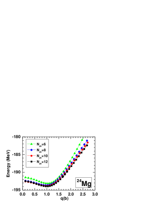
Figure 1: (Color online) Binding energy curves for ²⁴Mg, calculated by the constrained self-consistent triaxial relativistic mean-field approach in a three-dimensional harmonic oscillator basis with major shells $N_{\rm sh}=6,8,10$, and 12 respectively.

In Fig. 1, we show the mean-field binding energy curves for ²⁴Mg as functions of the mass quadrupole moment $q$ ($q_{22}=0$) defined in Eq. (27), calculated by the triaxial RMF-PC approach with the parameter set PC-F1. The four different energy curves correspond to the calculations with $N_{\rm sh}=6,8,10$, and $12$ major oscillator shells respectively. It shows that $N_{\rm sh}=8$ is sufficient to obtain a reasonably converged mean-field binding energy curve for ²⁴Mg. Pairing correlations have been taken into account by the BCS method with monopole pairing forces. The pairing strength parameters $G_{\tau}$ are determined separately for neutrons and protons by adjusting the pairing gaps of the mean-field ground state to the odd-even mass difference as obtained with a five-point formula. The pairing strength parameters $G_{n}=34.6/A$ MeV and $G_{p}=33.75/A$ MeV determined in this way have been kept fixed throughout the constraint calculations.

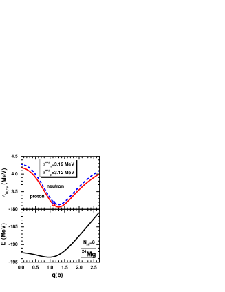
Figure 2: (Color online) Upper panel: Pairing gaps $\Delta_{\tau=n/p}$ of neutron (dash line) and proton (solid line). Lower panel: energy curve for ²⁴Mg in a triaxial RMF-PC+BCS calculation with a constant pairing strength $G_{\tau}$, determined by fitting the ground state gaps $\Delta_{\tau}$ to the odd-even mass difference.

In Fig. 2 we plot the pairing gaps of neutrons and protons in ²⁴Mg as functions of the quadrupole moment $q$ ($q_{22}=0$) together with the corresponding energy curve. The total energy shows a prolate deformed minimum in the energy curve at $q=1.04$ with $E_{\mathrm{tot.}}=-193.57$ MeV. This figure indicates clearly that the pairing gap changes considerably with the deformation reflecting the changes in the single particle level density. Obviously the minimum in the energy corresponds to a rather low level density Ring80 .

For an axially symmetric intrinsic state, the norm overlap in Eq. (88) can be calculated analytically using the Gaussian Overlap Approximation (GOA) Onishi66 ; Beck70 :

$$n(q,q;0,\theta,0)\approx\exp[-\frac{1}{2}\langle\hat{J}^{2}_{y}\rangle\sin^{2}\theta],$$ (65)

which turns out to be an excellent approximation and thus provides a very useful test of the numerical procedure used in angular momentum projection Niksic06I .

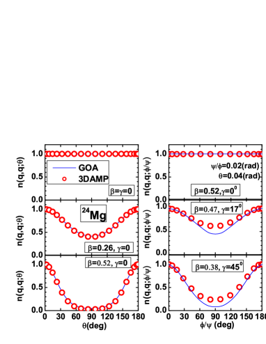
Figure 3: (Color online) Left panel: A comparison between the norm overlaps $n(q,q;\theta)$ as functions of the Euler angle $\theta$ for several intrinsic states of ²⁴Mg obtained by a 3DAMP calculation (open circle) and the GOA formula (solid curve). Right panel: A comparison between the norm overlaps $n(q,q;\phi/\psi)$ as functions of the Euler angles $\phi$ and $\psi$ for several different intrinsic states of ²⁴Mg obtained by a 3DAMP calculation (open circle) and the GOA formula (solid curve), where the Eulers angle are $\psi=0.02$ and $\phi=0.02$ radian with $\theta=0.04$ radian.

Fig. 3 displays the norm overlaps $n(q,q;0,\theta,0)$ as functions of the Euler angle $\theta$ for several different axially deformed intrinsic states of ²⁴Mg. It shows that the 3DAMP calculated values of the function $n(q;\theta)$ are in good agreement with those given by the GOA approximation.

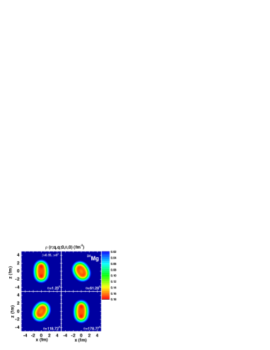
Figure 4: (Color online) The mixed densities $\rho(\bm{r};q,q;\phi,\theta,\psi)$ in $x$-$z$ plane with $\beta=0.55,\gamma=0^{\circ}$. The Euler angle $\theta$ has the value of $1.23^{\circ}$, $61.28^{\circ}$, $118.72^{\circ}$, and $178.77^{\circ}$ respectively keeping $\phi=\psi=0$.

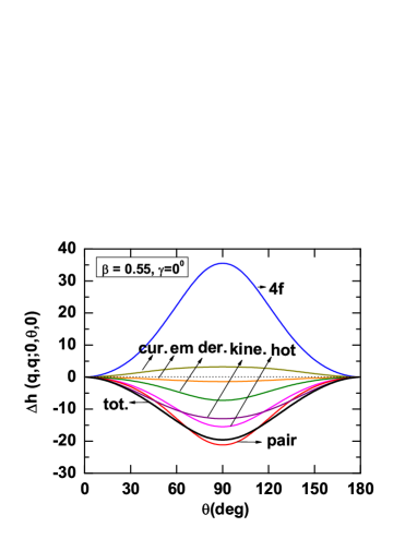
Figure 5: (Color online) The different terms of the Hamiltonian overlap for $\beta=0.55$ and $\gamma=0^{\circ}$ as functions of the Euler angle $\theta$ normalized to $\theta=0^{\circ}$.

For triaxially well-deformed intrinsic states, the norm overlap has been derived approximately in Refs. Beck70 ; Islam79 :

$$n(q,q;\phi,\theta,\psi) \approx \exp[-\frac{1}{2}\langle\hat{J}^{2}_{y}\rangle\theta^{2}+(\cos(\phi+\psi)-1)\langle\hat{J}^{2}_{z}\rangle$$ (66)

$$+\frac{i}{2}\langle\hat{J}_{x}\rangle\theta(\sin\phi-\sin\psi)].$$

In our calculation for ²⁴Mg, the third term in the exponential vanishes because of time reversal invariance $\langle\hat{J}_{x}\rangle=0$. The norm overlaps $n(q,q;\phi/\psi)$ are given in Fig. 3 as functions of the Euler angles $\phi$ and $\psi$ for several triaxially deformed intrinsic states of ²⁴Mg. It is found that the norm overlaps $n(q,q;\phi/\psi)$ oscillate in an exact 3DAMP calculation as functions of $\phi$ and $\psi$ with a period of $T=180^{\circ}$. The approximate formula Eq. (66) is obviously valid only in the interval $0^{\circ}$ to $90^{\circ}$. In order to obtain the approximate results in the interval between $90^{\circ}$ and $180^{\circ}$ we use symmetry around the angle $\phi/\psi=90^{\circ}$. In this case, Fig. 3 shows that the Gaussian overlap approximation can roughly reproduce the results obtained by the exact 3DAMP calculations. Moreover, as expected, the larger the $\gamma$ deformation of the intrinsic state is, the larger is the amplitude of the oscillating norm overlaps $n(q;\phi/\psi)$.

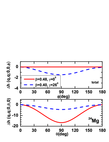
Figure 6: (Color online) Upper panel: Hamiltonian overlap with $\beta=0.48,\gamma=0^{\circ}$ as a function of the Euler angle $\theta$. Lower panel: Hamiltonian overlap with $\beta=0.40,\gamma=26^{\circ}$ as a function of the Euler angles $\phi$ and $\psi$. The values with $\theta=0$ or $\phi$( or $\psi)=0$ are chosen as zero.

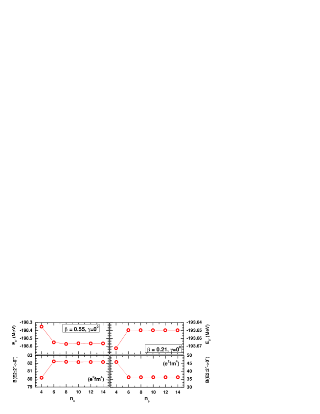
Figure 7: (Color online) The projected energy of the lowest $0^{+}$ state derived from mean-field states with $\beta=0.55,\gamma=0$ and $\beta=0.21,\gamma=0^{\circ}$ for the nucleus ²⁴Mg, and the $B(E2\downarrow:2^{+}\rightarrow 0^{+})$ transition probability, as functions of the number of mesh points $n_{\theta}$ for the Euler angle $\theta$.

To describe the collective motion of nuclei in the context of energy density functional theory, one should determine the corresponding collective Hamiltonian. In the 3DAMP+RMF-PC approach, the matrix elements of collective Hamiltonian are constructed in Eq. (II.2) in terms of the Hamiltonian overlaps, which have their standard functional form but depend upon the mixed densities and currents.

In Fig. 4, we plot the mixed nucleon densities $\rho({\bm{r}};q,q;\phi,\theta,\psi)$ in the $x$-$z$ plane derived from the mean-field state with $\beta=0.55,\gamma=0^{\circ}$ for $\phi=\psi=0^{\circ}$ and for various Euler angles $\theta=$ $1.23^{\circ}$, $61.28^{\circ}$, $118.72^{\circ}$, and $178.77^{\circ}$. It is obvious that the reflection symmetries with respect to the planes $x=0$, $y=0$ and $z=0$ present in the mean-field densities are violated in the corresponding mixed densities. Moreover, we show in Fig. 5 the various terms in the Hamiltonian overlap $h(q_{a},q_{a};\Omega)\equiv{}_{a}\langle 0|\hat{H}|\Omega\rangle_{a}$ resulting from the four-fermion coupling term, the current contributions, the Coulomb term, the derivative term, the kinetic term, the higher order term and the pairing term as functions of the Euler angle $\theta$ for the mean-field state at the point $\beta=0.55,\gamma=0^{\circ}$. The energy surface is normalized to $\theta=0$, i.e. $\Delta h(q_{a},q_{a};\Omega)=h(q_{a},q_{a};\Omega)-h(q_{a},q_{a};0)$. We find that the current contributions and the Coulomb term in the Hamiltonian overlap change mildly with the rotation angle $\theta$ and thus they have only small contributions to the collective Hamiltonian. On the contrary, the four-fermion coupling term, the pairing term and the higher order term are sensitive to the Euler angle $\theta$ and play a dominant role in the collective Hamiltonian.

In Fig. 6, we display the total Hamiltonian overlap for the axially deformed mean-field state with $\beta=0.48,\gamma=0^{\circ}$ and the triaxially deformed mean-field state with $\beta=0.40,\gamma=26^{\circ}$ as functions of the Euler angle $\theta$, or the Euler angles $\phi$ and $\psi$. It shows that both for the axially deformed shape and the triaxially deformed shape, the Hamiltonian overlaps, behaving like the norm overlaps, oscillate with the period $T=180^{\circ}$ in the Euler angle $\theta$, $\phi$, or $\psi$.

A N-point Gaussian-Legendre quadrature is used for integration over the Euler angles $\phi,\theta$ and $\psi$ in the calculations of the norm kernel $\mathcal{N}^{J}_{KK^{\prime}}$ and the Hamiltonian kernel $\mathcal{H}^{J}_{KK^{\prime}}$. The calculation of the Hamiltonian overlap at each mesh point of the Euler angles is very time consuming. Therefore, besides the utilization of symmetries in overlaps, it is essential to make a careful check of the convergence for the number of mesh points. The projected energy and the $B(E2)$ transition probability are good observables for this purpose.

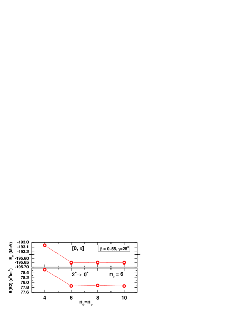
Figure 8: (Color online) The projected energy of the first $0^{+}$ state obtained from the mean-field state with $\beta=0.55,\gamma=28^{\circ}$ for ²⁴Mg, and the $B(E2\downarrow:2^{+}\rightarrow 0^{+})$ transition probability, as functions of the number of mesh points $n_{\phi}$ (or $n_{\psi}$) for the Euler angles $\phi$ (or $\psi$).

In Fig. 7, we plot the projected energy of first $0^{+}$ state obtained from the mean-field states with $\beta=0.55,\gamma=0^{\circ}$ and $\beta=0.21,\gamma=0^{\circ}$ for ²⁴Mg, and the corresponding $B(E2\downarrow:2^{+}\rightarrow 0^{+})$ transition probabilities as functions of the number of mesh points $n_{\theta}$ for the Euler angle $\theta$. The projected energy of the $0^{+}$ state from the mean-field states with $\beta=0.55,\gamma=28^{\circ}$ and the $B(E2\downarrow:2^{+}\rightarrow 0^{+})$ transition probability, as functions of the number of mesh points $n_{\phi}$ (or $n_{\psi}$) for the Euler angle $\phi$ (or $\psi$) are shown in Fig. 8, where $\theta$, $\phi$ and $\psi$ have values between 0 and $\pi$. We find that in order to achieve a precision of $0.001\%$ for $E_{0^{+}}$ and $0.1\%$ for $B(E2:2^{+}\rightarrow 0^{+})$ the total number of mesh points for the Euler angles in the intervals $\phi\in[0,\pi]$, $\theta\in[0,\pi]$, $\psi\in[0,\pi]$ should fulfil the relation: $N_{\phi}\times N_{\theta}\times N_{\psi}\geq 6\times 6\times 6$.

Figure 9: (Color online) The projected energies of $2^{+},4^{+}$ and $6^{+}$ states from the mean-field states with $\beta=0.47,\gamma=17^{\circ}$ and $\beta=0.52,\gamma=0^{\circ}$ for ²⁴Mg as functions of the number of mesh points $n_{\phi}$ (or $n_{\psi}$) or $n_{\theta}$. $E^{J}_{0}$ is the converged energy of a state with spin $J$.

Figure 10: (Color online) The projected energy of $0^{+}$ state from the mean-field solution with $\beta=0.55,\gamma=0^{\circ}$ for ²⁴Mg, and the $B(E2\downarrow:2^{+}\rightarrow 0^{+})$ transition probability, as functions of cut-off $\zeta$ in Dirac space ).

According to the uncertainty principle $\Delta J\cdot\Delta\Omega\simeq\hbar$, we need a large number for meshpoints in the Euler angels for higher values of the spin. In Fig. 9, we show the projected energies of $2^{+},4^{+}$ and $6^{+}$ obtained from the mean-field states with $\beta=0.47,\gamma=17^{\circ}$ and $\beta=0.52,\gamma=0^{\circ}$ as functions of the number of mesh points $n_{\phi}$, $n_{\psi}$ and $n_{\theta}$. We find that it is possible with $N_{\phi}\times N_{\theta}\times N_{\psi}\geq 12\times 14\times 12$, to achieve a precision of $0.001\%$ in the energy of a projected state with angular momentum up to $J=6$ in the ground state band. In the following calculations we use such large numbers of mesh points in the Euler angles.

Since the states with very small occupation probabilities give negligible contributions to the kernels, as usual, we introduce a cut-off parameter $\zeta$, which divides the Dirac space into an occupied part and an unoccupied part (see Eq. (80). The states with $v^{2}_{k}\leq\zeta$ will be excluded in the calculation of the overlaps. In Fig. 10 we show the projected energy of the first $0^{+}$ state and the $B(E2\downarrow:2^{+}\rightarrow 0^{+})$ transition probability projected from the mean-field state with $\beta=0.55,\gamma=0^{\circ}$ as functions of the cut-off parameter $\zeta$. It shows that $\zeta$ should be chosen as $\zeta\leq 10^{-8}$ in order to get a precision of $0.01\%$ for $E_{0^{+}}$ and of $0.00001\%$ for the $B(E2\downarrow:2^{+}\rightarrow 0^{+})$ value. Using the cut-off $\zeta$ reduces the computational effort ( about 80% of total computer time for $N_{\rm sh}=8$) in the calculations of the norm overlap and the matrix elements of mixed densities and pairing tensors considerably, especially for the cases of large $N_{\rm sh}$, small particle number and weak pairing, where most single particle levels of the Dirac basis have nearly zero occupation probabilities.

III.3 Tests of three-dimensional angular momentum projection

III.3.1 Application to an axially deformed shape

To illustrate the validity of our newly-developed 3DAMP+RMF-PC+BCS code, we first apply it to the axially deformed case, where a 1DAMP calculation is possible. The projected $J^{\pi}$ = $0^{+}$, $2^{+}$, $4^{+}$, $6^{+}$, and $8^{+}$ potential energy curves of ³²Mg have already been calculated with 1DAMP+RMF-PC+BCS approach in Ref. Niksic06I . To make a comparison, we perform the same calculations within the 3DAMP+RMF-PC+BCS approach. The numerical techniques are the same as those of Ref. Niksic06I . We find that our newly-developed 3DAMP+RMF-PC+BCS code can reproduce the results given by 1DAMP+RMF-PC+BCS approach.

Furthermore, following Ref. Bender08 , we first test the 3DAMP+RMF-PC approach for an axially deformed shape, which allows two distinct orientations in the intrinsic frame: the symmetry axis can either parallel to the $z$-axis or it can be perpendicular to it.

Figure 11: (Color online) The excitation spectra and $B(E2)$ values projected from the axially deformed mean-field states with $\beta=0.44,\gamma=180^{0}$ and $\beta=0.44,\gamma=60^{0}$ respectively. The first and second columns show the unique band with $K=0$ and the unique band with $K$-mixing. The last four columns show the decomposition into $K$-components when the symmetry axis is chosen perpendicular to the $z$ axis, i.e. the $K=0,2,4,6$ bands respectively.

Figure 12: (Color online) Upper panel: The probabilities $W^{J}$ of finding the component with given spin $J$. Lower panel: the probabilities $W^{J}_{K}$ of finding the component with given spin $J$ and the projection $K$ along the $z$-axis in the mean-field state with the deformation parameters $\beta=0.44,\gamma=60^{\circ}$.

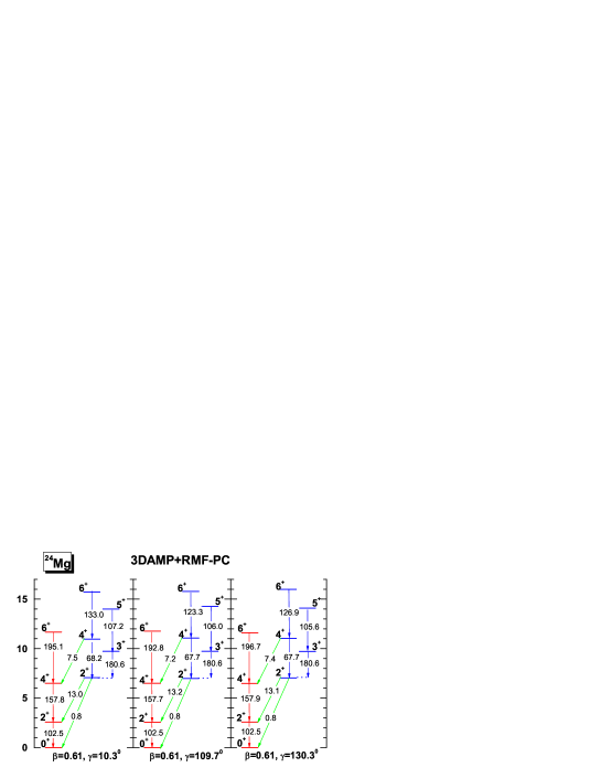
Figure 13: (Color online) The excitation spectra and $B(E2)$ values projected from triaxially deformed mean-field states with $\beta=0.61,\gamma=10.3^{0}$; $\beta=0.61,\gamma=109.7^{0}$; and $\beta=0.61,\gamma=130.3^{0}$ respectively.

In Fig. 11, we show the excitation spectra and $B(E2)$ values for ²⁴Mg projected from the axially deformed mean-field states with $\beta=0.44,\gamma=180^{0}$ and $\beta=0.44,\gamma=60^{0}$ respectively. For $\gamma=180^{0}$, $z$-axis is along the symmetry axis, and therefore only one pure $K=0$ band can be found. All other $K$-components have zero norm. While for $\gamma=60^{0}$, one can show that the pure $K=0$ state is transformed into a multiplet of states with $K$ ranging between 0 and $J$. Such phenomena can be seen more clearly from the probabilities $W^{J}\equiv\sum_{K}\langle\Phi(q)|\hat{P}^{J}_{KK}|\Phi(q)\rangle$ of finding a component with given spin $J$ and the probabilities $W^{J}_{K}\equiv\langle\Phi(q)|\hat{P}^{J}_{KK}|\Phi(q)\rangle/W^{J}$ of finding a component with given spin $J$ as well as given projection $K$ along $z$-axis. These probabilities are shown in Fig. 12.

In principle, the transformed wave functions differ only by an unobservable phase and the energies of projected states as well as the electromagnetic transition probabilities should be identical. This provides us an excellent test of the numerical accuracy of the projection scheme in the code. Fig. 11 shows that for the low spin states, e.g., $0^{+},2^{+}$, the projected energies and $B(E2)$ values are exactly the same. As angular momentum increases, the difference increases to a largest value ($\sim 0.4\%$) in the $B(E2\downarrow:6^{+}\to 4^{+})$, which could be reduced with more mesh points in the Euler angles.

III.3.2 Application to a triaxially deformed shapes

The excitation energies and $B(E2)$ values for ²⁴Mg projected from the triaxially deformed mean-field states with $\beta=0.61,\gamma=10.3^{0}$; $\beta=0.61,\gamma=109.7^{0}$ and $\beta=0.61,\gamma=130.3^{0}$ are presented in Fig. 13. All the excitation energies are arranged into bands according to the $B(E2)$ values. These three intrinsic states correspond to the same nuclear shape with three different orientations in the intrinsic frame. The projected energy and the electromagnetic transition probability do not depend on the orientation of the nucleus and therefore, in principle, the predicted values should be the same as illustrated in Fig. 13. It shows that the projected energies and $B(E2)$ values in these cases are in good agreement with each other. However, small differences in the $B(E2)$ values appear and increase with angular momentum. Except for the $B(E2:6^{+}\rightarrow 4^{+})$ in the $K=2$ band, the difference is smaller than $1\%$. This indicates that more mesh points in the Euler angles are necessary to provide a better description of the $B(E2:6^{+}\rightarrow 4^{+})$.

Figure 14: (Color online) The probabilities $W^{J}$ in the mean-field states with $\beta=0.61,\gamma=10.3^{0}$, $\beta=0.61,\gamma=109.7^{0}$, and $\beta=0.61,\gamma=130.3^{0}$ respectively.

The decomposition of a triaxial mean-field state into components with different $J$-values in the laboratory frame should also be independent on its orientation in the intrinsic frame. In Fig. 14, we show almost the same probabilities $W^{J}$ of different spin states in these cases.

III.3.3 Dispersion of particle numbers

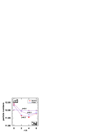
Figure 15: (Color online) The average neutron (filled circle) and proton (open circle) numbers of angular momentum projected states with $J\leq 6$ from axially deformed intrinsic states of ²⁴Mg with $\beta=0.2,0.3,0.4$.

Although the mean-field intrinsic states are obtained with the constraint on the right average particle number, it cannot guarantee the right particle number in the angular momentum projected states. In order to make up this flaw, in principle, one has to perform PNP calculation. The study with both PNP and 3DAMP in the context of GCM has only been attempted based on a Skyrme EDF theory Bender08 . Such kind of study based on a covariant EDF theory is still extremely time-consuming. As the first step, in this work, neither the exact projection on particle numbers $N$ and $Z$, nor a constrain on the average number of particle in the angular-momentum projected states is performed. Therefore, it is essential to know the dispersion of particle numbers within a rotational band. In Fig. 15, we plot the average neutron and proton numbers of angular momentum projected states with $J\leq 6$ from axially deformed intrinsic states of ²⁴Mg with $\beta=0.2,0.3,0.4$. It shows that the error in average particle number of projected states with $J\leq 6$ is within $0.5\%$.

III.4 Examples of three-dimensional angular momentum projection

III.4.1 Application to ²⁴Mg

Table 2: Reduced $E2$ transition probabilities from states $J^{\pi}_{i}$ to states $J^{\pi}_{f}$ in ²⁴Mg. The minimum of the projected $J=2$ PES is used for the calculation of intrinsic wave function. The experimental data for the excitation energies $E_{\rm x}$ [in units of MeV] and $E2$ transition probabilities [in units of e²fm⁴] are taken from most recent available sources. 1e²fm${}^{4}=4\pi(\frac{5}{3})^{2}(1.2A^{1/3})^{-4}$ W.u. $=0.243$ W.u. for ²⁴Mg.

$J^{\pi}_{i}$	$E_{xi}$(Exp.)	$J^{\pi}_{f}$	$E_{xf}$(Exp.)	$B(E2)_{\rm Exp.}$	$B(E2)_{\rm The.}$
$2^{+}_{1}$	1.37	$0^{+}_{1}$	0.0	$86.4\pm 1.6$	74.5
$4^{+}_{1}$	4.12	$2^{+}_{1}$	1.37	$155.6\pm 12.3$	104.9
$6^{+}_{1}$	8.11	$4^{+}_{1}$	4.12	$156.4\pm 53.5$	131.3
$2^{+}_{2}$	4.24	$0^{+}_{1}$	0.0	$6.6\pm 0.4$	12.3
$2^{+}_{2}$	4.24	$2^{+}_{1}$	1.37	$12.3\pm 2.1$	32.1
$3^{+}_{2}$	5.24	$2^{+}_{1}$	1.37	$9.5\pm 0.8$	21.4
$3^{+}_{2}$	5.24	$4^{+}_{1}$	4.12	$<17.7$	32.5
$4^{+}_{2}$	6.01	$2^{+}_{1}$	1.37	$4.1\pm 0.8$	21.8
$4^{+}_{2}$	6.01	$4^{+}_{1}$	4.12	$4.1\pm 4.1$	21.0
$6^{+}_{2}$	9.53	$4^{+}_{1}$	4.12	$2.5\pm 1.2$	0.4
$3^{+}_{2}$	5.24	$2^{+}_{2}$	4.24	$156.4\pm 22.6$	134.2
$4^{+}_{2}$	6.01	$2^{+}_{2}$	4.24	$77.0\pm 9.9$	63.0
$5^{+}_{2}$	7.81	$3^{+}_{2}$	5.24	$144.0\pm 20.3$	103.7
$6^{+}_{2}$	9.53	$4^{+}_{2}$	6.01	$74.2\pm 32.9$	44.9

The 3DAMP+RMF-PC approach has been used in Ref. Yao08cpl2 to describe the PES in the $\beta$-$\gamma$ plane for the lowest $J^{\pi}=0^{+}$ state and for the first excited $J^{\pi}=2^{+}$ in the nucleus ²⁴Mg. There is no pronounced minimum with an obvious $\gamma$-deformation in the PES for the $0^{+}$ state, which is in disagreement with the results of Ref. Bender08 , where a 3DAMP+PNP calculation based on a non-relativistic Skyrme HFB functional shows a pronounced triaxial minimum with $\beta=0.6$ and $\gamma=16^{\circ}$. Keeping in mind that we found strong pairing gaps in our mean-field calculations, an additional number projection is not expected to change this result. A possible reason for this difference is the fact that different energy functionals are used in these two calculations. A minimum with $\beta\approx 0.55,~{}\gamma\approx 10^{\circ}$ has been found on the PES of the first excited $2^{+}$ state. To construct the excitation spectrum and to calculate $B(E2)$ transitions, one should in principle perform a GCM configuration mixing calculation on top of three-dimensional angular momentum projection, or choose the minimum of the different $J$ projected PES as basis. However, such kind of calculations are beyond our present study. Instead, we use the minimum of the projected $J=2$ PES as basis to calculate the experimentally observed excited energy levels and the $B(E2)$ transition probabilities in ²⁴Mg using Eqs. (39) and (LABEL:E42). This is the only way to obtain $K=2$ bands in our calculation. The details about the $B(E2)$ transition probabilities in ²⁴Mg are given in Tab. 2. It shows that the predicted intraband $B(E2)$ values are systematically smaller than the data, while the interband $B(E2)$ values are systematically overestimated. It indicates that the amplitude of “K-mixing” is too strong in our calculations.

Figure 16: (Color online) The probabilities $W^{J}$ and the probabilities $W^{J}_{K}$ in mean-field states with $\beta=0.55$ as functions of triaxial deformation $\gamma$.

In order to understand the effect of $\gamma$-deformation on the amplitude of angular momentum mixing, it is useful to investigate the individual components forming the intrinsic state $|\Phi(q)\rangle$, i.e. the $J$- and $K$-mixing. In Fig. 16, we present the probabilities $W^{J}$ and the probabilities $W^{J}_{K}$ in the mean-field states with $\beta=0.55$ as functions of the triaxiality parameter $\gamma$, ranging between $0^{\circ}$ and $60^{\circ}$. It is noted that each $\gamma$-deformation in this range corresponds to a definite shape uniquely. Fig. 16 shows that the $J$-mixing remains practically constant with changes in the $\gamma$-deformation, while the amount of $K$-mixing increases considerably with increasing triaxiality. This indicates that the underestimated intraband $B(E2)$ values and the overestimated interband $B(E2)$ in the low-lying excited states of ²⁴Mg as shown in Tab. 2 are due to the large $\gamma$-deformation in the intrinsic state.

To illustrate the effect of $\gamma$-deformation on the $B(E2\downarrow$) values, we plot in Fig. 17 the intraband $B(E2\downarrow$) transition probabilities for $2^{+}_{1}\to 0^{+}_{1}$, $4^{+}_{1}\to 2^{+}_{1}$ and $6^{+}_{1}\to 4^{+}_{1}$ in the ground state band projected from mean-field states with $\beta=0.55$ as functions of the $\gamma$-deformation. Obviously the intraband $B(E2\downarrow$) values increase when $\gamma$ approaches $0^{\circ}$ or $60^{\circ}$. It indicates that a configuration mixing calculation (GCM) within a generator coordinate method might be very important to understand the observed $B(E2$) values. Alternatively, calculating $B(E2)$ value using the minima of each $J$ projected PES might also improve the results. Moreover, we note here that in contrast to the $B(E2\downarrow$) values for the $4^{+}_{1}\to 2^{+}_{1}$ and $6^{+}_{1}\to 4^{+}_{1}$ transitions with obvious minima at $\gamma=10^{\circ}$, $B(E2\downarrow$) values for $2^{+}_{1}\to 0^{+}_{1}$ changes only moderately with $\gamma$, ranging from $72$ e²fm⁴ to $88$ e²fm⁴, which is consistent with the data $86.4\pm 1.6$ e²fm⁴ of Ref. Keinonen89 .

Figure 17: (Color online) $B(E2\downarrow$) transition probabilities for $2^{+}_{1}\to 0^{+}_{1}$, $4^{+}_{1}\to 2^{+}_{1}$ and $6^{+}_{1}\to 4^{+}_{1}$ in the ground state band, projected from the mean-field state with $\beta=0.55$ in the nucleus ²⁴Mg, as functions of the triaxial deformation $\gamma$.

III.4.2 Application to ³⁰Mg

The evolution of shell structure and appearance of new magic numbers in neutron-rich nuclei has become one of the main topics in recent investigations of nuclear structure physics. Especially, the erosion of the neutron magic numbers $N=20$ and 28 and the occurrence of well-deformed prolate deformed structures in such magic or close-to-magic nuclei are presently in the focus of several investigations.

There is much controversy about the deformation of the ground state in the nucleus ³⁰Mg. Experimentally, this deformation is determined by measuring the $B(E2;0^{+}_{\rm gs}\rightarrow 2^{+})$ transition probability. The values obtained at MSU and at GANIL using the method of intermediate-energy Coulomb excitation are 295(26) e² fm⁴ Pritychenko99 and 435(58) e² fm⁴ Chiste01 , respectively. However, the most recent measurement performed at CERN results in 241(31) e² fm⁴ Niedermaier05 , which is lower than those extracted in previous measurements performed at intermediate energies. Therefore it is very interesting to study this problem theoretically within the present approach.

In Fig. 18 we plot the potential energy surfaces of mean-field states and projected $0^{+}$ states in the $\beta$-$\gamma$ plane for the nucleus ³⁰Mg. The intrinsic states are calculated in the triaxial RMF-PC+BCS approach using monopole pairing forces with $G_{n}=24.4/A$, $G_{p}=29.7/A$, adjusted to the experimental odd-even mass differences. We find that the mean-field potential energy surface is very soft against $\beta$ in the spherical region. It is hard to recognize a minimum. The energy surface projected on the $0^{+}$-state has, however, a pronounced axially symmetric minimum.

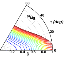
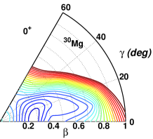
Figure 18: (Color online) The potential energy surfaces of mean-field state and projected $0^{+}$ states in the $\beta$-$\gamma$ plane obtained by triaxial RMF-PC+BCS calculations for the nucleus ³⁰Mg. The contour lines are separated by $0.5$ MeV.

Fig. 19 shows axially symmetric results for the nucleus states in ³⁰Mg. The corresponding potential energy curves of the intrinsic states and of the projected $J^{\pi}=0^{+},2^{+},4^{+},6^{+}$ states are given as functions of the quadrupole moment $q$ ($q_{22}=0$). The intrinsic deformed states are obtained in the RMF-PC+BCS approach using either a monopole pairing forces or a zero range $\delta$-type pairing forces. We find that the projected curves for the $0^{+}$ state have in both cases an obvious minimum at $\beta\simeq 0.25$. The energy differences between the minimum and the spherical shape are 3.87 MeV (BCS-G) and 3.69 MeV (BCS-$\delta$) respectively. The corresponding $B(E2:0^{+}\rightarrow 2^{+})$ values are $194.8$ e²fm⁴ and $194.6$ e²fm⁴, respectively. Both of them are somewhat smaller than the data.

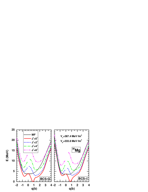
Figure 19: (Color online) Potential energy curves of the projected $J^{\pi}=0^{+},2^{+},4^{+},6^{+}$ states in ³⁰Mg, as functions of the quadrupole moment $q$. The intrinsic deformed states are obtained by RMF-PC+BCS calculations with both monopole pairing forces (left panel) and $\delta$-type pairing forces (right panel). The pairing strength parameters $V_{\tau}$ for the zero range pairing forces are adjusted the experimental pairing gap as discussed in Eq. (23).

III.4.3 Application to ³²Mg

For the nucleus ³²Mg, a much lower excitation energy of 0.885 MeV was measured for the first $2^{+}$-state Mueller84 and a large deformation with $\beta\simeq 0.51$ has been inferred from the measured B(E2: $0^{+}\rightarrow 2^{+}$) value ($454\pm 78$ e²fm⁴) Motobayashi95 . Therefore this nucleus has drawn much attention in studies with self-consistent approaches. Corrections from the angular momentum projection and configuration mixing are found to be essential to reproduce the large deformed ground state of ³²Mg in the HFB approach with the Gogny force D1S Guzman00plb ; Guzman00prc . However, similar non-relativistic calculation with Skyrme-type the Sly4 force Heenen00 and relativistic calculation with the PC-F1 force fail to reproduce the data Niksic06I . Therefore, it is interesting to revisit this problem within our 3DAMP+RMF-PC approach.

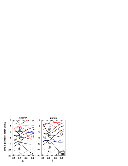
Figure 20: (Color online) The neutron (left panel) and proton (right panel) single-particle levels for ³²Mg, as functions of the quadrupole deformation $\beta$. The levels with positive (negative) parity are shown with solid (dashed) lines. The levels belonging to the $f_{7/2}$ orbit are plotted with red dashed lines. The fermi energies for neutrons and protons are plotted with blue dotted lines.

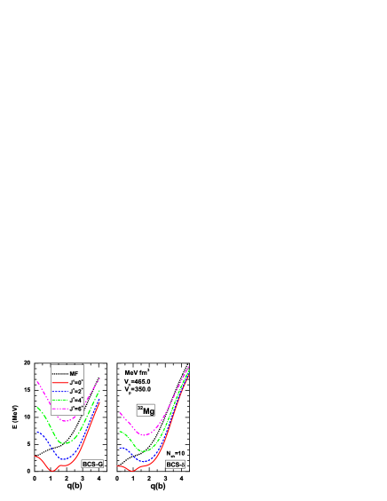
Figure 21: (Color online) Potential energy curves of the projected $J^{\pi}=0^{+},2^{+},4^{+},6^{+}$ states in ³²Mg, as functions of the quadrupole moment $q$. The intrinsic deformed states are obtained by RMF-PC+BCS calculations with monopole forces (left panel) and $\delta$-forces (right panel). The pairing strength parameters $V_{\tau}$ for the zero range pairing forces are adjusted the experimental pairing gap as discussed in Eq. (23).

Fig. 20 displays the neutron and proton RMF-PC+BCS single-particle energy levels for ³²Mg as functions of the quadrupole deformation $\beta$. The pairing strength parameters are $G_{n}=26.78/A$ and $G_{p}=32.25/A$ for the monopole pairing force. They are obtained by adjusting the gaps at the spherical minimum (the ground state of the mean-field calculation) to the experimental odd-even mass difference with a five-point formula. In the self-consistent calculations we find a collapse of proton pairing for the range $0.45<\beta<0.75$.

The potential energy curves of the projected $J^{\pi}=0^{+},2^{+},4^{+},6^{+}$ states in ³²Mg are plotted in Fig. 21 as functions of the quadrupole moment $q$ ($q_{22}=0$). The intrinsic deformed states are obtained from RMF-PC+BCS calculations with monopole forces and $\delta$-forces. The pairing strengthes $V_{\tau}$ are adjusted to the odd-even mass difference.

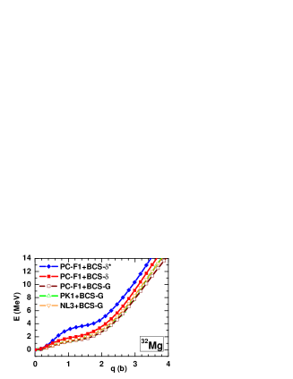
Figure 22: (Color online) The energy curves as functions of mass quadruple moment $q$ ($\gamma=0^{\circ}$) for ³²Mg, calculated with different RMF parameterizations.

At the mean-field level, a shoulder of only 1.8 MeV above the spherical minimum has been found in the present calculations with pairing strength parameters adjusted to odd-even mass differences. This value is close to the prediction of 1.9 MeV for the shoulder by the HFB approach with the Gogny force Guzman02npa , but much smaller than the value of 3.5 MeV predicted by the RMF-PC model with $\delta$ pairing forces taken from the parameter set PC-F1 set Niksic06I . In Fig. 22 we show various RMF calculations for this shoulder with the parameter sets PC-F1 Niksic06I , PK1 Long04 and NL3 Lalazissis97 . Pairing correlations are taken into account by the BCS method with a monopole pairing force (BCS-G) or a $\delta$-force (BCS-$\delta$). In all cases the pairing strength parameters are adjusted to the odd-even mass difference except the case labeled by “BCS-$\delta$*” where $V_{\tau}$ has bee taken from the PC-F1 set Niksic06I .

We find that the energy curves in RMF calculations do not depend on too much on the effective interactions but rather strongly on the strength of the pairing force. All the calculations with a pairing strength adjusted to the experimental pairing gaps give a lower shoulder, while the calculation with a $\delta$-pairing forces taken from the PC-F1 set produce a higher shoulder with a stiffer energy surface against quadrupole deformation $\beta$. Similar phenomena have also been found in Skyrme-Hartree-Fock+BCS calculations Guzman07 . As a consequence, one will obtain different predictions for the deformation of ground state for different pairing correlations. More detailed investigations concerning this question are in progress.

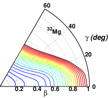
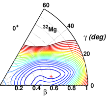
Figure 23: (Color online) The potential energy surfaces of mean-field theory (left panel) and of angular momentum projection $J=0$ after the variation (right panel) in the $\beta$-$\gamma$ plane obtained by triaxial RMF-PC+BCS calculations for ³²Mg. The quadrupole deformation of the minimum in potential energy surface of $0^{+}$ state is $\beta\simeq 0.6,\gamma\simeq 10^{\circ}$. The contour lines are separated by $0.5$ MeV.

In Fig. 23 we examine the potential energy surface in the $\beta$-$\gamma$ plane for ³²Mg. Triaxial RMF-PC+BCS calculations with a monopole pairing force (left panel) are compared with angular momentum projection on $J=0$. We observe that considering the $\gamma$-degree of freedom one can expect considerably enlarged ground state deformations. The quadrupole deformation of the minimum in the angular projected $0^{+}$ PES is found to be at $\beta\simeq 0.6,\gamma\simeq 10^{\circ}$, based on which, the predicted energy of the $2^{+}$ state is $E=1.21$ MeV and the predicted B(E2: $0^{+}\rightarrow 2^{+}$) value is $573.5$ e²fm⁴. It has to be pointed out that the PES of $0^{+}$ state is very $\beta$-soft in the region $0.3\leq\beta<0.7$. Based on the intrinsic state with quadrupole deformations $\beta=0.3,\gamma=0$, the AMP predicted an energy of $2^{+}$ is $E=3.39$ MeV and a B(E2: $0^{+}\rightarrow 2^{+}$) value of $250.2$ e²fm⁴. This indicates clearly that the generator coordinate method based on 3DAMP approach becomes necessary for a full understanding of the properties of ³²Mg.

IV Summary and perspective

In this paper, a full three-dimensional angular momentum projection on top of a triaxial relativistic mean-field calculation has been implemented for the first time. The underlying Lagrangian is a point coupling model and pairing correlations are taken into account both with a monopole force and a $\delta$-force. Convergence has been checked and the validity of this newly-developed approach has been illustrated by applying it to the description of the low-lying excited states in several Mg isotopes.

For ²⁴Mg no pronounced minimum with obvious triaxial deformation has been found on the potential energy surface of the $0^{+}$ state. A minimum with $\beta\approx 0.55,~{}\gamma\approx 10^{\circ}$ has been found on the PES of the first $2^{+}$ state. Using this minimum as a basis for the projection the experimentally observed excitation energies and B(E2) transition probabilities can be qualitatively reproduced. However, the predicted spacing between the levels is overestimated in this approach.

For ³⁰Mg, the projected energy surface of the $0^{+}$ state has a obvious minimum with $\beta\simeq 0.25$. The energy differences between the minimum and the spherical shape are 3.87 MeV (BCS-G) and 3.69 MeV (BCS-$\delta$) respectively. The corresponding $B(E2:0^{+}\rightarrow 2^{+})$ are respectively $194.8$ e²fm⁴ and $194.6$ e²fm⁴.

For ³²Mg, we note that the calculations with adjusted pairing strength parameters produce always a lower shoulder in the mean-field energy curve, which is, together with the triaxial degree of freedom, essential to reproduce the large deformed ground state. Moreover, the mean-field and the projected $0^{+}$ potential energy surfaces of ³²Mg have been found to be very $\gamma$-soft in the region of small deformations and $\beta$-soft in the neighborhood of its minimum.

These investigations indicate that, besides triaxiality, the effects of pairing correlations and shape fluctuations should be treated more carefully in the description of low-lying excited states of exotic nuclei. Work in this direction is in progress.

Finally, we would like to point out that the pairing strength parameters of protons and neutrons in PC-F1 are adjusted to the pairing gaps of the nuclei: ¹³⁶Xe, ¹⁴⁴Sm, ¹¹²Sn, ¹²⁰Sn and ¹²⁴Sn respectively. However, pairing strength parameter obtained in this way might not be well-justified in the region of light nuclei. We have found in the present study for ³⁰Mg: $f_{p}=1.04$, $f_{n}=1.19$ and for ³²Mg: $f_{p}=1.51$, $f_{n}=1.09$, where $f_{\tau}$ is the ratio of the pairing strength parameters of the adjusted delta-pairing and the standard PC-F1 delta-pairing. It indicates that a better parameterizations of the energy density functional is required for the description of light nuclei.

Appendix A Evaluation of contractions and overlaps

The contractions and overlaps have been derived in detail in Ref. Valor00 , where, however, the rotation matrix is assumed to be real from the beginning. This is no longer the case for a three-dimensional angular momentum projection. In addition these earlier investigations were done only for nonrelativistic density functionals. Therefore, we derive here in a similar way the general formulae of the contractions and overlaps suitable for the three-dimensional relativistic case and used in the present numerical applications.

A.1 Determination of the generalized contractions

In the following we derive formulae of generalized contractions $\langle\Phi(q_{a})|\hat{O}\hat{R}(\Omega)|\Phi(q_{b})\rangle$ connecting different intrinsic states. Such formulae can be applied directly in future Generator Coordinate (GCM) calculations with 3DAMP as well.

For convenience, we introduce the following notation

$${}_{a}\langle 0|\equiv\langle\Phi(q_{a})|,\quad|\Omega\rangle_{b}\equiv\frac{\hat{R}(\Omega)|\Phi(q_{b})\rangle}{\langle\Phi(q_{a})|\hat{R}(\Omega)|\Phi(q_{b})\rangle}.$$ (67)

The quasiparticle vacua $|0\rangle_{a}$ and $|\Omega\rangle_{b}$ are defined by the corresponding quasiparticle operators $\alpha_{k}$ and $\beta_{k}$ respectively,

$${}_{a}\langle 0|\alpha^{\dagger}_{k}=0,\quad\beta_{k}|\Omega\rangle_{b}=0.$$ (68)

According to the generalized Wick theorem the contractions $\langle\Phi(q_{a})|\hat{O}\hat{R}(\Omega)|\Phi(q_{b})\rangle$ for an arbitrary many-body operator $\hat{O}$ can be expressed in terms of the mixed densities and mixed pairing tensors

$$\rho_{kl}(q_{a},q_{b};\Omega) \equiv {}_{a}\langle 0|a^{\dagger}_{l}a_{k}|\Omega\rangle_{b},$$ (69a)

$$\kappa^{10}_{kl}(q_{a},q_{b};\Omega) \equiv {}_{a}\langle 0|a_{l}a_{k}|\Omega\rangle_{b},$$ (69b)

$$\kappa^{01}_{kl}(q_{a},q_{b};\Omega) \equiv {}_{a}\langle 0|a^{\dagger}_{k}a^{\dagger}_{l}|\Omega\rangle^{\ast}_{b}.$$ (69c)

In order to derive expressions for these mixed densities we consider the fact that the quasiparticle operators ($\alpha,\alpha^{\dagger}$) and ($\beta,\beta^{\dagger}$) are connected by a Bogoliubov transformation Ring80

$$\begin{pmatrix}\alpha\\ \alpha^{\dagger}\end{pmatrix}=\begin{pmatrix}\mathbb{U}^{\dagger}&\mathbb{V}^{\dagger}\\ \mathbb{V}^{T}&\mathbb{U}^{T}\end{pmatrix}\begin{pmatrix}\beta\\ \beta^{\dagger}\end{pmatrix}.$$ (70)

On the other hand, the quasiparticle operators $\alpha,\alpha^{\dagger}$ are related to the particle operators $a,a^{\dagger}$ by a Bogoliubov transformation,

$$\begin{pmatrix}\alpha\\ \alpha^{\dagger}\end{pmatrix}=\begin{pmatrix}U^{\dagger}_{a}&V^{\dagger}_{a}\\ V^{T}_{a}&U^{T}_{a}\end{pmatrix}\begin{pmatrix}a\\ a^{\dagger}\end{pmatrix}.$$ (71)

In a similar way the quasiparticle operators $\beta,\beta^{\dagger}$ are related to the particle operators $b,b^{\dagger}$ by

$$\begin{pmatrix}\beta\\ \beta^{\dagger}\end{pmatrix}=\begin{pmatrix}U^{\dagger}_{b}&V^{\dagger}_{b}\\ V^{T}_{b}&U^{T}_{b}\end{pmatrix}\begin{pmatrix}b\\ b^{\dagger}\end{pmatrix}.$$ (72)

Assuming that the operators $a,a^{\dagger}$ and $b,b^{\dagger}$ are related by a rotation as Robledo94

$$\begin{pmatrix}a\\ a^{\dagger}\end{pmatrix}=\begin{pmatrix}R(\Omega)&0\\ 0&R^{\ast}(\Omega)\end{pmatrix}\begin{pmatrix}b\\ b^{\dagger}\end{pmatrix},$$ (73)

one finds for the particle operators $a,a^{\dagger}$ and the quasiparticle operators $\beta,\beta^{\dagger}$ the relation

$$\begin{pmatrix}\beta\\ \beta^{\dagger}\end{pmatrix}=\begin{pmatrix}U^{\dagger}_{b}(\Omega)&V^{\dagger}_{b}(\Omega)\\ V^{T}_{b}(\Omega)&U^{T}_{b}(\Omega)\end{pmatrix}\begin{pmatrix}a\\ a^{\dagger}\end{pmatrix},$$ (74)

with the coefficients $U_{b}(\Omega),V_{b}(\Omega)$ given by

$$U_{b}(\Omega)=R(\Omega)U_{b},\quad V_{b}(\Omega)=R^{\ast}(\Omega)V_{b}.$$ (75)

Combining Eq. (71) and Eq. (74) we obtain the matrices $\mathbb{U}$ and $\mathbb{V}$ in Eq. (70)

$$\mathbb{U}^{\dagger} = U^{\dagger}_{a}R(\Omega)U_{b}+V^{\dagger}_{a}R^{\ast}(\Omega)V_{b},$$ (76a)

$$\mathbb{V}^{\dagger} = U^{\dagger}_{a}R(\Omega)V^{\ast}_{b}+V^{\dagger}_{a}R^{\ast}(\Omega)U^{\ast}_{b},$$ (76b)

that relates the quasiparticle operators $\beta,\beta^{\dagger}$ and $\alpha,\alpha^{\dagger}$ and the quasiparticle vacua ${}_{a}\langle 0|$ and $|\Omega\rangle_{b}$ in Eq. (67). With the help of generalized Wick’s theorem Balian69 , one finds the contraction

$${}_{a}\langle 0|\alpha\beta^{\dagger}|\Omega\rangle_{b}=\mathbb{U}^{-1},$$ (77)

and in combination with Eqs. (68), (71) and (74), the elements of the mixed density and the mixed pairing tensors of Eq. (69) are obtained as

$$\rho_{kl}(q_{a},q_{b};\Omega) = [V^{\ast}_{b}(\Omega)[\mathbb{U}^{T}]^{-1}V^{T}_{a}]_{kl},$$ (78a)

$$\kappa^{10}_{kl}(q_{a},q_{b};\Omega) = [V^{\ast}_{b}(\Omega)[\mathbb{U}^{T}]^{-1}U^{T}_{a}]_{kl},$$ (78b)

$$\kappa^{01}_{kl}(q_{a},q_{b};\Omega) = [U^{\ast}_{b}(\Omega)[\mathbb{U}^{T}]^{-1}V^{T}_{a}]^{\ast}_{lk}.$$ (78c)

A.2 Restriction to the occupied space

In practical three-dimensional applications the matrices $U$, $V$, $\mathbb{V}$ etc. have the very large dimension of the oscillator basis. In fact most of the high-lying eigenstates of the Dirac equation are not occupied and therefore they do not contribute to the overlap integrals. In order to reduce the computational effort it is therefore of great importance to eliminate these high-lying eigenstates in the Dirac basis, where the mean field wave function has the form of a BCS wave function. The procedure discussed in the following is, however, not restricted to RMF+BCS calculations used in this investigation. In general Hartree-Bogoliubov theory one can apply similar formulae in the canonical basis Bloch62 ; Ring80 where an arbitrary Hartree-Bogoliubov wave function has BCS form. In this basis the intrinsic states $|\Phi(q)\rangle$ are characterized by the special Bogoliubov-Valatin transformation of the form

$$\bar{U}=\begin{pmatrix}u_{k}&0\\ 0&u_{k}\end{pmatrix},\quad\bar{V}=\begin{pmatrix}0&v_{k}\\ -v_{k}&0\end{pmatrix}.$$ (79)

Here $u_{k},v_{k}$ are real positive numbers and the phase has been chosen as $u_{\bar{k}}=u_{k}$, $v_{\bar{k}}=-v_{k}$, where $\bar{k}$ is the time reversed state of $k$. Since unoccupied states with $v^{2}_{k}=0$ have no contribution to overlap and contractions, one can eliminate these states to simplify the calculation Bonche90 ; Robledo94 ; Valor00 . As usual, one can introduce a cut-off $\zeta$ to divide the full Dirac space into two parts: an occupied part with $v^{2}_{k}>\zeta$ and an unoccupied part with $v^{2}_{k}\leq\zeta$ and the matrices $U$ and $V$ in Eqs. (71) and (72) have the form

$$V=\begin{pmatrix}\bar{V}&0\\ 0&0\end{pmatrix},\ U=\begin{pmatrix}\bar{U}&0\\ 0&1\end{pmatrix},\ R=\begin{pmatrix}{\bar{R}}&R_{10}\\ R_{01}&R_{00}\end{pmatrix}.~{}~{}~{}~{}~{}~{}~{}$$ (80)

The matrix ${\bar{R}}$ is related to the occupied states only. In this case the matrix $\mathbb{U}^{T}$ in Eq. (76a) becomes

$$\mathbb{U}^{T}=\begin{pmatrix}\bar{U}^{T}_{a}{\bar{R}}^{\ast}\bar{U}^{\ast}_{b}+\bar{V}^{T}_{a}{\bar{R}}\bar{V}^{\ast}_{b}&\bar{U}^{T}_{a}R^{\ast}_{10}\\ R_{01}^{\ast}\bar{U}^{\ast}_{b}&R_{00}^{\ast}\end{pmatrix}$$ (81)

and its inverse has the form

$$[\mathbb{U}^{T}]^{-1}=\left(\begin{array}[c]{cc}{\bar{D}}^{-1}&{\bar{D}}^{-1}\bar{U}^{T}_{a}({\bar{R}}^{T})^{-1}{R^{T}_{01}}\\ {R^{T}_{10}}({\bar{R}}^{T})^{-1}\bar{U}^{\ast}_{b}{\bar{D}}^{-1};&(R_{00}^{\ast})^{-1}+{R^{T}_{10}}({\bar{R}}^{T})^{-1}\bar{U}^{\ast}_{b}{\bar{D}}^{-1}{\bar{U}}^{T}_{a}({\bar{R}}^{T})^{-1}R^{T}_{01}\end{array}\right),$$ (82)

where the matrix ${\bar{D}}$ is defined as,

$${\bar{D}}=\bar{U}^{T}_{a}({\bar{R}}^{T})^{-1}\bar{U}^{\ast}_{b}+\bar{V}^{T}_{a}{\bar{R}}\bar{V}^{\ast}_{b}.$$ (83)

In the general case of GCM calculations where $q_{a}\neq q_{b}$ the BCS-space of the wave function $|\Phi(q_{a})\rangle$ is different from the BCS-space of the wave function $|\Phi(q_{b})\rangle$ and therefore the cut-off procedure can lead to occupied subspaces and to matrices $\bar{V}_{a}$ and $\bar{V}_{b}$ with different dimensions and rectangular matrices $\bar{R}$ and $\bar{D}$, which cannot be inverted. In such cases appropriate cut-off parameters $\zeta_{a}$ and $\zeta_{b}$ have to be chosen, such that the matrix $\bar{D}$ stays a square matrix.

The elements of the mixed density in Eq. (78) are

$$\rho_{kl}(q_{a},q_{b};\Omega)=\left(\begin{array}[c]{cc}\bar{R}\bar{V}_{b}^{\ast}{\bar{D}}^{-1}\bar{V}_{a}^{T}&0\\ R_{01}\bar{V}_{b}^{\ast}{\bar{D}}^{-1}\bar{V}_{a}^{T}&0\end{array}\right).$$ (84)

The matrices $R_{01}$ and $R_{10}$ connect the occupied space with the unoccupied space by rotation. We neglect these matrices in the mixed densities and pairing tensors, because they are usually very small, i.e. we restrict ourselves to the occupied space in the further calculations. In this space we obtain the elements of the mixed density and the mixed pairing tensors as:

$$\bar{\rho}_{kl}(q_{a},q_{b};\Omega) = [{\bar{R}}\bar{V}^{\ast}_{b}{\bar{D}}^{-1}\bar{V}^{T}_{a}]_{kl},$$ (85a)

$$\bar{\kappa}^{10}_{kl}(q_{a},q_{b};\Omega) = [{\bar{R}}\bar{V}^{\ast}_{b}{\bar{D}}^{-1}\bar{U}^{T}_{a}]_{kl},$$ (85b)

$$\bar{\kappa}^{01}_{kl}(q_{a},q_{b};\Omega) = [{\bar{R}}^{\ast}\bar{U}^{\ast}_{b}{\bar{D}}^{-1}\bar{V}^{T}_{a}]^{\ast}_{lk}.$$ (85c)

This shows that we finally have to invert only the matrix ${\bar{D}}$ in the occupied subspace. The explicit expressions for the matrix elements of ${\bar{D}}$ in Eq. (83) are

$${\bar{D}}_{kl} = u^{a}_{k}({\bar{R}}^{T})^{-1}_{kl}u^{b}_{l}+v^{a}_{k}{\bar{R}}^{\ast}_{kl}v^{b}_{l},$$ (86a)

$${\bar{D}}_{k\bar{l}} = u^{a}_{k}({\bar{R}}^{T})^{-1}_{k\bar{l}}u^{b}_{l}+v^{a}_{k}{\bar{R}}^{\ast}_{k\bar{l}}v^{b}_{l},$$ (86b)

where the indices $k,l$ run over the states with non-vanishing occupation numbers. Using the time reversal properties of the rotational operator, one finds the following relations:

$${\bar{D}}_{\bar{k}l}=-{\bar{D}}^{\ast}_{k\bar{l}},\quad{\bar{D}}_{\bar{k}\bar{l}}={\bar{D}}^{\ast}_{kl}.$$ (87)

A.3 Determination of the overlaps

The norm overlap has already been derived in Ref. Balian69 ,

$$\langle\Phi(q_{a})|\hat{R}(\Omega)|\Phi(q_{b})\rangle=\pm\sqrt{\det\mathbb{U}}.$$ (88)

After some calculations we obtain

$$\mathbb{U}^{T}=U_{a}^{T}{R}^{\ast}U_{b}^{\ast}+V_{a}^{T}{R}V_{b}^{\ast}=\left(\begin{array}[c]{cc}1&\bar{V}_{a}^{T}\bar{R}\bar{V}_{b}^{\ast}\bar{U}_{b}^{\ast-1}{R}^{T}_{01}\\ {0}&1\end{array}\right)\left(\begin{array}[c]{cc}\bar{U}_{a}^{T}\bar{R}^{T-1}\bar{U}_{b}^{\ast}+\bar{V}_{a}^{T}\bar{R}\bar{V}_{b}^{\ast}&0\\ {0}&1\end{array}\right)\left(\begin{array}[c]{cc}\bar{U}_{b}^{\ast-1}\bar{R}^{T}\bar{U}_{a}^{-1T}&0\\ {0}&1\end{array}\right)U_{a}^{T}{R}^{\ast}U_{b}^{\ast}$$ (89)

and using $\det R=1$ we find that the norm overlap in Eq. (88) is simply a product of two determinants of much smaller dimension:

$$\det\mathbb{U}=\det{\bar{D}}\det{\bar{R}}.$$ (90)

The phase of the overlap in Eq. (88) remains open. Neergård and Wüst Neergard83 pointed out that the phase problem of the norm overlap could be avoided by rewriting the norm overlap into the following form

$$\langle\Phi(q_{a})|\hat{R}(\Omega)|\Phi(q_{b})\rangle = (\prod_{k>0}u_{k}u^{\prime}_{k})\sqrt{\det[1+M]}~{}~{}~{}~{}~{}~{}~{}~{}~{}$$ (91)

$$= (\prod_{k>0}u_{k}u^{\prime}_{k})\prod_{l>0}(1+c_{l}),$$

where $u_{k}$ and $u^{\prime}_{k}$ are the Bogoliubov-Valatin transformations coefficients in (79) for the intrinsic states $|\Phi(q_{a})\rangle$ and $|\Phi(q_{b})\rangle$ respectively. The product $\prod_{l>0}$ runs over the pairwise degenerate eigenvalues $c_{l}$ of the matrix $M$ Beck70

$$M(q_{a},q_{b};\Omega)=Z_{b}(\Omega)Z^{\dagger}_{a},\quad{\rm with}\quad Z=V^{\ast}U^{\ast-1}$$ (92)

In the canonical basis the matrix $Z$ is reduced to $2\times 2$-matrices of the form

$${\bar{Z}_{k}}=\begin{pmatrix}0&\dfrac{v_{k}}{u_{k}}\\ -\dfrac{v_{k}}{u_{k}}&0\\ \end{pmatrix},$$ (93)

where $k$ runs only over states with $v^{2}_{k}\geq\zeta$. In cases, where some of the numbers $u_{k}$ vanish one can, in analogy to Eq. (80), reduce the space intro three subspaces of fully occupied state ($v^{2}_{k}=1$), partially occupied states ($0<v^{2}_{k}<1$) and empty states ($v^{2}_{k}=0$). Finally, the norm overlap can be evaluated according to Eq. (91) by diagonalizing the matrix $M$. This method is certainly rather complicated. It turns out that we do not need to apply it in the present applications based on time reversal symmetric wave functions $|\Phi(q)\rangle$. The norm-overlap is 1 for $\Omega=0$, it stays real and positive for all values of the Euler angles $\Omega=(\phi,\theta,\psi)$ and therefore we have for the norm overlap

$$\langle\Phi(q_{a})|\hat{R}(\Omega)|\Phi(q_{b})\rangle=\sqrt{\det{\bar{D}}\det{\bar{R}}}.$$ (94)

Appendix B Representation of rotations in the Dirac basis

In our calculations, the single-particle wave functions $\psi_{k}$ are Dirac spinors. For the solution of the Dirac equation the large and small components $f(\bm{r},s)$ and $g(\bm{r},s)$ of a Dirac spinor are expanded in terms of the eigenfunctions of a three-dimensional harmonic oscillator in Cartesian coordinates Koepf88

$$|\psi_{k}\rangle=\left(\begin{array}[]{l}\displaystyle\sum\limits_{n}f_{nk}|n\rangle\\ i\sum\limits_{\bar{n}}g_{\bar{n}k}|\bar{n}\rangle\end{array}\right)\chi_{t_{k}}(t),$$ (97)

where $\chi_{t_{k}}(t)$ is the isospin part. The harmonic oscillator basis states $|n\rangle=|n_{x},n_{y},n_{z},n_{s}\rangle$ with simplex $n_{s}=+i$ and the time reversed states $|\bar{n}\rangle$ with simplex $n_{s}=-i$ are defined by

$$|n\rangle = \phi_{n_{x}}(x)\phi_{n_{y}}(y)\phi_{n_{z}}(z)\displaystyle\frac{i^{n_{y}}}{\sqrt{2}}\left(\begin{array}[]{c}1\\ (-1)^{n_{x}+1}\end{array}\right),~{}~{}~{}~{}~{}~{}~{}~{}~{}~{}~{}~{}$$ (98c)

$$|\bar{n}\rangle = \phi_{n_{x}}(x)\phi_{n_{y}}(y)\phi_{n_{z}}(z)\displaystyle\frac{(-i)^{n_{y}}}{\sqrt{2}}\left(\begin{array}[]{c}(-1)^{n_{x}+1}\\ -1\end{array}\right),$$ (98f)

where the phase factor $i^{n_{y}}$ is consistent with the triaxial self-consistent symmetries and leads to real matrix elements for Dirac equation Koepf88 ; Yao06 ; PMR.08 .

The matrix elements of the rotation operator $\hat{R}(\Omega)$ in Eq. (80) in the Dirac basis are derived from the representation of this operator in the harmonic oscillator basis (98) by

$${\bar{R}}_{kl}(q_{a},q_{b};\Omega) = \int d^{3}r\psi^{\dagger}_{k}(\bm{r},q_{a})\hat{R}(\Omega)\psi_{l}(\bm{r},q_{b})$$

$$= \sum_{n,n^{\prime}}f^{\ast}_{nk}(q_{a})f_{n^{\prime}l}(q_{b})\langle n|\hat{R}(\Omega)|n^{\prime}\rangle$$

$$+\sum_{\bar{n},{\bar{n}}^{\prime}}g^{\ast}_{{\bar{n}}k}(q_{a})g_{{\bar{n}}^{\prime}l}(q_{b})\langle{\bar{n}}|\hat{R}(\Omega)|{\bar{n}}^{\prime}\rangle.$$

The rotation matrices $\langle n_{1}|\hat{R}(\Omega)|n_{2}\rangle$ in the cartesian basis have been derived using the method of generating functions in Ref. Nazmitdinov96 . In present work, however, we adopt a simple method to evaluate these matrix elements by transforming from the cartesian basis to the spherical oscillator basis given by $|m\rangle=|n_{r}ljm\rangle$ with

$$\langle m|n\rangle=\sum_{m_{l}m_{s}}C^{jm}_{l,m_{l},1/2,m_{s}}\langle n_{r}lm_{l}|n_{x}n_{y}n_{z}\rangle\langle m_{s}|n_{s}\rangle,$$ (100)

where $C^{jm}_{l,m_{l},1/2,m_{s}}$ is the Clebsch-Gordon coefficient. The transformation coefficients $\langle n_{r}lm_{l}|n_{x}n_{y}n_{z}\rangle$ are given in Refs. CW.67 ; Talman70 . Therefore, the large and small components $f(\bm{r},s)$ and $g(\bm{r},s)$ of $\psi_{k}$ can be rewritten in terms of the eigenfunctions of spherical harmonic oscillator as,

$$|\psi_{k}\rangle=\left(\begin{array}[]{c}\displaystyle\sum_{m}F_{mk}|m\rangle\\ \displaystyle i\sum_{\bar{m}}G_{{\bar{m}}k}|\bar{m}\rangle\end{array}\right),$$ (103)

where the expansion coefficients $F_{km}$ and $G_{k\bar{m}}$ can be obtained with the help of relation in Eq. (100),

$$F_{mk}=\sum_{n}f_{nk}\langle m|n\rangle,\quad G_{{\bar{m}}k}=\sum_{\bar{n}}g_{{\bar{n}}k}\langle\bar{m}|\bar{n}\rangle.$$ (104)

The matrix elements of ${\bar{R}}$ in Eq. (B) are subsequently given by

$${\bar{R}}_{kl}(q_{a},q_{b};\Omega) = \sum_{mm^{\prime}}F^{\ast}_{mk}(q_{a})F_{m^{\prime}l}(q_{b})\langle m|\hat{R}(\Omega)|m^{\prime}\rangle$$

$$+\sum_{\bar{m}\bar{m}^{\prime}}G^{\ast}_{{\bar{m}}k}(q_{a})G_{{\bar{m}}^{\prime}l}(q_{b})\langle\bar{m}|\hat{R}(\Omega)|\bar{m}^{\prime}\rangle,$$

where the matrix

$$\langle m|\hat{R}(\Omega)|m^{\prime}\rangle=\delta_{n_{r}n_{r}^{\prime}}\delta_{ll^{\prime}}\delta_{jj^{\prime}}D^{j}_{mm^{\prime}}(\Omega)~{}~{}~{}~{}~{}~{}~{}~{}~{}~{}$$ (106)

is diagonal in the quantum numbers $n_{r}$, $l$, $j$ and is simply given by the Wigner D-function. We use Condon-Shortly notation for the spherical harmonics $Y_{lm}(\theta,\phi)$ Edmonds57 . With the time reversal operator

$$|\bar{m}\rangle=\hat{T}|n_{r}ljm\rangle=(-1)^{l+j-m}|n_{r}lj-m\rangle,$$ (107)

one finds the expansion coefficients of the Dirac spinor for the time reversed state,

$$F_{m\bar{k}}=(-1)^{l+j+m}F_{-mk},\quad G_{m\bar{k}}=(-1)^{l+j+m+1}G_{-mk},\\$$ (108)

where $|-m\rangle=|n_{r}lj-m\rangle$ and where $\bar{k}$ is the time reversed state of $k$. With these relations, the matrix element, ${\bar{R}}_{k\bar{l}}$ can be easily calculated.

Moreover, according to the time reversal properties of the rotational operator $\hat{R}(\Omega)$, one immediately finds:

$${\bar{R}}_{\bar{k}l}=-{\bar{R}}^{\ast}_{k\bar{l}},\quad{\bar{R}}_{\bar{k}\bar{l}}={\bar{R}}^{\ast}_{kl}.$$ (109)

Appendix C Mixed densities in coordinate space

In a point coupling model with a local interaction of zero range the overlap integrals for the Hamiltonian are most easily evaluated in coordinate space. We therefore have to calculate the mixed local densities and currents in $r$-space. Expressing the Dirac spinors in terms of spherical harmonic oscillator states

$$\psi_{k}(\mathbf{r)=}\left(\begin{array}[c]{c}F_{k}(\mathbf{r},\sigma)\\ iG_{k}(\mathbf{r},\sigma)\end{array}\right),$$ (110)

with the large and small components

$$F_{k}(\mathbf{r},\sigma) = \sum_{m}F_{mk}\Phi_{m}(\mathbf{r},\sigma),$$ (111a)

$$G_{k}(\mathbf{r},\sigma) = \sum_{m}G_{mk}\Phi_{m}(\mathbf{r},\sigma),$$ (111b)

and the spherical oscillator functions

$$\Phi_{m}(\bm{r},\sigma)=\sum_{m_{l}m_{s}}C^{jm_{j}}_{lm_{l}\frac{1}{2}m_{s}}R_{n_{r}l}(r)Y_{lm_{l}}(\theta,\varphi)\chi^{\sigma}_{m_{s}}.$$ (112)

Here $\chi^{\sigma}_{m_{s}}$ is the spin part.

According to Eqs. (79) and (85a) we obtain the relativistic mixed single-particle density matrix in the harmonic oscillator basis,

$$\rho^{++}_{mm^{\prime}} = \left[\tilde{F}^{b}(\Omega){\bar{V}}^{b\ast}{\bar{D}}^{-1}{\bar{V}}^{aT}F^{aT}\right]_{mm^{\prime}}$$ (113a)

$$\rho^{+-}_{m{\bar{m}}^{\prime}} = \left[\tilde{F}^{b}(\Omega){\bar{V}}^{b\ast}{\bar{D}}^{-1}{\bar{V}}^{aT}G^{aT}\right]_{m{\bar{m}}^{\prime}}$$ (113b)

$$\rho^{-+}_{{\bar{m}}m^{\prime}} = \left[\tilde{G}^{b}(\Omega){\bar{V}}^{b\ast}{\bar{D}}^{-1}{\bar{V}}^{aT}F^{aT}\right]_{{\bar{m}}m^{\prime}}$$ (113c)

$$\rho^{--}_{\bar{m}\bar{m}^{\prime}} = \left[\tilde{G}^{b}(\Omega){\bar{V}}^{b\ast}{\bar{D}}^{-1}{\bar{V}}^{aT}G^{aT}\right]_{\bar{m}\bar{m}^{\prime}}$$ (113d)

where the rotated large and small components of Dirac spinor, $\tilde{F}_{mk}$ and $\tilde{G}_{mk}$ are given by

$$\tilde{F}_{mk}(\Omega) = \displaystyle\sum_{m^{\prime}}R_{mm^{\prime}}(\Omega)F_{m^{\prime}k},$$ (114a)

$$\tilde{G}_{\bar{m}k}(\Omega) = \displaystyle\sum_{\bar{m}^{\prime}}R_{\bar{m}\bar{m}^{\prime}}(\Omega)G_{\bar{m}^{\prime}k}.$$ (114b)

For an arbitrary one-body operator $\hat{O}$, such as the multipole moment operator $\hat{T}_{\lambda\mu}$, the corresponding overlap is determined by the mixed density,

$${}_{a}\langle 0|\hat{T}_{\lambda\mu}|\Omega\rangle_{b} = \sum_{mm^{\prime}}(T_{\lambda\mu})_{mm^{\prime}}\rho^{++}_{m^{\prime}m}(q_{a},q_{b};\Omega)$$ (115)

$$+\sum_{\bar{m}\bar{m}^{\prime}}(T_{\lambda\mu})_{\bar{m}\bar{m}^{\prime}}\rho^{--}_{\bar{m}^{\prime}\bar{m}}(q_{a},q_{b};\Omega).$$

Finally we obtain for the mixed densities in coordinate space

$$\rho(\bm{r};q_{a},q_{b};\Omega) = \sum_{mm^{\prime}}\rho^{++}_{mm^{\prime}}\langle\Phi_{m^{\prime}}(\bm{r})|\Phi_{m}(\bm{r})\rangle$$

$$\pm\sum_{\bar{m}\bar{m}^{\prime}}\rho^{--}_{\bar{m}\bar{m}^{\prime}}\langle\Phi_{\bar{m}^{\prime}}(\bm{r})|\Phi_{\bar{m}}(\bm{r})\rangle,$$

where the lower sign holds for the scalar density $\rho_{S}$ in Eq. (13a) and the upper sign for the vector density $\rho_{V}$ in Eq. (13b). The rotation operator $\hat{R}(\Omega)$ does not commute with the reflections on the $x=0$, $y=0$, and $z=0$ planes. Therefore one has to extend the coordinate representation of the mixed density $\rho(\bm{r};q_{a},q_{b};\Omega)$ from 1/8 to 1/2 of the full space, leaving only parity and isospin projection as good quantum numbers.

Considering the fact that the time reversal operation $\hat{T}$ commutes with spatial rotations $\hat{R}(\Omega)$ and time reversal invariance of the quasiparticle vacua: $\hat{T}|0\rangle_{a}=|0\rangle_{a},\hat{T}|\Omega\rangle_{b}=|\Omega\rangle_{b}$, one finds that the contributions from spin up and down to the mixed density $\rho(\bm{r};q_{a},q_{b};\Omega)$ are complex conjugate to each other,

$$\rho(\bm{r},\sigma;q_{a},q_{b};\Omega)=\rho^{\ast}(\bm{r},-\sigma;q_{a},q_{b};\Omega),$$ (117)

where the relation

$$\hat{T}^{-1}a^{\dagger}_{\bm{r},\sigma}\hat{T}=-2\sigma a^{\dagger}_{\bm{r},-\sigma}$$ (118)

has been used. This shows that the mixed densities $\rho(\bm{r};q_{a},q_{b};\Omega)$ in coordinate space, summed over the spin index $\sigma$ are real.

Moreover, there are non-vanishing mixed currents ${\mathbf{j}}(\bm{r};q_{a},q_{b};\Omega)$ with matrix elements of the same form as the densities.

$${\mathbf{j}}(\bm{r};q_{a},q_{b};\Omega) = -i\sum_{m{\bar{m}}^{\prime}}\rho^{+-}_{m{\bar{m}}^{\prime}}\langle\Phi_{{\bar{m}}^{\prime}}(\bm{r})|\mbox{\boldmath$\sigma$}|\Phi_{m}(\bm{r})\rangle~{}~{}~{}~{}~{}~{}~{}~{}~{}~{}$$ (119)

$$+i\sum_{{\bar{m}}m^{\prime}}\rho^{-+}_{{\bar{m}}m^{\prime}}\langle\Phi_{m^{\prime}}(\bm{r})|\mbox{\boldmath$\sigma$}|\Phi_{\bar{m}}(\bm{r})\rangle.$$

Since the total wave functions $|\Phi(\bm{r},q)\rangle$ are invariant under time reversal, these real part of these currents vanishes.

The mixed kinetic energy in Eq. (58) is given by

$$\tau(\bm{r};q_{a},q_{b};\Omega) = -\sum_{m{\bar{m}}^{\prime}}\rho^{+-}_{m{\bar{m}}^{\prime}}\langle\Phi_{{\bar{m}}^{\prime}}(\bm{r})|\mbox{\boldmath$\sigma$}\cdot\bm{\nabla}|\Phi_{m}(\bm{r})\rangle~{}~{}~{}~{}~{}~{}~{}$$

$$+ \sum_{{\bar{m}}m^{\prime}}\rho^{-+}_{{\bar{m}}m^{\prime}}\langle\Phi_{m^{\prime}}(\bm{r})|\mbox{\boldmath$\sigma$}\cdot\bm{\nabla}|\Phi_{\bar{m}}(\bm{r})\rangle$$

$$- m[\rho_{V}(\bm{r};q_{a},q_{b};\Omega)-\rho_{S}(\bm{r};q_{a},q_{b};\Omega)].$$

Using time reversal invariance and

$${}_{a}\langle 0|a_{\bar{k}}a_{k}|\Omega\rangle_{b} = -{}_{a}\langle 0|a_{k}a_{\bar{k}}|\Omega\rangle^{\ast}_{b},$$ (121a)

$${}_{a}\langle 0|a^{\dagger}_{k}a^{\dagger}_{\bar{k}}|\Omega\rangle^{\ast}_{b} = -{}_{a}\langle 0|a^{\dagger}_{\bar{k}}a^{\dagger}_{k}|\Omega\rangle^{\ast}_{b},$$ (121b)

we obtain for the mixed pairing tensor in Dirac-space

$$\kappa^{10}_{k{\bar{k}}} = \left[{\bar{R}}(\Omega)\sqrt{f^{b}}{\bar{V}}^{b\ast}{\bar{D}}^{-1}{\bar{U}}^{aT}\sqrt{f^{a}}\right]_{k{\bar{k}}},~{}~{}~{}~{}~{}~{}~{}~{}~{}~{}~{}~{}$$ (122a)

$$\kappa^{01}_{k{\bar{k}}} = \left[{\bar{R}}^{\ast}(\Omega)\sqrt{f^{b}}{\bar{U}}^{b\ast}{\bar{D}}^{-1}{\bar{V}}^{aT}\sqrt{f^{a}}\right]^{\ast}_{k{\bar{k}}},$$ (122b)

and we find in analogy to Eq. (113) for the mixed pairing tensors in oscillator space

$$\kappa^{10++}_{m{\bar{m}}^{\prime}} = \left[\tilde{F}^{b}(\Omega)\sqrt{f^{b}}{\bar{V}}^{b\ast}{\bar{D}}^{-1}{\bar{U}}^{aT}\sqrt{f^{a}}F^{aT}\right]_{m{\bar{m}}^{\prime}},~{}~{}~{}~{}~{}~{}~{}~{}~{}~{}~{}~{}$$ (123a)

$$\kappa^{10--}_{{\bar{m}}m^{\prime}} = \left[\tilde{G}^{b}(\Omega)\sqrt{f^{b}}{\bar{V}}^{b\ast}{\bar{D}}^{-1}{\bar{U}}^{aT}\sqrt{f^{a}}G^{aT}\right]_{{\bar{m}}m^{\prime}},~{}~{}~{}~{}~{}~{}~{}~{}~{}~{}~{}~{}$$ (123b)

$$\kappa^{01++}_{m{\bar{m}}^{\prime}} = \left[\tilde{F}^{b\ast}(\Omega)\sqrt{f^{b}}{\bar{U}}^{b\ast}{\bar{D}}^{-1}{\bar{V}}^{aT}\sqrt{f^{a}}F^{aT}\right]^{\ast}_{m{\bar{m}}^{\prime}},~{}~{}~{}~{}~{}~{}$$ (123c)

$$\kappa^{01--}_{{\bar{m}}m^{\prime}} = \left[\tilde{G}^{b\ast}(\Omega)\sqrt{f^{b}}{\bar{U}}^{b\ast}{\bar{D}}^{-1}{\bar{V}}^{aT}\sqrt{f^{a}}G^{aT}\right]^{\ast}_{{\bar{m}}m^{\prime}},~{}~{}~{}~{}~{}~{}$$ (123d)

and in coordinate space

$$\kappa^{10}(\bm{r};q_{a},q_{b};\Omega) = \sum_{m{\bar{m}}^{\prime},\sigma}\kappa^{10++}_{m{\bar{m}}^{\prime}}\Phi_{{\bar{m}}^{\prime}}(\bm{r},\sigma)\Phi_{m}(\bm{r},\sigma)~{}~{}~{}~{}~{}~{}~{}~{}~{}~{}~{}$$ (124a)

$$+ \sum_{{\bar{m}}m^{\prime},\sigma}\kappa^{10--}_{{\bar{m}}m^{\prime}}\Phi_{m\prime}(\bm{r},\sigma)\Phi_{\bar{m}}(\bm{r},\sigma),~{}~{}~{}~{}~{}~{}~{}~{}~{}~{}~{}$$ (124b)

$$\kappa^{01}(\bm{r};q_{a},q_{b};\Omega) = \sum_{m{\bar{m}}^{\prime},\sigma}\kappa^{01++}_{m{\bar{m}}^{\prime}}\Phi^{\ast}_{{\bar{m}}^{\prime}}(\bm{r},\sigma)\Phi^{\ast}_{m}(\bm{r},\sigma)$$ (124c)

$$+ \sum_{{\bar{m}}m^{\prime},\sigma}\kappa^{01--}_{{\bar{m}}m^{\prime}}\Phi^{\ast}_{m^{\prime}}(\bm{r},\sigma)\Phi^{\ast}_{\bar{m}}(\bm{r},\sigma)$$ (124d)

In this investigation, GCM and configuration mixing is not taken into account. Therefore we have $|0\rangle_{a}=|0\rangle_{b}$ and only diagonal contractions with $q_{a}=q_{b}=q$.

Appendix D Symmetries in overlaps

D.1 Symmetries associated with $\phi$ and $\psi$

The $D_{2}$ symmetry and time reversal symmetry have been imposed in the mean-field calculation, which leads to the mean-field state $|\Phi(q)\rangle$ invariant under the following transformations,

$$e^{i\pi\hat{J}_{k}}|\Phi(q)\rangle=|\Phi(q)\rangle,\quad k=x,y,z.$$ (125)

It reduces the integration intervals for the Euler angles $(\phi,\theta,\psi)$ in Eqs. (35) and (II.3) to $\phi\in[0,\pi]$, $\theta\in[0,\pi]$, $\psi\in[0,\pi]$. The Hamiltonian kernel $H^{J}_{KK^{\prime}}$ and the norm kernel $N^{J}_{KK^{\prime}}$ are simplified as

$$O^{J}_{KK^{\prime}}(q,q) = {\cal F}_{KK^{\prime}}\frac{2J+1}{8\pi^{2}}\int^{\pi}_{0}d\phi\int^{\pi}_{0}d\theta\int^{\pi}_{0}d\psi$$ (126)

$$\times\langle\hat{O}\hat{R}(\phi,\theta,\psi)\rangle D^{J\ast}_{KK^{\prime}}(\phi,\theta,\psi),$$

where $O=1,\hat{H}$ and the factor ${\cal F}_{KK^{\prime}}=1+e^{-iK\pi}+e^{-iK^{\prime}\pi}+e^{-i(K+K^{\prime})\pi}$. Furthermore, the rotation operator $\hat{R}(\phi,\theta,\psi)$ is transformed as

$$e^{-i\pi\hat{J}_{x}}\hat{R}(\phi,\theta,\psi)e^{i\pi\hat{J}_{x}}=\hat{R}(-\phi,-\theta,-\psi).$$ (127)

The many-body Hamiltonian $\hat{H}$ is rotational invariant, which leads to together with orthogonality to the following symmetry relations for the Hamiltonian overlap

$$\langle\hat{H}\hat{R}(\phi,\theta,\psi)\rangle = \langle\hat{H}\hat{R}(-\phi,-\theta,-\psi)\rangle,$$ (128)

$$\langle\hat{H}\hat{R}(\phi,\theta,\psi)\rangle^{\ast} = \langle\hat{H}\hat{R}(-\psi,-\theta,-\phi)\rangle,$$ (129)

$$\langle\hat{H}\hat{R}(\phi,\theta,\psi)\rangle^{\ast} = \langle\hat{H}\hat{R}(\psi,\theta,\phi)\rangle.$$ (130)

With the help of relation: $e^{i\pi\hat{J}_{z}}e^{-i\theta\hat{J}_{y}}e^{-i\pi\hat{J}_{z}}=e^{i\theta\hat{J}_{y}}$, one gets

$$\langle\hat{H}\hat{R}(\phi,\theta,\psi)\rangle^{\ast} = \langle\hat{H}\hat{R}(-\psi,-\theta,-\phi)\rangle$$ (131)

$$= \langle\hat{H}\hat{R}(\pi-\psi,\theta,\pi-\phi)\rangle$$

$$= \langle\hat{H}\hat{R}(\pi-\phi,\theta,\pi-\psi)\rangle,$$

which can also be derived from the reality condition:

$$\langle\hat{H}\hat{R}(\phi,\theta,\psi)\rangle^{\ast} = \langle\hat{H}\hat{R}(-\phi,\theta,-\psi)\rangle$$ (132)

$$= \langle\hat{H}\hat{R}(\pi-\phi,\theta,\pi-\psi)\rangle.$$

In a similar way we can derive symmetries of the overlaps with $\langle\hat{T}_{\lambda\mu}\hat{R}(\Omega)\rangle$. Since $\hat{T}_{\lambda\mu}$ is not rotational invariant, the overlaps with the Euler angles $\phi,\psi$ in regions $[0,\pi]$ and $[\pi,2\pi]$ are related by the following relations,

$$\langle\hat{T}_{\lambda\mu}\hat{R}(\pi+\phi,\theta,\psi)\rangle = (-1)^{\mu}\langle\hat{T}_{\lambda\mu}\hat{R}(\phi,\theta,\psi)\rangle,$$ (133a)

$$\langle\hat{T}_{\lambda\mu}\hat{R}(\phi,\theta,\pi+\psi)\rangle = \langle\hat{T}_{\lambda\mu}\hat{R}(\phi,\theta,\psi)\rangle.$$ (133b)

The tensor $\hat{T}_{\lambda\mu}$ is transformed under $e^{-i\pi\hat{J}_{x}}$ as,

$$e^{-i\pi\hat{J}_{x}}\hat{T}_{\lambda\mu}e^{i\pi\hat{J}_{x}}=(-1)^{\lambda}\hat{T}_{\lambda-\mu},$$ (134)

which gives rise to the symmetry:

$$\langle\hat{T}_{\lambda\mu}\hat{R}(\phi,\theta,\psi)\rangle=(-1)^{\lambda}\langle\hat{T}_{\lambda-\mu}\hat{R}(\pi-\phi,\theta,\pi-\psi)\rangle.$$ (135)

D.2 Symmetries associated with $\theta$

Since the mean-field state $|\Phi(q)\rangle$ is invariant under the transformation $e^{i\pi\hat{J}_{y}}$,

$$\langle\hat{H}\hat{R}(\phi,\pi-\theta,\psi)\rangle = \langle\hat{H}e^{i\phi\hat{J}_{z}}e^{-i\theta\hat{J}_{y}}e^{i\pi\hat{J}_{y}}e^{i\psi\hat{J}_{z}}\rangle$$ (136)

$$= \langle\hat{H}\hat{R}(\phi,-\theta,-\psi)\rangle$$

$$= \langle\hat{H}\hat{R}(\phi,\theta,\pi-\psi)\rangle^{\ast}.$$

On the other hand, the group elements in the group $D_{2}$ obey the relation: $e^{i\pi\hat{J}_{y}}=e^{i\pi\hat{J}_{x}}e^{i\pi\hat{J}_{z}}$,

$$\langle\hat{H}\hat{R}(\phi,\pi-\theta,\psi)\rangle = \langle\hat{H}e^{i\phi\hat{J}_{z}}e^{i\pi\hat{J}_{x}}e^{i\pi\hat{J}_{z}}e^{-i\theta\hat{J}_{y}}e^{i\psi\hat{J}_{z}}\rangle$$ (137)

$$= \langle\hat{H}\hat{R}(\phi,\theta,-\psi)\rangle$$

$$= \langle\hat{H}\hat{R}(\phi,\theta,\pi-\psi)\rangle.$$

This shows that the Hamiltonian overlap is real. With the help of the relation: $e^{i\pi\hat{J}_{z}}\hat{T}_{\lambda\mu}e^{-i\pi\hat{J}_{z}}=(-1)^{\mu}\hat{T}_{\lambda\mu}$, one finds the symmetry,

$$\langle\hat{T}_{\lambda\mu}R(\phi,\pi-\theta,\psi)\rangle=(-1)^{\mu}\langle\hat{T}_{\lambda\mu}R(\phi,\theta,\pi-\psi)\rangle.$$ (138)

These symmetries of the hamiltonian overlap integrals simplify the calculations considerably by reducing the necessary interval, where the overlap integrals have to be calculated from $[0,\pi]$ to $[0,\pi/2]$.

References

- (1) I. Tanihata, Hyperfine Interactions 21, 251 (1985).
- (2) I. Tanihata, H. Hamagaki, O. Hashimoto, Y. Shida, N. Yoshikawa, K. Sugimoto, O. Yamakawa, T. Kobayashi, and N. Takahashi, Phys. Rev. Lett. 55, 2676 (1985).
- (3) C. Bertulani, M. Hussein, and G. Münzenberg, Physics of Radioactive Beams (Nova Science, New York, 2001).
- (4) A. C. Mueller and B. M. Sherrill, Ann. Rev. Nucl. Part. Sci. 43, 529 (1993).
- (5) I. Tanihata, Prog. Part. Nucl. Phys. 35, 505 (1995).
- (6) P. Hansen, A. S. Jensen, and B. Jonson, Ann. Rev. Nucl. Part. Phys. 45, 591 (1995).
- (7) R. F. Casten and B. M. Sherrill, Prog. Part. Nucl. Phys. 45, S171 (2000).
- (8) A. Mueller, Prog. Part. Nucl. Phys. 48, 359 (2001).
- (9) B. Jonson, Phys. Rep. 389, 1 (2004).
- (10) A. Jensen, K. Riisager, D. Fedorov, and E. Garrido, Rev. Mod. Phys. 76, 215 (2004).
- (11) M. Bender, P.-H. Heenen, and P.-G. Reinhard, Rev. Mod. Phys. 75, 121 (2003).
- (12) D. Vretenar, A. V. Afanasjev, G. A. Lalazissis, and P. Ring, Phys. Rep. 409, 101 (2005).
- (13) T. Otsuka, M. Honma, T. Mizusaki, N. Shimizu, and Y. Utsuno, Prog. Part. Nucl. Phys. 47, 319 (2001).
- (14) E. Caurier, G. Martínez-Pinedo, F. Nowacki, A. Poves and A. P. Zuker, Rev. Mod. Phys. 77, 427 (2005).
- (15) P. Ring and P. Schuck, The Nuclear Many-Body Problem (Springer, Berlin, 1980).
- (16) J. Yoccoz, Proc. Phys. Soc. (London) A70, 388 (1957).
- (17) R. E. Peierls and J. Yoccoz, Proc. Phys. Soc. (London) A70, 381 (1957).
- (18) H. D. Zeh, Z. Phys. 188, 361 (1965).
- (19) N. Macdonald, Adv. Phys. 19, 371 (1970).
- (20) C. W. Wong, Phys. Rep. 15C, 283 (1975).
- (21) A. Valor, P.-H. Heenen, and P. Bonche, Nucl. Phys. A671, 145 (2000).
- (22) R. Rodríguez-Guzmán, J. L. Egido, and L. M. Robledo, Phys. Rev. C65, 024304 (2002).
- (23) R. Rodríguez-Guzmán, J. L. Egido, and L. M. Robledo, Nucl. Phys. A709, 201 (2002).
- (24) T. Nikšić, D. Vretenar, and P. Ring, Phys. Rev. C73, 034308 (2006).
- (25) T. Nikšić, D. Vretenar, and P. Ring, Phys. Rev. C74, 056309 (2006).
- (26) P. Møller, R. Bengtsson, B. G. Carlsson, P. Olivius, and T. Ichikawa, Phys. Rev. Lett. 97, 162502 (2006).
- (27) S. C̀wiok, P.-H. Heenen, and W. Nazarewicz, Nature 433, 705 (2005).
- (28) E. Grodner, J. Srebrny, A. A. Pasternak, I. Zalewska, T. Morek, C. Droste, J. Mierzejewski, M. Kowalczyk, J. Kownacki, M. Kisielinski, S. G. Rohozinski, T. Koike, K. Starosta, A. Kordyasz, P. J. Napiorkowski, M. Wolinska-Cichocka, E. Ruchowska, W. Plociennik, and J. Perkowski, Phys. Rev. Lett. 97, 172501 (2006).
- (29) S. W. Ødegård, G. B. Hagemann, D. R. Jensen, M. Bergström, B. Herskind, G. Sletten, S. Tömaänen, J. N. Wilson, P. O. Tjóm, I. Hamamoto, K. Spohr, H. Hübel, A. Görgen, G. Schönwasser, A. Bracco, S. Leoni, A. Maj, C. M. Petrache, P. Bednarczyk, and D. Curien, Phys. Rev. Lett. 86, 5866 (2001).
- (30) P. Chowdhury, B. Fabricius, C. Christensen, F. Azgui, S. Bórnholm, J. Borggreen, A. Holm, J. Pedersen, G. Sletten, M. A. Bentley, D. Howe, A. R. Mokhtar, J. D. Morrison, J. F. Sharpey-Schafer, P. M. Walker, and R. M. Lieder, Nucl. Phys. A385, 136 (1988).
- (31) B. Giraud and P. U. Sauer, Phys. Lett. B30, 218 (1969).
- (32) K. Hara, A. Hayashi, and P. Ring, Nucl. Phys. A385, 14 (1982).
- (33) A. Hayashi, K. Hara, and P. Ring, Phys. Rev. Lett. 53, 337 (1984).
- (34) K. Burzynski and J. Dobaczewski, Phys. Rev. C51, 1825 (1995).
- (35) K. Enami, K. Tanabe, and N. Yoshinaga, Phys. Rev. C59, 135 (1999).
- (36) K. Enami, K. Tanabe, N. Yoshinaga, and K. Higashiyama, Prog. Theor. Phys. 104, 757 (2000).
- (37) D. Baye and P.-H. Heenen, Phys. Rev. C29, 1056 (1984).
- (38) H. Zduńczuk, W. Satula, J. Dobaczewski, and M. Kosmulski, Phys. Rev. C76, 044304 (2007).
- (39) M. Bender and P.-H. Heenen, Phys. Rev. C78, 024309 (2008).
- (40) Lecture Notes in Physics, edited by G. A. Lalazissis, P. Ring, and D. Vretenar (Springer-Verlag, Heidelberg, 2004), Vol. 641.
- (41) W. Kohn and L. J. Sham, Phys. Rev. 137, A1697 (1965).
- (42) B. D. Serot and J. D. Walecka, Adv. Nucl. Phys. 16, 1 (1986).
- (43) P.-G. Reinhard, Rep. Prog. Phys. 52, 439 (1989).
- (44) P. Ring, Prog. Part. Nucl. Phys. 37, 193 (1996).
- (45) J. Meng, H. Toki, S.-G. Zhou, S.-Q. Zhang, W.-H. Long, and L.-S. Geng, Prog. Part. Nucl. Phys. 57, 470 (2006).
- (46) D. P. Murdock and C. J. Horowitz, Phys. Rev. C35, 1442 (1986).
- (47) A. Arima, M. Harvey, and K. Shimizu, Phys. Lett. B30, 517 (1969).
- (48) J. N. Ginocchio, Phys. Rev. Lett. 78, 436 (1997).
- (49) W. Koepf and P. Ring, Phys. Lett. B212, 397 (1988).
- (50) D. Hirata, K. Sumiyoshi, and B. V. Carlson et al, Nucl. Phys. A609, 131 (1996).
- (51) K. Rutz, M. Bender, P.-G. Reinhard, J. A. Maruhn, and W. Greiner, Nucl. Phys. A634, 22 (1998).
- (52) J. Meng, J. Peng, S.-Q. Zhang, and S.-G. Zhou, Phys. Rev. C73, 037303 (2006).
- (53) J. M. Yao, B. Sun, P. J. Woods, and J. Meng, Phys. Rev. C77, 024315 (2008).
- (54) W. Koepf and P. Ring, Nucl. Phys. A493, 61 (1989).
- (55) A. V. Afanasjev, P. Ring, and J. König, Nucl. Phys. A676, 196 (2000).
- (56) T. Bürvenich, D. G. Madland, J. A. Maruhn, and P.-G. Reinhard, Phys. Rev. C65, 044308 (2002).
- (57) D. Vautherin and D. M. Brink, Phys. Rev. C5, 626 (1972).
- (58) S. J. Krieger, P. Bonche, H. Flocard, P. Quentin, and M. S. Weiss, Nucl. Phys. A517, 275 (1990).
- (59) M. Bender, K. Rutz, P.-G. Reinhard, and J. A. Maruhn, Euro. Phys. J. A8, 59 (2000).
- (60) M. Bender, K. Rutz, P.-G. Reinhard, and J. A. Maruhn, Euro. Phys. J. A7, 467 (2000).
- (61) W. Long, J. Meng, N. Van Giai, and S.-G. Zhou, Phys. Rev. C69, 034319 (2004).
- (62) H. Chen, H. Mei, J. Meng, and J. M. Yao, Phys. Rev. C76, 044325 (2007).
- (63) A. R. Edmonds, Angular Momentum in Quantum Mechanics (University Press, Princeton, 1957).
- (64) J. O. Corbett, Nucl. Phys. A169, 426 (1971).
- (65) P. O. Loewdin, Phys. Rev. 97, 1474 (1955).
- (66) N. Onishi and S. Yoshida, Nucl. Phys. 80, 367 (1966).
- (67) R. Balian and E. Brezin, Nuovo Cim. 64B, 37 (1969).
- (68) D. Lacroix, T. Duguet, and M. Bender, arXiv:0809.2041v2[nucl-th].
- (69) M. Anguiano, J. L. Egido, and L. M. Robledo, Nucl. Phys. A696, 467 (2001).
- (70) F. Doenau, Phys. Rev. C58, 872(1998).
- (71) N. Tajima, H. Flocard, P. Bonche, J. Dobaczewski, P.-H. Heenen, Nucl. Phys. A542, 355(1992).
- (72) M. Bender and P.-H. Heenen, Phys. Rev. C78, 024309 (2008).
- (73) E. C. Lopes, Phd thesis, Technical University of Munich, (2002).
- (74) J. Dobaczewski, M. Stoitsov, W. Nazarewicz, and P.-G. Reinhard, Phys. Rev. C76, 054315 (2007).
- (75) H. Zdunczuk, J. Dobaczewski, and W. Satula, Int. J. Mod. Phys. E16, 377 (2007).
- (76) J. L. Egido, L. M. Robledo, and Y. Sun, Nucl. Phys. A560, 253 (1993).
- (77) L. M. Robledo, Phys. Rev. C50, 2874 (1994).
- (78) R. Beck, H. J. Mang, and P. Ring, Z. Phys. 231, 26 (1970).
- (79) S. Islam, H. J. Mang, and P. Ring, Nucl. Phys. A326, 161 (1979).
- (80) J. Keinonen, P. Tikkanen, A. Kuronen, A. Z. Kiss, E. Somorjai, and B. H. Wildenthal, Nucl. Phys. A493, 124 (1989).
- (81) D. Branford, A. C. McGough, and I. F. Wright, Nucl. Phys. A241, 349 (1975).
- (82) J. M. Yao, J. Meng, D. P. Arteaga, and P. Ring, Chin. Phys. Lett. 25, 3609 (2008).
- (83) B. V. Pritychenko, T. Glasmacher, P. D. Cottle, M. Fauerbach, R. W. Ibbotson, K. W. Kemper, V. Maddalena, A. Navin, R. Ronningen, A. Sakharuk, H. Scheit, and V. G. Zelevinsky, Phys. Lett. B461, 322 (1999).
- (84) V. Chisé, A. Gillibert, A. Lépine-Szily, N. Alamanos, F. Auger, J. Barrette, F. Braga, M. D. Cortina-Gil, Z. Dlouhye, V. Lapoux, and M. Lewitowiczd, Phys. Lett. B514, 233 (2001).
- (85) O. Niedermaier, H. Scheit, V. Bildstein, H. Boie, J. Fitting, R. von Hahn, F. Köck, M. Lauer, U. K. Pal, H. Podlech, R. Repnow, D. Schwalm, C. Alvarez, F. Ames, G. Bollen, S. Emhofer, D. Habs, O. Kester, and R. Lutter, Phys. Rev. Lett. 94, 172501 (2005).
- (86) D. Guillemaud-Mueller, C. Detraz, M. Langevin, F. Naulin, M. de Saint-Simon, C. Thibault, F. Touchard, and M. Epherre, Nucl. Phys. A426, 37 (1984).
- (87) T. Motobayashi, Y. Ikeda, K. Ieki, M. Inoue, N. Iwasa, T. Kikuchi, M. Kurokawa, S. Moriya, S. Ogawa, H. Murakami, S. Shimoura, Y. Yanagisawa, T. Nakamura, Y. Watanabe, M. Ishihara, T. Teranishi, H. Okuno, and R. F. Casten, Phys. Lett. B346, 9 (1995).
- (88) R. R. Rodríguez-Guzmán, J. L. Egido, and L. M. Robledo, Phys. Lett. B474, 15 (2000).
- (89) R. R. Rodríguez-Guzmán, J. L. Egido, and L. M. Robledo, Phys. Rev. C62, 054319 (2000).
- (90) P.-H. Heenen, P. Bonche, S. C̀wiok, W. Nazarewicz, and A. Valor, RIKEN Rev. 26, 31 (2000).
- (91) G. A. Lalazissis, J. König, and P. Ring, Phys. Rev. C55, 540 (1997).
- (92) R. R. Rodríguez-Guzmán and P. Sarriguren, Phys. Rev. C76, 064303 (2007).
- (93) C. Bloch and A. Messiah, Nucl. Phys. 39, 95 (1962).
- (94) P. Bonche, J. Dobaczewski, H. Flocard, P.-H. Heenen, and J. Meyer, Nucl. Phys. A510, 466 (1990).
- (95) K. Neergård and K. Wuest, Nucl. Phys. A402, 311 (1983).
- (96) J. M. Yao, H. Chen, and J. Meng, Phys. Rev. C74, 024307 (2006).
- (97) J. Peng, J. Meng, P. Ring, and S. Q. Zhang, Phys. Rev. C78, 024313 (2008).
- (98) R. G. Nazmitdinov, L. M. Robledo, P. Ring, and J. L. Egido, Nucl. Phys. A596, 53 (1996).
- (99) R. R. Chasman and S. Wahlborn, Nucl. Phys. A90, 401 (1967).
- (100) J. D. Talman, Nucl. Phys. A141, 273 (1970).