The Bimodal Ising Spin Glass in dimension three : Corrections to scaling

Abstract

Equilibrium numerical data on the three dimensional bimodal ($\pm J$) interaction Ising spin glass up to size $L=48$ show that corrections to scaling, which are known to be strong, behave in a non-monotonic manner with size. Extrapolation to the infinite size thermodynamic limit is difficult; however the large $L$ data indicate that the ordering temperature $T_{c}$ lies significantly higher than the values which have been estimated from previous numerical work limited to smaller sizes. In view of the present results it is at the least premature to conclude that the three dimensional bimodal and Gaussian Ising spin glasses lie in the same universality class.

I Introduction

Renormalization group theory (RGT) provides an explanation of the physical origin of the critical exponents and of the universality classes for standard second order transitions which is one of the most remarkable achievements of statistical physics. The universality rules state that the critical exponents depend only on a small number of basic parameters ma:76 , essentially the dimension of space $D$, the range of interaction, and the number of order parameter components $n$. Physically, the critical parameters should not depend on the details of the short range interactions. The few known and well understood exceptions to universality concern mainly rare marginal cases, such as certain regularly frustrated spin systems in two dimensions where critical exponents vary continuously with the value of a control parameter. It should also be kept in mind that if the specific heat exponent $\alpha$ is positive for pure ferromagnets, disorder induces another universality classHarrisLubensky:74 .

The glass transition in structural glasses has long raised fundamental questions. It has been hoped that the study of spin glass (SG) transitions would give insight into the basic physics of glassy ordering. In particular, a natural assumption to make is that universality rules hold in SGs, with exponents which are different from those of ferromagnets but which do not depend on the detailed form of the interactions between spins.

For technical and conceptual reasons the SG transition should be much easier to study than structural glass freezing but it has turned out that SG transitions also pose major problems. It has proved impossible so far to extend RGT satisfactorily to dimensions below the upper critical dimension, so information on transitions comes from experiment and the large scale numerical simulations which can be carried out on SGs. Numerous numerical studies on Ising Spin Glasses (ISGs) have concluded that universality holds also for these systems. However, determining transition temperatures and critical exponents to high precision at SG transitions through simulations remains a notoriously difficult task. Problems that are intrinsic to the numerical simulations include agonizingly slow equilibration rates near criticality and the need to average over a large number of microscopically inequivalent samples. It is helpful to analyze the numerical data using appropriate scaling variables and scaling rules campbell:06 , and above all it is essential to allow adequately for corrections to finite size scaling (FSS).

Here we address once again the case of the Ising spin glass with bimodal ($\pm J$) interactions in dimension three (3D), a system which has already been the subject of many numerical studies. Recent careful measurements kawashima:96 ; ballesteros:00 ; katzgraber:06 ; hasenbusch:08 , where samples of sizes up to $L=24$, $20$, $24$ and $L=28$ respectively were studied, all give estimates of the critical temperature consistent with $T_{c}\sim 1.12(1)$. In the present work equilibrium measurements have been made for sample sizes up to twice as large as those studied in most of the previous work. The data demonstrate that in this system the influence of finite-size corrections to scaling extends to very large sizes, strongly affecting the thermodynamic limit estimate of the ordering temperature and therefore those of the critical exponents in this system. An analysis of these equilibrium data allowing for the corrections suggests a higher critical temperature, compatible with estimations from a “dynamic” approach bernardi:96 ; mari:01 ; pleimling:05 . As a corollary the critical exponents will be significantly different from those obtained with $T_{c}\sim 1.12$, as in Ref. kawashima:96, ; ballesteros:00, ; katzgraber:06, ; hasenbusch:08, .

Our principal conclusion is that the present large size data for the 3D Bimodal ISG taken together with published data for the 3D Gaussian ISG where corrections appear to be much weaker (Ref. katzgraber:06, ) cannot be read as evidence that the two systems lie in the same universality class.

II Measurements and analysis

We measure as usual the reduced spin-glass susceptibility $\chi(T,L)$ defined as

$$\chi(T,L)=\frac{1}{L^{3}}\left\langle\left(\sum_{i}S_{i}^{(1)}S_{i}^{(2)}\right)^{2}\right\rangle,$$ (1)

where $\langle\cdots\rangle$ represents thermal and disorder average, and the upper suffix denotes two real replicas of the model with identical bond configurations. Using the spin overlap given by

$$q=\frac{1}{L^{3}}\sum_{i}S_{i}^{(1)}S_{i}^{(2)},$$ (2)

the spin-glass susceptibility is also expressed as $\chi=L^{3}\langle q^{2}\rangle$. We also measure finite-size correlation length cooper:82 ,

$$\xi(T,L)=\frac{1}{2\sin(\pi/L)}\left[\frac{\tilde{\chi}(\mathbf{0})}{\tilde{\chi}(\mathbf{k}_{\rm min})}-1\right]^{1/2},$$ (3)

where $\tilde{\chi}(\mathbf{k})$ is the Fourier transformed spin-glass susceptibility with wave vector $\mathbf{k}$ and $\mathbf{k}_{\rm min}=(2\pi/L,0,0)$. This becomes identical to the second moment correlation length in the thermodynamic limit $L\gg\xi(\infty,T)$.

Published estimates of critical exponents on specific ISGs have varied widely (see the list in Ref. katzgraber:06, ) and it is of interest to examine the reasons for this dispersion. In most work FSS analyses are carried out on measurements made at equilibrium on small to moderate sized samples; the sizes $L$, the number of independent samples, and the equilibration times were necessarily restricted by computer time limitations. The ordering temperature $T_{c}$ is generally estimated by the intersection temperature of curves for the Binder parameter given by

$$g(L,T)=\frac{1}{2}\left(3-\frac{\langle q^{4}\rangle}{\langle q^{2}\rangle^{2}}\right)$$ (4)

or of the normalized correlation length $\xi(L,T)/L$ as these two observables become independent of size at the ordering temperature, to within FSS corrections. This caveat is vital because for the sizes which can be equilibrated in practice FSS corrections are often not negligible and it is hard to extrapolate precisely from data on a set of finite $L$ samples to the thermodynamic (infinite $L$) limit because, in contrast to the situation in standard ferromagnets, there are no firm guidelines as to the form of the corrections at and close to criticality. We will return to this crucial point below.

Once $T_{c}$ has been estimated the critical exponents $\nu$ and $\eta$ (with $\gamma=(2-\eta)\nu$) have generally been estimated through a standard FSS analysis on the Binder parameter, the normalized correlation length, and the reduced susceptibility $\chi(L,T)$ : $g(L,T)=F_{g}[L^{1/\nu}(T-T_{c})]$, $\xi(L,T)/L=F_{\xi}[L^{1/\nu}(T-T_{c})]$ and $\chi(L,T)=L^{2-\eta}F_{\chi}[L^{1/\nu}(T-T_{c})]$. These rules, which have been taken over directly from the usage in ferromagnet studies, implicitly assume that the appropriate temperature scaling variable is $[(T-T_{c})/T_{c}]$. In a ferromagnet the coupling strength is $J$ and so reduced field and temperature scales are $H/J$ and $T/J$. In a SG the effective coupling strength parameter is $\langle J^{2}\rangle$ not $J$ and it is the non-linear susceptibility, not the linear susceptibility, which diverges at criticality. Hence the appropriate “field” and “temperature” variables are $H^{2}/\langle J^{2}\rangle$ and $T^{2}/\langle J^{2}\rangle$ rather than $H/J$ and $T/J$ (see Refs. fisch:77, ; singh:86, ; klein:91, ; daboul:04, ). We have shown campbell:06 that it is useful for SGs to employ “extended scaling” rules which (writing $\beta=1/T$) make the leading approximations

$$\xi(\infty,\beta)\sim\beta\left[1-(\beta/\beta_{c})^{2}\right]^{-\nu}$$ (5)

and

$$\chi(\infty,\beta)\sim[1-(\beta/\beta_{c})^{2}]^{-\gamma}$$ (6)

These reduce to the standard forms in the limit $(T-T_{c})/T_{c}\ll 1$, and they also lead to the functionally correct forms in the high temperature limit. They become exact at all $T>T_{c}$ in the high dimension limit, but correction terms are to be expected in finite dimensions. When these scaling expressions are used, estimates for the exponents derived from scaling data on the different observables over wide temperature ranges are considerably more consistent than when the traditional rules are used to analyze the same data sets (see Ref. katzgraber:06, where the two analyses are compared). The traditional expressions reduce to the SG expressions very close to criticality, but if they are used to scale data covering a wider range of $T$ they tend to strongly bias estimates of $\nu$. Consequently, previous works did not provide a consistent estimation of $\nu$ that should be independent of physical quantities. This remark in itself explains why estimates of $\nu$ in older publications were systematically very low compared to more recent valueskatzgraber:06 .

There remains the basic technical problem of determining of an adequate sample size such that corrections to FSS have become negligible. Sizes $L$ cannot be increased at will because equilibration at and near $T_{c}$ becomes rapidly more difficult with increasing $L$, leading to escalating cost in computer time. We have chosen a strategy which sidesteps this problem by appealing to the finite-size ratio scaling approach introduced by Caracciolo et al  caracciolo:95 , and already applied to the 3D bimodal ISG by Palassini and Caracciolopalassini:99 . For each observable $Q(L,T)$ the ratio $Q(sL,T)/Q(L,T)$ is plotted against the normalized correlation length $\xi(L,T)/L$. In practice we scale with $s=2$ and so plot the ratios $Q(2L,T)/Q(L,T)$, with $Q=\xi$, $\chi$ and $g$. In the limit of sufficiently large $L$ where finite size corrections to scaling have become negligible, for each observable $Q(L,T)$ all the scaled data must fall on a single curve characteristic of the universality class of the systemcaracciolo:95 . In this limit $\xi(2L,T_{c})/\xi(L,T_{c})$ and $g(2L,T_{c})/g(L,T_{c})$ are equal to 2 and 1 respectively when $\xi(L,T)/L$ is equal to its critical value. Instead of only using the intersections of $\xi(L,T)/L$ and $g(L,T)$ curves at and near $T_{c}$ to judge whether the FSS-correction-free limit has been reached, we can use the entire family of scaling curves. The important point is that if already the scaled data do not lie on a single $L$-independent curve at temperatures somewhat above $T_{c}$, then finite size corrections to scaling are still important for the sizes studied and the thermodynamic limit has not yet been reached. Because of the high value of the dynamical exponent $z(T_{c})$ in ISGs ($z(T_{c})$ is typically $\sim 6$ in 3D) it is technically much faster to equilibrate large samples down to say $1.2T_{c}$ so as to judge if corrections to scaling have become negligible rather than going to temperatures down to and below $T_{c}$. The only drawback of this approach is that one needs to make an extrapolation in temperature (as well as in size) in order to estimate $T_{c}$, the critical exponents, and the large size universal parameters $\xi(L,T_{c})/L$ and $g(L,T_{c})$.

Cubic lattices of linear size $L=3$ to $L=48$ with bimodal random interactions with equal probability and conventional periodic boundary conditions were equilibrated using the exchange Monte-Carlo techniquehukushima:96 . The number of independent samples studied were : 4000, 4000, 4000, 8192, 8192, 6144, 1024, 2688 and $512$ for $L=$ 3, 4, 6, 8, 12, 16, 24, 32 and $48$, respectively. Samples up to $L=16$ were equilibrated down to $T=0.9$; in order to avoid the difficulties associated with excessive equilibration times at the lowest temperatures for large samples with $L=24,32$, it was decided to equilibrate only down to $T=1.1$ and $1.2$ respectively. Two independent batches of $256$ $L=48$ samples were equilibrated down to $T=1.3$ and to $T=1.4$. As discussed above, for these large sizes this approach avoids the region below the ordering temperature where equilibration is particularly hard to achieve. The observables recorded were the spin-glass susceptibility $\chi(L,T)$, the finite size correlation length $\xi(L,T)$, the Binder parameter $g(L,T)$, and the energy per spin $e(L,T)$. Equilibration was checked by studying the dependence of the observables on the measurement time. Wherever direct comparisons could be made, i.e. for sizes up to $L=24$, there was excellent point by point agreement between the present long time anneal values and equilibrated data from an independent study (Ref. katzgraber:06, and Helmut Katzgraber, private communication), confirming that equilibrium had been reached.

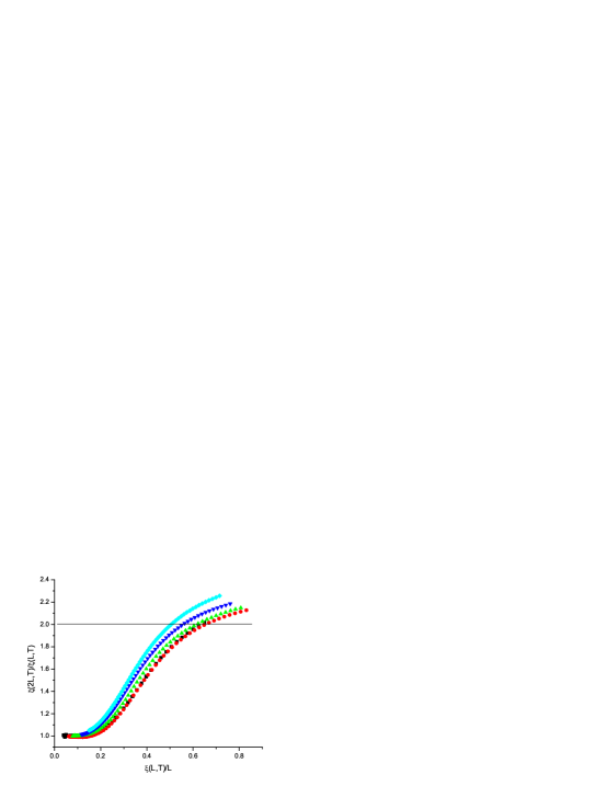
Figure 1: (Color online) Scaling plot for correlation length ratios $\xi(2L,T)/\xi(L,T)$ against $\xi(L,T)/L$ following Ref. caracciolo:95, . Top to bottom $L=3,4,6,8,12$ cyan, blue, green, red, black.

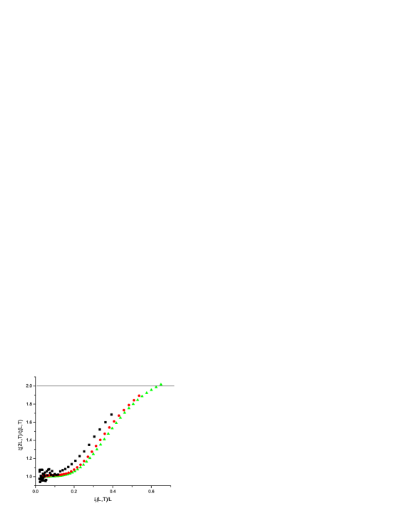
Figure 2: (Color online) Scaling plot for correlation length ratios $\xi(2L,T)/\xi(L,T)$ against $\xi(L,T)/L$ following Ref. caracciolo:95, . Top to bottom $L=24,16,12$ black, red, green.

Figure 3: (Color online) Scaling plot for reduced susceptibility ratios $\chi(2L,T)/\chi(L,T)$ against $\xi(L,T)/L$ following Ref. caracciolo:95, . Top to bottom $L=3,4,6,8,12$ : cyan, blue, green, red, black.

Figure 4: (Color online) Scaling plot for reduced susceptibility ratios $\chi(2L,T)/\chi(L,T)$ against $\xi(L,T)/L$ following Ref. caracciolo:95, . Top to bottom $L=24,16,12$ : black, red, green.

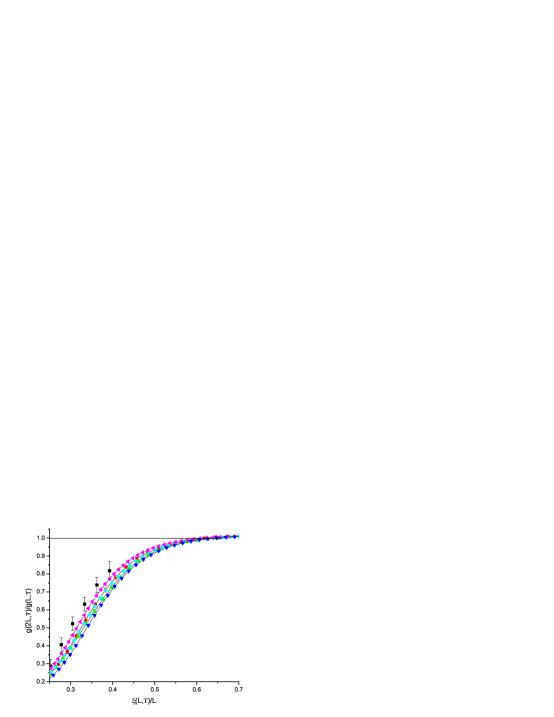
Figure 5: (Color online) Scaling plot for Binder parameter ratios $g(2L,T)/g(L,T)$ against $\xi(L,T)/L$ following Ref. caracciolo:95, . $L=24,16,12,8,6,4$ : black, red, green, blue, cyan, magenta.

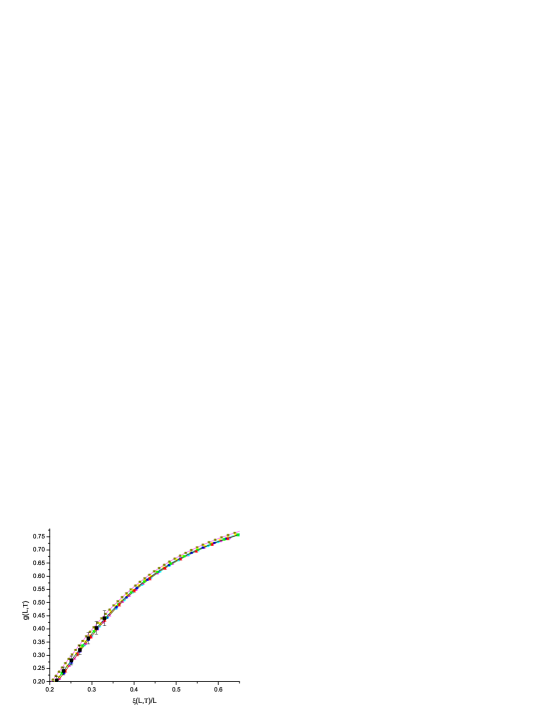
Figure 6: (Color online) Scaling plot of the Binder parameter $g(L,T)$ against $\xi(L,T)/L$. $L=48,32,24,16,12,8,6,4$ : black, red, green, blue, cyan, magenta, yellow, dark yellow.

The data were analyzed using the Caracciolo et al caracciolo:95 finite size ratio scaling approach. Figures 1 and 2 show the ratio scaling plots for the correlation length $\xi(L,T)$. In order to be able to visualize the non-monotonic behavior we present the data in two scaling plots. It can be seen that for small $L$ the scaling curves move systematically from left to right with increasing $L$; then as $L$ is increased further beyond $L\sim 24$ the curves begin to move to the left again. By inspection the present data demonstrate that in the 3D bimodal ISG there are significant finite-size corrections to scaling up to and probably beyond the largest sizes which we have studied; the observed non-monotonic behavior of the scaling plots as functions of $L$ implies that there are at least two important and conflicting correction terms. The critical normalized correlation length $(\xi(L,T)/L)_{c}$ corresponds to the $x$ coordinate of the intersection of the limiting large size curve with the horizontal line $y=2$. Data taken only up to $L\sim 24$ give the impression that the large size limit has been reached by this size, and that $(\xi(L,T)/L)_{c}\sim 0.65$ (see Katzgraber et al and Hasenbusch et al  katzgraber:06 ; hasenbusch:08 ). However when data up to larger $L$ including $L=48$ are taken into account, it is clear that one needs to go far beyond $L\sim 24$ to reach the limit where FSS corrections have become negligible; the data indicate that the true large size limit for $(\xi(L,T)/L)_{c}$ will lie below $0.65$, and will correspond to an ordering temperature $T_{c}$ in the infinite size limit significantly higher than recent estimates kawashima:96 ; ballesteros:00 ; katzgraber:06 ; hasenbusch:08 .

Figures 3 and 4 show the analogous ratio scaling plot for the SG susceptibility $\chi(L,T)$. Again for small $L$ the curves move systematically to the right with increasing $L$, and then begin to move to the left for larger $L$. Once more the position of the infinite $L$ limit curve is difficult to judge but it would correspond to a value for the exponent $\eta$ less negative than that suggested by recent estimates katzgraber:06 ; hasenbusch:08 . Figure 5 shows a ratio scaling plot for the Binder parameter $g(L,T)$. Again similar behavior can be observed. It is of interest to note that when the same data are represented in the form of a plot of $g(L,T)$ against $\xi(L,T)/L$ as in Fig. 6, for $L>4$ all the points lie on a single curve within the present statistics. This form of scaling plot is very insensitive to corrections to scaling because $g(L,T)$ and $\xi(L,T)/L$ are closely correlated.

Comparisons have been made between different spin glasses using this form of scaling plot (e.g. Ref. katzgraber:06, ) because systems lying in different universality classes should not have the same scaling curves. However simple inspection of figures 1, 2, 3 and 4 shows that $g(L,T)$ remains an almost unique function of $\xi(L,T)/L$ even when strong finite size corrections to scaling are obvious in the ratio scaling plots for each of the two parameters taken individually. In other words the corrections to scaling for $g(L,T)$ and for $\xi(L,T)/L$ are strongly correlated. Because this particular form of scaling is very insensitive to corrections, using such plots to judge if two systems lie in the same universality class or not would require data of extremely high statistical precision.

As an illustration, ratio data are shown as functions of $L$ in figures 7, 8 and 9 for one fixed normalized correlation length value, $\xi(L,T)/L=0.393$. The figures demonstrate the non-monotonic behavior, and also the difficulty in extrapolating to infinite $L$ when aiming to estimate the limiting ratio values, even at temperatures well above criticality. If nevertheless we assume that the $\xi(48,T)/\xi(24,T)$ ratio curve is close to the infinite size limit, and we extrapolate the curve to $\xi(48,T)/\xi(24,T)=2$ we obtain $T_{c}\sim 1.175$, which in view of the extrapolations we have been obliged to make can be considered as a lower limit to the true value of $T_{c}$. We recall that a quite independent “dynamic” estimate mari:01 gives $T_{c}\sim 1.19$. This value is consistent with the present equilibrium analysis.

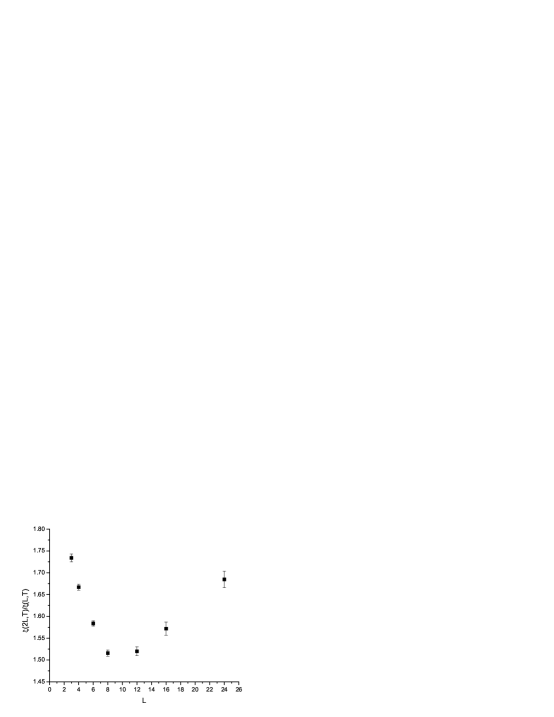
Figure 7: Correlation length ratios $\xi(2L,T)/\xi(L,T)$ against $L$ for $\xi(L,T)/L=0.393$.

Figure 8: Susceptibility ratios $\chi(2L,T)/\chi(L,T)$ against $L$ for $\xi(L,T)/L=0.393$.

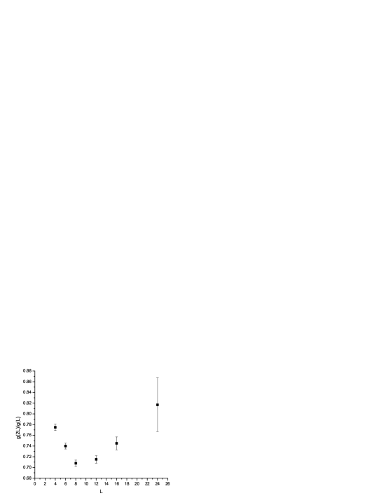
Figure 9: Binder parameter ratios $g(2L,T)/g(L,T)$ against $L$ for $\xi(L,T)/L=0.393$.

It is important to envisage potential sources of systematic error in the present data. Even though stringent precautions have been taken to assure full equilibration, as always with spin glass simulations a possible source of error which must be kept in mind would be incomplete equilibration. As stated above, the data for sizes up to $L=24$ are in very good agreement with those from reliable independent studies(Ref. katzgraber:06, and Helmut Katzgraber, private communication). It should be noted that a lack of equilibration for the larger samples only ($L=48$ and $L=32$) would reduce $\xi(2L,T)$ and $\chi(2L,T)$ for $L=24$ and $L=16$ while leaving $\xi(L,T),\chi(L,T)$ and $\xi(L,T)/L$ unaltered, and so would artificially move the scaling curves of Figures 2 and 4 downwards. The observation that the curves for $\xi(48,T)/\xi(24,T)$ and $\xi(32,T)/\xi(16,T)$ in these two figures lie well above the others thus cannot be an artifact arising from lack of equilibration at $L=48$ and $L=32$. There remain of course purely statistical sampling effects due to the fact that at large sizes the number of samples studied is necessarily restricted. For the sizes $L=48$ and $L=32$ the only data with which comparisons could be made are those from the pioneering work of Ref. palassini:99, ; these are fragmentary and recorded on far fewer samples than in the present work, but within the statistical errors there is agreement, particularly for the two $L=48$ points from $64$ samples recorded by Ref. palassini:99, .

For the 3D Gaussian ISG, corrections to scaling are much very weaker than in the bimodal case katzgraber:06 , so it can plausibly be assumed that the estimates for $T_{c}$ and for the critical values of $\xi(L,T)/L$ and $g(L,T)$ from the largest $L$ Gaussian ISG data katzgraber:06 can be taken as being essentially equal to the infinite size thermodynamic limit values. Unless strong corrections appear when still larger $L$ Gaussian samples are studied, the Gaussian critical parameters in the thermodynamic limit are not equal to those for the thermodynamic limit bimodal ISG derived as outlined above, implying that the two systems do not lie in the same universality class.

III Finite-size corrections to scaling

Clearly it is essential to allow for corrections to scaling in order to obtain reliable estimates of the critical parameters. At criticality FSS expressions including correction terms can be written as (see for instance Ref. hasenbusch:06, )

$$\chi(L,\beta_{c})=C_{\chi}L^{2-\eta}[1+a_{1}L^{-\omega}+a_{2}L^{-\omega_{2}}+\ldots]$$ (7)

where $\omega$ and $\omega_{2}$ are the first and second correction exponents. For standard ferromagnets these exponents are rather accurately known from RGT; in dimension 3 $\omega\sim 0.51$ and $\omega_{2}\sim 0.82$ in pure systems and $\omega\sim 0.3$ and $\omega_{2}\sim 0.8$  hasenbusch:06 for diluted ferromagnets. Unfortunately there are no equivalent RGT guide-lines for the values of the correction exponents (and a fortiori for the strengths of the correction terms) in ISGs. The non-monotonic variation of the positions of the scaling curves with increasing $L$ in the 3D bimodal ISG implies that there are two significant contributions (at least) with opposite signs to the finite-size-scaling corrections, coming from $\omega$ and $\omega_{2}$ terms.

For finite-size scaling with corrections near $T_{c}$, Calbrese et al  calbrese:03 give the ansatz

$$\xi(2L,T)/\xi(L,T)=F(L/\xi(L,T))+L^{-\omega}G(L/\xi(L,T))$$ (8)

and the equivalent equation for $\chi$, where $F$ and $G$ are scaling functions and $\omega$ is the leading non-analytic correction to scaling exponent. Unfortunately the present data are manifestly insufficient to attempt fits to analogous equations with two correction terms, so we can make no sensible estimate of the correction exponents in the 3D bimodal ISG.

It can be noted that in the 2d Bimodal ISG (which orders only at $T=0$) limiting behavior at criticality is only attained above $L\sim 100$ hartmann:01 .

IV Conclusion

Equilibrium numerical data on the three dimensional bimodal Ising spin glass for samples up to size $L=48$ show that corrections to finite-size scaling are unexpectedly strong and non-monotonic. Taking into account the influence of these corrections, it can be concluded that the large size limit behavior and the corresponding thermodynamic limit critical temperature and critical parameters are significantly different from the values derived from previous equilibrium simulation data where smaller maximum sizes were studied. Estimates of critical parameters from the present data are only indicative due to the intrinsic problem of extrapolating reliably to infinite size, but they are consistent with those obtained from a “dynamic” method bernardi:96 ; mari:01 ; pleimling:05 . The strong corrections to finite size scaling must be fully taken into account before a valid comparison can be made between the thermodynamic limit behaviors for the bimodal and Gaussian 3D ISGs. The data as they exist cannot be considered to show that the two systems lie in the same universality class.

- (1) S.K. Ma, Modern Theory of Critical Phenomena, (Benjamin, New York, 1976)
- (2) A. B. Harris and T. C. Lubensky, Phys. Rev. Lett. 33, 1540 (1974).
- (3) I. A. Campbell, K. Hukushima and H. Takayama, Phys. Rev. Lett. 97, 117202 (2006).
- (4) N. Kawashima and A. P. Young, Phys. Rev. B 53, R484 (1996).
- (5) H. G. Ballesteros, A. Cruz, L. A. Fernandez, V. Martin-Mayor, J. Pech, J. J. Ruiz-Lorenzo, A. Tarancon, P. Tellez, C. L. Ullod, and C. Ungil, Phys. Rev. B 62, 14237 (2000).
- (6) H. G. Katzgraber, M. Körner and A. P. Young, Phys. Rev. B 73, 224432 (2006).
- (7) M. Hasenbusch, A. Pelissetto and E. Vicari, J. Stat. Mech., L02001 (2008), Phys. Rev. B 78, 214205 (2008).
- (8) L. W. Bernardi, S. Prakash and I. A. Campbell, Phys. Rev. Lett. 77, 2801 (1996).
- (9) P. O. Mari and I. A. Campbell, arXiv:cond-mat/0111174 (2001).
- (10) M. Pleimling and I. A. Campbell, Phys. Rev. B 72, 184429 (2005).
- (11) F. Cooper, B. Freedman and D. Preston, Nucl. Phys. B 210, 210 (1982).
- (12) R. Fisch and A. B. Harris, Phys.Rev.Lett. 38, 785 (1977).
- (13) R. R. P. Singh and S. Chakravarty, Phys.Rev.Lett. 57, 245 (1986).
- (14) L. Klein, J. Adler, A. Aharony, A. B. Harris and Y. Meir, Phys.Rev.B 13, 11249 (1991).
- (15) D. Daboul, I. Chang and A. Aharony, Euro. Phys. J. B 41, 231 (2004).
- (16) S. Caracciolo, R. G. Edwards, S. J. Ferreira, A. Pelissetto and A. D. Sokal, Phys.Rev.Lett. 74, 2969 (1995).
- (17) M. Palassini and S. Caracciolo, Phys. Rev. Lett. 82, 5128 (1999).
- (18) K. Hukushima and K. Nemoto, J. Phys. Soc. Jpn. 65, 1604 (1996).
- (19) M. Hasenbusch, F. Parisen Toldin, A. Pelissetto, and E. Vicari, J.Stat.Mech., P02016 (2007).
- (20) P. Calbrese, V. Martín Mayor, A. Pelissetto and E. Vicari, Phys.Rev.B 68, 036136 (2003).
- (21) A. K. Hartmann and A. P. Young, Phys. Rev. B 64, 180404 (2001).
- (22) D. A. Huse, Phys. Rev. B 40, 304 (1989).
- (23) M. Hasenbusch, A. Pelissetto, and E. Vicari, J. Stat. Mech., P11009 (2007).
- (24) T. Nakamura, arXiv:cond-mat/0603062.
- (25) A. T. Ogielski, Phys. Rev. B 32, 7384 (1985).
- (26) H. Reiger, J. Phys. A 26, L615 (1993).
- (27) H. G. Katzgraber and I. A. Campbell, Phys. Rev. B 72, 014462 (2005).