General theory for integer-type algorithm
for higher order differential equations

Abstract

Based on functional analysis, we propose an algorithm for finite-norm solutions of higher-order linear Fuchsian-type ordinary differential equations (ODEs) $P(x,\frac{d}{dx})f(x)=0$ with $P(x,\frac{d}{dx}):=\displaystyle\Bigl{(}\sum_{m=0}^{M}p_{m}(x)\bigl{(}{\textstyle\frac{d}{dx}}\bigr{)}^{m}\Bigr{)}$ by using only the four arithmetical operations on integers.

This algorithm is based on a band-diagonal matrix representation of the differential operator $P(x,\frac{d}{dx})$, though it is quite different from the usual Galerkin methods. This representation is made for the respective CONSs of the input Hilbert space ${\cal H}$ and the output Hilbert space ${{\cal H}^{\Diamond}}$ of $P(x,\frac{d}{dx})$. This band-diagonal matrix enables the construction of a recursive algorithm for solving the ODE. However, a solution of the simultaneous linear equations represented by this matrix does not necessarily correspond to the true solution of ODE. We show that when this solution is an $\ell^{2}$ sequence, it corresponds to the true solution of ODE. We invent a method based on an integer-type algorithm for extracting only $\ell^{2}$ components. Further, the concrete choice of Hilbert spaces ${\cal H}$ and ${{\cal H}^{\Diamond}}$ is also given for our algorithm when $p_{m}$ is a polynomial or a rational function with rational coefficients. We check how our algorithm works based on several numerical demonstrations related to special functions, where the results show that the accuracy of our method is extremely high.

Keywords

higher-order linear ODE, rational-type smooth basis function, integer-type algorithm, band-diagonal matrix, eigenfunction, numerical analysis, high accuracy.

AMS: 65L99, 42C15, 65L60, 34A45

1 Introduction

Linear ordinary differential equations (ODE) of the type

$$P(x,{\textstyle\frac{d}{dx}})f(x):=\left(\sum_{m=0}^{M}p_{m}(x)\left(\frac{d}{dx}\right)^{m}\right)f(x)=0$$ (1)

are very important tools in many fields (physics, engineering etc.). In many useful cases, the functions $p_{m}(x)$ are polynomials or rational functions. As is well known, it is difficult in general to solve them analytically for higher-order cases although there are relatively general methods for second-order equations with low-degree polynomials $p_{m}(x)$, for which we employ hypergeometric functions (or special functions) [2] and power series expansions about nonsingular points or regular singular points [1]. (Practically, instead of analytical methods, many kinds of numerical methods have been proposed and used.) The aim of this paper is to obtain solutions $f(x)$ of a linear ODE (1) in a Hilbert space ${\cal H}$ of functions on $\mathbb{R}$ when the equation is of higher order and/or the function $p_{m}(x)$ is of higher degree. Solutions with finite norm are sometimes very important in quantum mechanics (e.g. wavefunctions of particles bound by potentials) [3], and for transit or temporary phenomena in signal processing and circuit theory that are almost localized in the time coordinate in many applications, for example.

In this paper, we propose an integer-type general algorithm for solving these ODEs, by choosing function spaces and their basis systems appropriately. This method is based on a pair of Hilbert spaces ${\cal H}$ and ${{\cal H}^{\Diamond}}$ with distinct inner products, where the domain of the differential operator $P(x,{\textstyle\frac{d}{dx}})$ is a dense subspace of ${\cal H}$ and its range is a subspace of ${{\cal H}^{\Diamond}}$. Under appropriate choice of these spaces and their basis systems which will be presented in this paper, a differential equation can be expressed by band-diagonal-type simultaneous linear equations, and all the ‘matrix elements’ are rational-(complex-)valued. Moreover, under the same choice, all the basis functions are rational functions. In addition, from the properties of the basis functions used, this method has a somewhat similar feature to power series expansions about nonsingular points or regular singular points, in the sense that the solution can be expanded as linear combinations of the powers of a rational function of $x$ with rational coefficients. From another point of view, this method is closely related to the Laurent expansion and hyperfunctions in complex analysis and to the Fourier series, under some changes of variable. Therefore, this method has a ‘semi-analytical’ character and it can be discussed from the standpoint of mathematical analysis, though it is a kind of numerical method.

Since it is difficult to apply analytical methods to general higher-order linear differential equations, various kinds of numerical methods have been proposed. One group is based on the discretization of coordinate or on the differences or on the relations between adjacent lattice points (Runge-Kutta methods, for example). Another group is based on finite-dimensional subspaces of an infinite-dimensional function space, such as the collocation method, the Ritz-Galerkin method and the Petrov-Galerkin method [4] [5], for example. In this group, many kinds of finite element methods [5] [6] have been proposed and used widely and efficiently in many fields. These methods construct subspaces spanned by finite elements with very localized compact supports. In addition, this group contains a subgroup which uses subspaces spanned by globally smooth basis functions [4] such as the Hermite functions.

The method to be proposed in this paper is similar to the latter subgroup in the sense that it is based on the finite-dimensional subspaces spanned by global smooth basis functions.

The proposed method is different from Ritz-Galerkin method, in that the function space ${{\cal H}^{\Diamond}}$ is different from ${\cal H}$, and ${{\cal H}^{\Diamond}}$ is wider than ${\cal H}$ in the proposed method. Here, remember that the function space ${\cal H}$ corresponds to the domain of the differential operator $P(x,{\textstyle\frac{d}{dx}})$ and the function space ${{\cal H}^{\Diamond}}$ does to the range of $P(x,{\textstyle\frac{d}{dx}})$. The choice of different function spaces ${\cal H}$ and ${{\cal H}^{\Diamond}}$ may be possible even for Petrov-Galerkin method. However, the method proposed here is quite different from the usual ‘standard truncation methods’ or ‘projection methods’ such as the Ritz-Galerkin and Petrov-Galerkin methods, in respect of the following point:

Although the Ritz-Galerkin and Petrov-Galerkin methods are based on the solutions of simultaneous linear equations with a square matrix truncated within a finite dimension, the method proposed here is based on finite-dimensional truncations of the exact solutions of the infinite-dimensional simultaneous linear equations. There is a possibility that our numerical solution coincides exactly with the orthogonal projection of the true solution to the finite-dimensional subspace, whatever its dimension may be, and we have already had some numerical examples where this perfect coincidence occurs really [7]. In order to realize this direction, we solve simultaneous linear equations with a non-square-type band-diagonal matrix, in which its column is larger than its row. Since the solution is not unique because this non-square-type band-diagonal matrix has a non-trivial kernel, we have to extract one solution among the above solutions. In order to resolve this problem, we extract one solution among them using a novel method, which will be explained in the latter part of this introduction. Further, this matrix elements do not change when the dimension of the subspace increases. Hence the proposed method provides a recursive algorithm with no round-off errors up to an arbitrary dimension for the vectors of the space of exact solutions of the infinite-dimensional simultaneous linear equations.

The method to be proposed has five advantages other than the integer-type property mentioned above, as follows; (1) especially when the ODE has no singular point or when the ODE belongs to the Fuchsian class even if it has singular points, this method can determine the structure itself of the function space of solutions in ${\cal H}$ of the differential equation, directly from the numerical results. (2) Another advantage is that the convergence of the error to $0$ is guaranteed as the dimension of the subspace tends to infinity, and an upper bound of the error can be given for the finite-dimensional case. (3) Moreover, it does not require any calculation of large matrices (inverse matrix, eigenvector, etc.) for solving our simultaneous linear equations. (4) Another strong point is that the basis functions of ${\cal H}$ are smooth sinusoidal-like wavepackets with spindle-shaped envelopes, which are suitable for the expansion of various kind of ‘natural’ functions decaying as $x\to\pm\infty$. In this sense, the basis functions contain both global and local information. (5) Another strong point is that this method requires a small amount of calculations for obtaining high-accuracy solutions. For example, when the coefficients in the expansion of a true solution by the basis functions decay exponentially, the amount of calculations required by this method is almost proportional asymptotically to the cube of the number of required significant digits.

In this paper, we will show the validity of the band-diagonal matrix representation, i.e., we will show that the square-summable solutions of the simultaneous linear equations according to the band-diagonal matrix always correspond to true solutions of the ODE except at the singular points of the ODE. Especially, when the ODE has no singular point, we will show the one-to-one correspondence between the true solutions in ${\cal H}$ of the differential equation and the square-summable number sequences satisfying the simultaneous linear equations represented by the band-diagonal matrix. The larger part of its proofs is based mainly on functional analysis. Similar one-to-one correspondence can be proved for the cases of the Fuchsian class by a modification even if the ODE has singular points.

However, the presented method has a pitfall based on finite-dimensional truncations of the exact solutions of the infinite-dimensional simultaneous linear equations. This pitfall is due to the non-uniqueness of non-square-summable solutions of the simultaneous linear equations because the number of linearly independent solutions of the simultaneous linear equation is not smaller than the bandwidth whereas the number of linearly independent solutions of the differential equations is not greater than its order $M$. That is, there are solutions which do not correspond to true solutions of the differential equations, we call these solutions extra solutions. In order to resolve this problem, we propose a method to to remove the extra solutions effectively. This method is based on quasi-minimization of the ratio between a norm sensitive to divergence and another norm insensitive to divergence. This quasi-minimization guarantees the convergence to $0$ of the error in the numerical results; the accuracy of the numerical results is sufficiently high, even for finite dimensions.

For minimization of the ratio between two quadratic forms, the usual method is based on the eigenspace of the matrix $A^{-\frac{1}{2}}BA^{-\frac{1}{2}}$ with the two corresponding inner-product-matrices $A$ and $B$. However, it is difficult to apply this method to the above problem, due to round-off errors, because these inner-product matrices are usually very close to a singular matrix with rank $1$. However, in this paper, we propose an alternative integer-type method for quasi-minimization, which does not require as much calculation as the usual method. This method is based on a kind of quasi-orthogonalization of integer-valued vectors, which is realized by an idea that is conceptually between the Gram-Schmidt process and the Euclidean algorithm.

An integer-type recursive algorithm similar to the proposed one may be applied also to the Petrov-Galerkin method, in order to calculate the head and intermediate rows of solution vectors of the system of simultaneous linear equations described by a large-dimensional band-diagonal square matrix. However, in this case, we have to calculate new linear combinations of solution vectors satisfying the final constraints (linear equations in the bottom rows). For this calculation, we can solve another system of simultaneous linear equations, which is described by another square matrix whose dimension is half a band width. However, this matrix is usually very close to a singular matrix of rank 1. Moreover, the elements in the bottom rows of the solution vectors are rational numbers whose numerators and denominators are huge integers. Therefore, this type of Petrov-Galerkin method requires a much larger amount of calculations than the proposed method based on non-square matrix and integer-type quasi-orthogonalization.

Table 1: Difference from Galerkin methods for norm-finite solutions (without initial conditions)

Method	Ritz-Galerkin	Petrov-Galerkin	proposed
${{\cal H}^{\Diamond}}$ and ${\cal H}$	same	same/different	different
Corresponding matrix	square		non-square and
with truncation	(band-diagonal / general)		band-diagonal
Extra solutions	No		can be removed
	Eigenvalue and eigenvector		Exact kernel vector
Solution vector	of finite-dimensional matrix		(infinite-dimensional)

The contents of the paper are as follows; Section 2 explains an abstract framework for a general algorithm, using a pair of Hilbert spaces ${\cal H}$ and ${{\cal H}^{\Diamond}}$ with distinct inner products. Subsection 2.1 states the basic conditions for the pair of Hilbert spaces ${\cal H}$ and ${{\cal H}^{\Diamond}}$. This subsection gives a sufficient condition for band-diagonal matrix representation for the ODE. In Subsection 2.2, using this band-diagonal form, we provide the basic structure of our recursive algorithm with removal of non-$\ell^{2}$-components. Section 3 presents the concrete choices of Hilbert spaces and basis systems used in our algorithm, and checks that they satisfy the conditions given in Section 2. Section 4 gives proofs of theorems mentioned in Section 2. In Section 5, we give some numerical examples related to special functions and show how effectively our algorithm works, where we are successful to solve ODEs in a very high accuracy with a relatively small amount of calculations (approximately proportional to a power of the number of required significant digits, empirically). Moreover, we show how numerical results are successful even for the cases with singular points. Section 6 discusses a related topic and further extensions of our algorithm.

2 Abstract structure of our algorithm

Table 2: Components of our algorithm

$P(x,{\textstyle\frac{d}{dx}})$	Differential operator	Top of 2.1
$M$	Order of $P(x,{\textstyle\frac{d}{dx}})$	Top of 2.1
$p_{m}(x)$	Polynomial: $m$-th order coefficient func. of $P(x,{\textstyle\frac{d}{dx}})$	Top of 2.1
${\cal H}$	Input Hilbert space	Top of 2.1
${{\cal H}^{\Diamond}}$	Output Hilbert space	Top of 2.1
$\tilde{A}_{P}$	Operator ${\cal H}\to{\cal H}$ defined as action of $P(x,\frac{d}{dx})$	Top of 2.1
$A_{P}$	Closed extension of $\tilde{A}_{P}$	Top of 2.1
$\tilde{B}_{P}$	Operator ${\cal H}\to{{\cal H}^{\Diamond}}$ defined as action of $P(x,\frac{d}{dx})$	Top of 2.1
$B_{P}$	Closed extension of $\tilde{B}_{P}$	Top of 2.1
$e_{n}$	Basis of ${\cal H}$	C1
$e_{n}^{\Diamond}$	Basis of ${\cal H}^{\Diamond}$	C1
$f_{n}$	$f_{n}:=\langle f,e_{n}\rangle_{{{\cal H}}}$ for $f\in{\cal H}$	Theorem 2.1
$\vec{f}$	Vector representation of $\{f_{n}\}_{n=0}^{\infty}$	after (4)
$b_{m}^{n}$	Matrix element for $B_{P}$: $b_{m}^{n}:=\langle B_{P}e_{n},e_{m}^{\Diamond}\rangle_{{{\cal H}^{\Diamond}}}$	C2
$\ell_{0}$	Bandwidth parameter: $b_{m}^{n}=0$ for $|m-n|>\ell_{0}$	C2
$j_{0}$	Integer s.t. $b_{m}^{m+\ell_{0}}\neq 0$ for any integer $m\geq j_{0}$	C5
$N$	Dimension of subspace where recursion is executed	C7 and Algorithm
$K$	Dimension of subspace of final approximate solutions	C7 and Algorithm
$D$	Dimension of solution space of $\sum_{m}b_{m}^{n}f_{n}=0$	after (6)
$p_{0}$	Integer $p_{0}:=j_{0}+\ell_{0}-1$	after (6)
$\|\cdot\|_{\ell^{2},K}$	‘Truncated norm’ for number sequences	(15)

2.1 General framework for general linear ordinary differential equation

In this paper, we consider a general linear ordinary differential equation given by the differential operator $P(x,{\textstyle\frac{d}{dx}})$ defined on the space of $M$-times differentiable functions $C^{M}(\mathbb{R})$:

$$P(x,{\textstyle\frac{d}{dx}})f=0,$$ (2)

where $M$ is the order of the differential operator $P(x,{\textstyle\frac{d}{dx}})$. The main purpose of this paper is to analyze the structure of the solution space of (2) on a given Hilbert space ${\cal H}$ that densely contains $C^{M}(\mathbb{R})$. For this purpose, we define the operator $\tilde{A}_{P}$ as the action of the differential operator $P(x,{\textstyle\frac{d}{dx}})$ with domain

$$D(\tilde{A}_{P}):=\{f\in C^{M}(\mathbb{R})\cap{\cal H}|P(x,{\textstyle\frac{d}{dx}})f\in{\cal H}\}.$$

Then, the linear operator $A_{P}$ is given as the closed extension of $\tilde{A}_{P}$ with respect to the graph norm  [10]. That is, we treat the structure of the solution space of the differential equation:

$$A_{P}f=0.$$

The main goal is to construct an integer-type numerical algorithm for finding non-zero solutions of the differential equation given by the differential operator $A_{P}$ when the original space ${\cal H}$ is contained in a larger Hilbert space ${{\cal H}^{\Diamond}}$ as a set. Here, the larger Hilbert space ${{\cal H}^{\Diamond}}$ also densely contains $C^{M}(\mathbb{R})$. For this purpose, we construct a band-diagonal matrix representation of the differential operator $A_{P}$ under certain conditions. In order to obtain a band-diagonal matrix representation, we introduce a linear operator $B_{P}$ from a dense subspace of ${\cal H}$ to ${{\cal H}^{\Diamond}}$, which is defined as the closed extension of $\tilde{B}_{P}$ with respect to the graph norm of the operator $\tilde{B}_{P}$ defined by the action of the differential operator $P(x,{\textstyle\frac{d}{dx}})$ with the following domain:

$$D(\tilde{B}_{P}):=\{f\in C^{M}(\mathbb{R})\cap{\cal H}|P(x,{\textstyle\frac{d}{dx}})f\in{{\cal H}^{\Diamond}}\}.$$

In order to using a band-diagonal structure, we introduce three conditions for the quintuplet consisting of the linear differential operator $P(x,{\textstyle\frac{d}{dx}})$, the Hilbert spaces ${\cal H}$ and ${{\cal H}^{\Diamond}}$, and their CONSs $\{e_{n}\,\}_{n=0}^{\infty}$ and $\{e_{n}^{\Diamond}\}_{n=0}^{\infty}$, which is abbreviated to $(P(x,{\textstyle\frac{d}{dx}}),{\cal H},\{e_{n}\,\}_{n=0}^{\infty},{{\cal H}^{\Diamond}},\{e_{n}^{\Diamond}\}_{n=0}^{\infty})$. These conditions are shown to hold in several examples for $P(x,{\textstyle\frac{d}{dx}})$ later. In what follows, $\langle\cdot,\,\cdot\rangle_{{{\cal H}^{\Diamond}}}$ and $\langle\cdot,\,\cdot\rangle_{{\cal H}}$ denote the inner products of ${{\cal H}^{\Diamond}}$ and ${\cal H}$ respectively.

C1

For any $n$, $e_{n}$ belongs to $D(\tilde{B}_{P})$.

C2

There exists an integer $\ell_{0}$ such that $b_{m}^{n}:=\langle B_{P}e_{n},e_{m}^{\Diamond}\rangle_{{{\cal H}^{\Diamond}}}=0$ when $|n-m|>\ell_{0}$.

C3

There exists a linear operator $C_{P}$ with domain $D(C_{P})$ from a dense subspace of ${{\cal H}^{\Diamond}}$ to ${\cal H}$ such that $e_{m}^{\Diamond}\in D(C_{P})$ and $\langle B_{P}f,e_{m}^{\Diamond}\rangle_{{{\cal H}^{\Diamond}}}=\langle f,C_{P}e_{m}^{\Diamond}\rangle_{{\cal H}}$ for $f\in D(\tilde{B}_{P})$.

Due to Condition C3, the basis $e_{m}^{\Diamond}$ belongs to the domain of the adjoint operator $B_{P}^{*}$. Under these conditions, we obtain the following.

Proposition 2.1

A function $f$ of the kernel of $A_{P}$ belongs to the kernel of $B_{P}$.

This proposition is immediate from the fact that the domain of $B_{P}$ includes the domain of $A_{P}$.

Theorem 2.1

Assume that the quintuplet $(P(x,{\textstyle\frac{d}{dx}}),{\cal H},\{e_{n}\,\}_{n=0}^{\infty},{{\cal H}^{\Diamond}},\{e_{n}^{\Diamond}\}_{n=0}^{\infty})$ satisfies Conditions C1 - C3. For any function $f$ of the kernel of $B_{P}$ and any $m\in\mathbb{Z}^{+}$, the $\ell^{2}$-sequence $\{f_{n}:=\langle f,e_{n}\rangle_{{\cal H}}\}_{n=0}^{\infty}$ satisfies

$$\sum_{n=\max(0,\,m-\ell_{0})}^{m+\ell_{0}}b_{m}^{n}f_{n}=0,$$ (3)

i.e., belongs to the linear space

$$V := \bigl{\{}\vec{f}:=\{f_{n}\}_{n=0}^{\infty}\,\,\bigl{|}\,\sum_{n=0}^{\infty}b_{m}^{n}f_{n}=0\,\,\,(m\in\mathbb{Z}^{+})\,\bigr{\}}$$ (4)

$$= \bigl{\{}\vec{f}\,\,\bigl{|}\,\!\!\!\!\!\sum_{n=\max(0,m-\ell_{0})}^{m+\ell_{0}}\!\!\!\!\!b_{m}^{n}f_{n}=0\,\,\,(m\in\mathbb{Z}^{+})\,\bigr{\}}.$$

The proof of this theorem will be given in Subsection 4.1 of this section. Due to Condition C2, the dimension of $V$ is finite.

However, square-summable number sequences satisfying (3) do not always correspond to functions in the domain of $A_{P}$ (hence in the kernel of $A_{P}$). When the linear ordinary differential equation (2) has singular points, i.e., its solution has singular points, we denote the set of the singular points by $S$. In this case, the obtained solutions do not necessarily belong to $C^{M}(\mathbb{R})$, but they belongs to $C^{M}(\mathbb{R}\setminus S)$ under some conditions. So, ${\cal H}$ has to include the space $C^{M}(\mathbb{R}\setminus S)$. In order to guarantee that the obtained solutions are true solutions, we require another condition:

C4

For any sequence $\{f_{n}\}_{n=0}^{\infty}\in V\cap\ell^{2}(\mathbb{Z}^{+})$, the sum $\displaystyle\sum_{n=0}^{N}f_{n}e_{n}$ converges to a solution $f\in C^{M}(\mathbb{R}\setminus S)\cap{\cal H}$ of $P(x,\frac{d}{dx})f=0$ as $N\to\infty$ for ${\cal H}$-norm.

Therefore, if the above condition holds, any a square-summable kernel vector of the band-diagonal matrix $b_{m}^{n}$ gives a solution of ODE (2) in $C^{M}(\mathbb{R}\setminus S)\cap{\cal H}$. In the remainder of this paper, we often use this vector representation instead of a number sequence, for simplicity.

In the non-singular case, the following theorem holds.

Theorem 2.2

Assume two assumptions: (1) the linear ordinary differential equation (2) has no singular points. (2) the quintuplet $(P(x,{\textstyle\frac{d}{dx}}),{\cal H},\{e_{n}\,\}_{n=0}^{\infty},{{\cal H}^{\Diamond}},\{e_{n}^{\Diamond}\}_{n=0}^{\infty})$ satisfies Conditions C1-C4. Then, the map $f\mapsto\{\langle f,e_{n}\rangle_{{\cal H}}\}_{n=0}^{\infty}$ provides a one-to-one correspondence between the $\ell^{2}$-solutions of (3) and the solutions in $C^{M}(\mathbb{R})\cap{\cal H}$ of (2).

The proof is directly derived from Theorem 2.1 and Condition C4 itself as follows. When a function $f$ in $C^{M}(\mathbb{R})\cap{\cal H}$ satisfies the differential equation (2), it belongs to $D(\tilde{A}_{P})\,(\subset D(A_{P}))$ and satisfies $A_{P}f=0$. Then, Theorem 2.1 and Lemma 2.1 guarantee that $\{\langle f,e_{n}\rangle_{{\cal H}}\}_{n=0}^{\infty}$ belongs to $V\cap\ell^{2}(\mathbb{Z}^{+})$. The reverse argument is immediate from Condition C4.

By means of Theorem 2.2, under C1-C4, the linear differential equation is reduced to the simultaneous linear equations (3) with a ‘band-diagonal structure’ of bandwidth $2\ell_{0}+1$. That is, under these conditions, the problem of finding the solutions in $C^{M}(\mathbb{R})\cap{\cal H}$ of the differential equation $P(x,{\textstyle\frac{d}{dx}})f=0$ is equivalent to the problem of finding vectors in the space $V\cap\ell^{2}(\mathbb{Z}^{+})$.

Even if the linear ordinary differential equation (2) has singular points, we have a modification of Theorem 2.2 if the differential equation (2) is Fuchsian, whose definition is given as follows.

Definition 2.1

An ODE $P(x,\frac{d}{dx})f(x):=\displaystyle\sum_{m=0}^{M}p_{m}(x)(\textstyle\frac{d}{dx})^{m}f(x)=0$ with analytic functions $p_{m}(x)$ $(m=0,1,\ldots M)$ is called Fuchsian if all of its singular points are regular singular points [1] [11] [12]. In this case, the differential operator $P(x,\frac{d}{dx})$ is called Fuchsian.

Further, in the following, a singular point of ODE $P(x,\frac{d}{dx})f(x)=0$ is called a singular point of the differential operator $P(x,\frac{d}{dx})$.

As is well known [11] [12], Fuchsian ODEs satisfy the following lemmata:

Lemma 2.1

Assume that a Fuchsian ODE $\displaystyle\sum_{m=0}^{M}p_{m}(x)(\textstyle\frac{d}{dx})^{m}f(x)=0$ with analytic functions $p_{m}(x)$ $(m=0,1,\ldots M)$ has singular points $z_{1},z_{2},\ldots z_{N}$. Then, the functions $\displaystyle\prod_{n=1}^{N}(x-z_{n})^{M-m}\,\frac{p_{m}(x)}{p_{M}(x)}$ $(m=0,1,\ldots M-1)$ are holomorphic at $z_{1},z_{2},\ldots z_{N_{1}}$.

Lemma 2.2

Assume that a Fuchsian ODE $\displaystyle\sum_{m=0}^{M}p_{m}(x)(\textstyle\frac{d}{dx})^{m}f(x)=0$ has holomorphic coefficient functions $p_{m}(x)$ $(m=0,1,\ldots M)$ on $\mathbb{R}$. Then, the set $S$ of its singular points is given by $p_{M}^{-1}(0)$.

As a corollary, we obtain the following:

Corollary 2.1

Assume that a differential operator $Q(x,\frac{d}{dx}):=\displaystyle\sum_{m=0}^{M}q_{m}(x)(\textstyle\frac{d}{dx})^{m}$ with analytic functions $q_{m}(x)$ $(m=0,1,\ldots M)$ has singular points $z_{1},z_{2},\ldots z_{N}$ and all of zero points of the coefficient function $q_{M}(x)$ are $z_{1},z_{2},\ldots z_{N}$ whose multiplicity are not smaller than $M$. Moreover, assume that the ODE $Q(x,\frac{d}{dx})f=0$ is Fuchsian. Then, there exist holomorphic functions $\tilde{q}_{m}(x)$ $(m=0,1,\ldots M-1)$ on $\mathbb{R}$ such that $\displaystyle q_{m}(x)=\tilde{q}_{m}(x)\prod_{n=0}^{N_{1}}(x-z_{n})^{m}$ and the set $S$ of its singular points is given by $q_{M}^{-1}(0)$.

We additionally assume the conditions:

C1⁺

There exists a positive function $\upsilon$ in $C^{M}(\mathbb{R})$ s.t. $\displaystyle\langle f,g\rangle_{\cal H}=\int_{-\infty}^{\infty}\!\!\!f(x)\overline{g(x)}\upsilon(x)dx$.

C2⁺

There exists a positive function ${\upsilon^{\Diamond}}$ in $C^{M}(\mathbb{R})$ s.t. $\displaystyle\langle f,g\rangle_{{\cal H}^{\Diamond}}=\int_{-\infty}^{\infty}\!\!\!f(x)\overline{g(x)}{\upsilon^{\Diamond}}(x)dx$.

When Condition C1⁺ holds, ${\cal H}$ always includes the space $C^{M}(\mathbb{R}\setminus S)$ because the set $S$ has zero measure. Now, Theorem 2.2 can be replaced by the following theorem:

Theorem 2.3

Let $Q(x,{\textstyle\frac{d}{dx}})$ be the Fuchsian differential operator satisfying the conditions of Corollary 2.1. When the quintuplet $(Q(x,{\textstyle\frac{d}{dx}}),{\cal H},\{e_{n}\,\}_{n=0}^{\infty},{{\cal H}^{\Diamond}},\{e_{n}^{\Diamond}\}_{n=0}^{\infty})$ satisfies Conditions C1-C4, C1⁺, and C2⁺, the map $f\mapsto\{\langle f,e_{n}\rangle_{{\cal H}}\}_{n=0}^{\infty}$ provides a one-to-one correspondence between the $\ell^{2}$-solutions of (3) and the solutions in $C^{M}(\mathbb{R}\setminus S)\cap{\cal H}$ of (2) concerning $B_{Q}$.

Hence, when the given conditions hold, in order to solve the Fuchsian linear ODE, it is sufficient to extract the subspace $V\cap\ell^{2}(\mathbb{Z}^{+})$ as well as in the non-singular case.

However, a general Fuchsian differential operator $P(x,{\textstyle\frac{d}{dx}}):=\displaystyle\sum_{m=0}^{M}p_{m}(x)(\textstyle\frac{d}{dx})^{m}$ does not necessarily satisfy the above condition. In this case, Theorem 2.3 can be applied in the following way. Assume that all coefficient functions $p_{m}(x)$ $(m=0,1,\ldots M)$ are holomorphic and $p_{M}(x)$ has zero points $z_{1},\ldots,z_{N}\in S$ with the multiplicity $\mu_{1},\ldots,\mu_{N}$, respectively. Then, Lemma 2.1 guarantees the inequality $\mu_{n}\leq M$. Then, the differential operator

$$Q(x,\frac{d}{dx}):=\displaystyle\prod_{n}(x-z_{n})^{M-\mu_{n}}P(x,\frac{d}{dx})$$ (5)

is Fuchsian and satifies the conditions of Corollary 2.1. So, we can apply Theorem 2.3 to the differential operator $Q(x,\frac{d}{dx})$ in stead of $P(x,\frac{d}{dx})$.

Since Condition C4 is assumed in Theorem 2.3, it is sufficient to show the following theorem, which will be shown in Subsection 4.2. That is, the combination of C4 and Theorems 2.1 and 2.4 yields Theorem 2.3.

Theorem 2.4

Let $Q(x,{\textstyle\frac{d}{dx}})$ be the Fuchsian differential operator satisfying the conditions of Corollary 2.1. Assume that the quintuplet $(Q(x,{\textstyle\frac{d}{dx}}),{\cal H},\{e_{n}\,\}_{n=0}^{\infty},{{\cal H}^{\Diamond}},\{e_{n}^{\Diamond}\}_{n=0}^{\infty})$ satisfies Conditions C1-C3, C1⁺, and C2⁺. Then, the solutions in $C^{M}(\mathbb{R}\setminus S)\cap{\cal H}$ of (2) always give functions of the kernel of $B_{Q}$.

In this theorem, the condition for the multiplicity of zero points is crucial because it is needed to expand the domain $D(B_{Q})$ sufficiently.

Remark 2.1

In general, the inner product $\langle\cdot,\,\cdot\rangle_{{\cal H}}$ of ${\cal H}$ does not coincide with the restriction on ${\cal H}$ of the inner product $\langle\cdot,\,\cdot\rangle_{{{\cal H}^{\Diamond}}}$ of ${{\cal H}^{\Diamond}}$. Further, $e_{n}^{\Diamond}$ does not necessarily belong to the domain $D(A_{P}^{*})$. In order to characterize Condition C3, we consider the special case when ${{\cal H}^{\Diamond}}={\cal H}$, $e_{n}=e_{n}^{\Diamond}$, and $\langle A_{P}e_{n},e_{m}\rangle_{{{\cal H}^{\Diamond}}}=\overline{\langle A_{P}e_{m},e_{n}\rangle_{{{\cal H}^{\Diamond}}}}$. Note that the condition ${{\cal H}^{\Diamond}}={\cal H}$ implies that $A_{P}=B_{P}$. In this case, if the operator $A_{P}$ is symmetric, Condition C3 holds. In other words, if the operator $A_{P}$ is not symmetric, Condition C3 does not necessarily hold. In such a case, if we define another linear operator $\tilde{A}_{P}^{\prime}$ whose domain is the linear expansion of $\{e_{n}\}$, its closed extension $A_{P}^{\prime}$ is symmetric, and the solution function of $A_{P}^{\prime}f=0$ satisfies the simultaneous linear equations (3). That is, if a general non-zero solution function of $A_{P}f=0$ does not belong to the domain of $A_{P}^{\prime}$, this solution does not necessarily satisfy (3). Later, in Remark 3.1, we give an example of the latter case.

The remaining tasks are divided into two parts: The first part concerns the general theory for our algorithm for solving a linear ordinary differential equation based on several conditions. This part is called general theory part. The second part concerns how to apply the above general theory for several wide classes of linear ordinary differential equations. This part is called application part.

General part

Task 1

(Subsection 2.2) Giving a recursive algorithm for band-diagonal-type simultaneous linear equations under Conditions C1-C4. This algorithm requires additional condition C5, which will be given in Subsection 2.2. The additional explanation for this algorithm is given in Subsection 2.3.

Task 2

(Subsection 2.3) Giving an integer-type algorithm realizing the above algorithm by adding Condition C6.

Task 3

(Subsection 4.1) Proof of Theorem 2.1: Showing that any $C^{M}(\mathbb{R})$ solution corresponds to an element of $V$.

Task 4

(Subsection 4.2) Proof of Theorem 2.4: Showing the one-to-one correspondence between $V\cap\ell^{2}(\mathbb{Z}^{+})$ and $C^{M}(\mathbb{R}\setminus S)\cap{\cal H}$ with the Fuchsian differential operator $Q$ given in (5).

Task 5

(Subsections 4.3) Showing the convergence of the algorithm given in Task 1.

Task 6

(Subsections 4.4) Showing that all of $\ell^{2}$ components in $V$ can be extracted by the algorithm given in Task 1 with additional condition.

Application part

Task 7

(Subsections 3.1-3.4) Constructing ${\cal H}$, ${{\cal H}^{\Diamond}}$, and their CONSs satisfying Conditions C1-C6, C1⁺, and C2⁺ for a differential operator $P(x,\frac{d}{dx})$ with polynomial coefficient functions $p_{m}(x)$.

Task 8

(Subsection 3.5) Explaining how to apply the above method to a differential operator $R(x,\frac{d}{dx})$ with rational coefficient functions $r_{m}(x)$.

In order to apply our method to a Fuchsian linear ODE $P(x,\frac{d}{dx})f=0$ with polynomial coefficient functions, it is enough to construct ${\cal H}$, ${{\cal H}^{\Diamond}}$, and their CONSs satisfying Conditions C1-C6, C1⁺, and C2⁺ with the Fuchsian linear differential operator $Q(x,\frac{d}{dx})$ given in (5). Since the Fuchsian linear differential operator $Q(x,\frac{d}{dx})$ has polynomial coefficient functions, we can apply Task 7 with replacing $P(x,\frac{d}{dx})$ by $Q(x,\frac{d}{dx})$. Due to Theorem 2.3, any solution of $P(x,\frac{d}{dx})f(x)=0$ in $C^{M}(\mathbb{R}\setminus p_{M}^{-1}(0))\cap{\cal H}$ can be obtained by this method.

2.2 Recursive algorithm for band-diagonal-type simultaneous linear equations

In the next step, we consider the algorithm for $\ell^{2}$-solution of the band-diagonal simultaneous linear equations (3). In this subsection, we briefly describe the structure of our algorithm for this problem and explain how to avoid the usual pitfalls of this method.

From C3, the simultaneous linear equations (3) have a ‘band-diagonal structure’ with bandwidth $2\ell_{0}+1$. This type of system of simultaneous linear equations can be solved easily. The simultaneous linear equations (3) with C2 have at least $\ell_{0}$ linearly independent algebraic solutions. The linearly independent solutions of the solution space $V$ defined in (4) can be solved recursively when the following condition holds for the quintuplet $(P(x,{\textstyle\frac{d}{dx}}),{\cal H},\{e_{n}\,\}_{n=0}^{\infty},{{\cal H}^{\Diamond}},\{e_{n}^{\Diamond}\}_{n=0}^{\infty})$.

C5

There exists an integer $j_{0}\in\mathbb{Z}^{+}$ such that $b_{m}^{m+\ell_{0}}\neq 0$ for any integer $m\geq j_{0}$ $(m\in\mathbb{Z}^{+})$.

In this case, the dimension $D$ of $V$ is equal to that of

$$\Pi_{p_{0}}V=\bigl{\{}\{f_{n}\}_{n=0}^{p_{0}}\,\bigl{|}\,\sum_{n=0}^{p_{0}}b_{m}^{n}f_{n}=0\,\,(m=0,1,...,j_{0}-1)\,\bigr{\}},$$ (6)

where $p_{0}:=j_{0}+\ell_{0}-1$ and the truncation operator $\Pi_{m}$ is defined by

$$(\Pi_{m}\vec{f})_{n}=\left\{\begin{array}[]{@{\,}ll}f_{n}&\,\,\,\,(n\leq m)\\ 0&\,\,\,\,(n>m)\,\,.\end{array}\right.$$ (9)

In the following, for simplicity, we sometimes identify $\Pi_{m}\vec{f}$ with the corresponding $(m+1)$-dimensional vector. This band-diagonal matrix $b_{m}^{n}$ is illustrated by Figure 1.

Figure 1: Figure of band-diagonal matrix $b_{m}^{n}$

So, we define $D$ linearly independent sequences $\vec{F}^{(1)}=\{F^{(1)}_{n}\}_{n=0}^{\infty},\ldots,\vec{F}^{(D)}=\{F^{(D)}_{n}\}_{n=0}^{\infty}$ by the following procedure: the first ${p_{0}}$ elements of all sequences $\vec{F}^{(1)},\ldots,\vec{F}^{(D)}$ by $D$ linearly independent vectors of $V$. The remaining elements $F_{n}^{(d)}$ with $n\geq{p_{0}}+1$ are calculated by the recursion

$$F_{n}^{(d)}=-\,\frac{1}{b_{n-\ell_{0}}^{n}}\sum_{m=n-2\ell_{0}}^{n-1}b_{n-\ell_{0}}^{m}F_{m}^{(d)}\,\,,$$ (10)

because $b_{n-\ell_{0}}^{n}\neq 0$ there. (The first procedure to find a basis system is easy; it is to solve a system of finite-dimensional simultaneous linear equations.) The following theorem follows directly from the construction of $\vec{F}^{(1)},\ldots,\vec{F}^{(D)}$. Therefore, we obtain the following proposition:

Proposition 2.2

Under C5, the algebraic solution space $U$ can be spanned by $\vec{F}^{(1)},\ldots,\vec{F}^{(D)}$. That is, any algebraic solution $\vec{f}$ of (3) can be obtained by a linear combination of the basis sequences $\vec{F}^{(1)},\ldots,\vec{F}^{(D)}$.

However, here is an important pitfall. From the existence and uniqueness theorems, there are $M$ linearly independent true solutions in $C^{M}(\mathbb{R})$ when there is no singular point, i.e., $S=\emptyset$. In this case, therefore, in $C^{M}(\mathbb{R})\cap{\cal H}$, the number of linearly independent solutions is not greater than $M$, which is smaller than $D$ in a typical example given in Section 3. Even though there exist singular points, due to Theorem 2.1, the solutions in $\ell^{2}(\mathbb{Z}^{+})$ of the simultaneous linear equations correspond to the true solutions in $C^{M}(\mathbb{R}\setminus S)\cap{\cal H}$ of the ODE. However, when a solution of the simultaneous linear equations does not belong to $\ell^{2}(\mathbb{Z}^{+})$, it usually does not correspond to a true solution in $C^{M}(\mathbb{R}\setminus S)\cap{\cal H}$ of the ODE. Therefore, we have to be careful to this differentiate.

In general, the solution $\vec{f}$ obtained by the above recursion is a linear combination of these three kinds of components, and it is not so easy to extract the component corresponding to the true solution in $C^{M}(\mathbb{R}\setminus S)\cap{\cal H}$. In the following, we propose a method to extract the $\ell^{2}$-component, i.e., one element of the subset $V\cap\ell^{2}(\mathbb{Z}^{+})$. For these purposes, we choose a bounded bilinear form $\Omega(\vec{f},\,\vec{g})$ on $\ell^{2}(\mathbb{Z}^{+})\times\ell^{2}(\mathbb{Z}^{+})$ (and the corresponding quadratic form $\Omega(\vec{f}):=\Omega(\vec{f},\,\vec{f})$ on $\ell^{2}(\mathbb{Z}^{+})$ ) and the integers $K$ and $N$ satisfying

$${}^{\forall}\vec{f}\in\ell^{2}(\mathbb{Z}^{+}),\quad\Omega(\vec{f})\geq\|\vec{f}\|_{\ell^{2}}^{2}:=\sum_{n=0}^{\infty}|f_{n}|^{2},\quad$$ (11)

$$N\geq K\geq j_{0}+\ell_{0}-1,$$ (12)

and define the ratio and its minimum:

$$\sigma_{K,N}^{(\Omega)}(\vec{f}) := \frac{\Omega(\Pi_{N}\vec{f})}{\|\vec{f}\|_{\ell^{2},K}^{2}}\quad\hbox{ for }\vec{f}\in V\setminus\{0\}$$ (13)

$$\underline{\sigma_{K,N}^{(\Omega)}} := \min_{\vec{f}\in V\setminus\{0\}}\sigma_{K,N}^{(\Omega)}(\vec{f}).$$ (14)

This definition is well defined because Conditions C2, C5 and (12) guarantee the relation

$$\|\vec{f}\|_{\ell^{2},K}:=\|\Pi_{K}\vec{f}\|_{\ell^{2}}>0\quad\hbox{ for }\vec{f}\in V\setminus\{0\}.$$ (15)

Similarly, we define

$$\sigma_{K,\infty}^{(\Omega)}(\vec{f}) := \frac{\Omega(\vec{f})}{\|\vec{f}\|_{\ell^{2},K}^{2}}\quad\hbox{ for }\vec{f}\in V\setminus\{0\}$$ (16)

$$\underline{\sigma_{K,\infty}^{(\Omega)}} := \min_{\vec{f}\in V\setminus\{0\}}\sigma_{K,\infty}^{(\Omega)}(\vec{f}).$$ (17)

Hence, our solution space $V_{K}$ is given with the following condition

$$V_{K}\subset\Pi_{K}\left((\sigma_{K,N}^{(\Omega)})^{-1}[0,c\underline{\sigma_{K,N}^{(\Omega)}}]\right)\cup\{0\}$$ (18)

Now, we introduce our algorithm to approximately obtain the $\ell^{2}(\mathbb{Z}^{+})$ components of $V$:

Algorithm         

Step 1

Calculation of basis vectors of $\Pi_{p_{0}}V$:

Find a basis system $\{F_{n}^{(1)}\}_{n=0}^{p_{0}},\ldots,\{F_{n}^{(D)}\}_{n=0}^{p_{0}}$ for $\Pi_{p_{0}}V$ in (6) by Gaussian elimination, where $D$ is determined by its result. This is easy because $p_{0}$ is small.

Step 2

Recursive calculation of basis vectors of $\Pi_{n}V$ $(p_{0}+1\leq n\leq N)$:

Iterate the recursion (10) for $n=p_{0}+1,p_{0}+2,\ldots,N$, in order to obtain a basis system $\{F_{n}^{(1)}\}_{n=0}^{N},\ldots,\{F_{n}^{(D)}\}_{n=0}^{N}$ for $\Pi_{N}V$.

Step 3

Removal of components from $\Pi_{K}V$ corresponding to non-$\ell^{2}$-components in $V$:

Find a linear subspace $V_{K}$ of $\Pi_{K}\left((\sigma_{K,N}^{(\Omega)})^{-1}[0,c\underline{\sigma_{K,N}^{(\Omega)}}]\right)\cup\{0\}$. This process can be done as follows.

Step 3.1

Find a non-zero vector $\{G_{n}^{(1)}\}_{n=0}^{K}$ in $\Pi_{K}\left((\sigma_{K,N}^{(\Omega)})^{-1}[0,c\underline{\sigma_{K,N}^{(\Omega)}}]\right)$.

Step 3.2

Find a non-zero vector $\{G_{n}^{(2)}\}_{n=0}^{K}$ in $\Pi_{K}\left((\sigma_{K,N}^{(\Omega)})^{-1}[0,c\underline{\sigma_{K,N}^{(\Omega)}}]\right)\cap<\{G_{n}^{(1)}\}_{n=0}^{K}>^{\perp,K}$.

$\vdots$

Step 3.$n$

Find a non-zero vector $\{G_{n}^{(i)}\}_{n=0}^{K}$ in $\Pi_{K}\left((\sigma_{K,N}^{(\Omega)})^{-1}[0,c\underline{\sigma_{K,N}^{(\Omega)}}]\right)\cap<\{G_{n}^{(1)}\}_{n=0}^{K},\ldots,\{G_{n}^{(i-1)}\}_{n=0}^{K}>^{\perp,K}$.

When $\Pi_{K}\left((\sigma_{K,N}^{(\Omega)})^{-1}[0,c\underline{\sigma_{K,N}^{(\Omega)}}]\right)\cap<\{G_{n}^{(1)}\}_{n=0}^{K},\ldots,\{G_{n}^{(i-1)}\}_{n=0}^{K}>^{\perp,K}$ is an empty set, we stop this process. Here, $~{}^{\perp,K}$ denotes the orthogonal space concerning the inner product of $\ell^{2}(\{0,\ldots,m\})$.

When the purpose is to calculate the truncated elements $\ell^{2}$ solution $\Pi_{K}(V\cap\ell^{2}(\mathbb{Z}^{+}))$, the error is evaluated by the norm concerning inner product $\langle\vec{x},\vec{y}\rangle_{\ell^{2},K}:=\langle\Pi_{K}\vec{x},\Pi_{K}\vec{y}\rangle_{\ell^{2}}$. Denoting the the projection to $W$ concerning this inner product by $P_{W,K}$, we can evaluate the accuracy of our result $V_{K}$ by

$$\sup_{\vec{x}\in V_{K}\setminus\{0\}}\frac{\|P_{V\cap\ell^{2}(\mathbb{Z}^{+}),K}\vec{x}-\vec{x}\|_{\ell^{2},K}}{\|\vec{x}\|_{\ell^{2},K}}.$$ (19)

However, the subspace $V_{K}$ is not uniquely defined, and is chosen with the condition (18). The accuracy of our algorithm should be evaluated with the worst case as follows:

$$\sup_{V_{K}\subset\Pi_{K}((\sigma_{K,N}^{(\Omega)})^{-1}[0,c\underline{\sigma_{K,N}^{(\Omega)}}])\cup\{0\}}\,\,\sup_{\vec{x}\in V_{K}\setminus\{0\}}\frac{\|P_{V,K}\vec{x}-\vec{x}\|_{\ell^{2},K}}{\|\vec{x}\|_{\ell^{2},K}}$$ (20)

$$= \sup_{\vec{x}\in\Pi_{K}((\sigma_{K,N}^{(\Omega)})^{-1}[0,c\underline{\sigma_{K,N}^{(\Omega)}}])}\frac{\|P_{V,K}\vec{x}-\vec{x}\|_{\ell^{2},K}}{\|\vec{x}\|_{\ell^{2},K}}$$

$$= \sup_{\vec{x}\in(\sigma_{K,N}^{(\Omega)})^{-1}[0,c\underline{\sigma_{K,N}^{(\Omega)}}]}\frac{\|P_{V,K}\vec{x}-\vec{x}\|_{\ell^{2},K}}{\|\vec{x}\|_{\ell^{2},K}}.$$

It can be shown that this value goes to $0$ as follows.

Theorem 2.5

For fixed $K$, when $N$ goes to infinity, the convergence

$$\sup_{\vec{x}\in(\sigma_{K,N}^{(\Omega)})^{-1}[0,c\underline{\sigma_{K,N}^{(\Omega)}}]}\frac{\|P_{V,K}\vec{x}-\vec{x}\|_{\ell^{2},K}}{\|\vec{x}\|_{\ell^{2},K}}\to 0$$ (21)

holds.

Hence, since $\Pi_{K}\vec{x}$ is close to $\vec{x}$ for $\vec{x}\in V\cap\ell^{2}(\mathbb{Z}^{+})$, the above theorem guarantees that our algorithm gives a subspace of $V$ whose elements are close to elements of $V\cap\ell^{2}(\mathbb{Z}^{+})$.

Conversely, the above theorem cannot guarantee that all of elements is approximated by elements of $V_{K}$. For this purpose, we have to guarantee that $P_{V,K}V_{K}$ is equal to $\Pi_{K}(V\cap\ell^{2}(\mathbb{Z}^{+}))$, which is shown as follows.

Theorem 2.6

Assume that $\Omega(\vec{x})=\|\vec{x}\|_{\ell^{2}}$. When we choose sufficiently large numbers $N_{0}$ and $c_{0}$, then for any $N\geq N_{0}$ and $c\geq c_{0}$, we have

$$P_{V,K}V_{K}=\Pi_{K}(V\cap\ell^{2}(\mathbb{Z}^{+}))$$ (22)

for any choice of $V_{K}$.

Therefore, when we choose $\Omega(\vec{x})=\|\vec{x}\|_{\ell^{2}}$ and sufficiently large numbers $N$ and $c$, we obtain a subspace $V_{K}\subset V$ close to $\Pi_{K}(V\cap\ell^{2}(\mathbb{Z}^{+}))$.

¿From the above reason, the above choice of $\Omega$ suits our purpose. However, when we choose the quadratic form $\Omega$ different from $\|\vec{x}\|_{\ell^{2}}$, the convergence is improved in several specific example. That is, for sake of practical accuracy of the solutions obtained, a condition concerning a kind of sensitivity of the quadratic form $\Omega$ will be required later. The details will be given in our paper  [7], and we will use such a sensitive quadratic form in the numerical examples in Section 5.

2.3 Realization by an integer-type algorithm

When the quintuplet $(P(x,{\textstyle\frac{d}{dx}}),{\cal H},\{e_{n}\,\}_{n=0}^{\infty},{{\cal H}^{\Diamond}},\{e_{n}^{\Diamond}\}_{n=0}^{\infty})$. satisfies the following condition, the above algorithm can be realized by the following integer-type algorithm with a small modification.

C6

There exists a complex number $\gamma\in\mathbb{C}$ such that $\gamma\,b_{m}^{n}\in\mathbb{Q}+\mathbb{Q}i,\,\,\,(m,n\in\mathbb{Z})$.

The most crucial part is Step 3. To execute Step 3, a simple method is to calculate a vector $\vec{f}$ which minimizes the ratio $\sigma_{K}^{(\Omega)}(\vec{f})$. Usually, with the matrices $A$ and $B$ defined by $(A)_{i\,j}:=(\Pi_{K}\vec{F}^{(i)},\,\Pi_{K}\vec{F}^{(j)})_{\ell^{2}}$ and $(B)_{i\,j}:=\Omega(\Pi_{N}\vec{F}^{(i)},\Pi_{N}\vec{F}^{(j)})$, this minimization can be performed exactly by calculating an eigenvector of the matrix $A^{-\frac{1}{2}}BA^{-\frac{1}{2}}$ associated with the minimum eigenvalue. However, this normal method is quite difficult to apply, because the matrices $A$ and $B$ are usually very close to a singular matrix with rank $1$ due to the most diverging components in $V$, and hence this usual method is particularly subject to the ‘canceling’ due to round-off errors. In order to avoid this, many calculations are required, if we try to find the optimal vector with high accuracy by the usual methods.

We can avoid so many calculations and the ‘canceling’ due to round-off errors in this minimization by carrying out the following quasi-minimization. As is proved by a geometrical discussion of the convex set in a more general framework in [7], by means of the Schwarz inequality, an arbitrary orthogonal basis system for $\Pi_{N}V$ with respect to the inner product $\langle\cdot,\,\cdot\rangle_{\Omega}$ contains at least one vector $\vec{f}$ such that $\vec{f}\in\Pi_{K}\left((\sigma_{K,N}^{(\Omega)})^{-1}[0,c\underline{\sigma_{K,N}^{(\Omega)}}]\right)$. Hence, we have only to take the basis vector with the minimum ratio $\sigma_{K,N}^{(\Omega)}(\vec{f})$ among this basis system.

However, in order to take an orthogonal basis system, we need exact orthogonalization, which requires a large amount of calculations. To avoid this problem, we propose an alternative method based on a kind of integer-type quasi-orthogonalization of a $D$-dimensional ‘lattice’, where the angles between the final basis vectors are not distant by more than $\zeta$ $(<<1)$ from being exactly orthogonal, by which $\vec{f}\in\Pi_{K}\left((\sigma_{K,N}^{(\Omega)})^{-1}[0,c\underline{\sigma_{K,N}^{(\Omega)}}]\right)$ is guaranteed for the basis vector with minimum ratio $\sigma_{K}^{(\Omega)}(\vec{f})$. This method is somewhat similar to the ‘lattice reduction problem’ [13] [14], which is well known as an NP-hard problem if we require exact minimization of the lattice. However, our alternative method aims at closeness to orthogonality rather than exact minimization of the lattice, only with a small amount of calculations, by means of a quasi-orthogonalization algorithm which does not increase the integers used for the numerators and the common denominator of complex rational numbers except for special cases with bad final orthogonality [7]. So, we can perform Step 3.1 with few calculations.

When the dimension $D_{\ell^{2}}$ of $V\cap\ell^{2}(\mathbb{Z}^{+})$ is strictly greater than $1$, we need to perform Step 3.2, $\ldots$, Step 3.$D_{\ell^{2}}$. In the first process in these steps, we need to calculate $\Pi_{K}\left((\sigma_{K,N}^{(\Omega)})^{-1}[0,c\underline{\sigma_{K,N}^{(\Omega)}}]\right)\cap<\{G_{n}^{(1)}\}_{n=0}^{K},\ldots,\{G_{n}^{(i-1)}\}_{n=0}^{K}>^{\perp,K}$, which requires orthogonalization concerning the inner product $\langle~{},~{}\rangle_{\ell^{2},K}$. We apply the above quasi-orthogonalization algorithm to this orthogonalization. If the second vector $\{G_{n}^{(2)}\}_{n=0}^{K}$ is not orthogonal to the first vector $\{G_{n}^{(1)}\}_{n=0}^{K}$, linear combinations of $\{G_{n}^{(1)}\}_{n=0}^{K}$ and $\{G_{n}^{(2)}\}_{n=0}^{K}$ may not belong to $\Pi_{K}\left((\sigma_{K,N}^{(\Omega)})^{-1}[0,c\underline{\sigma_{K,N}^{(\Omega)}}]\right)$ However, as is shown Section 6 of [7], if $\{G_{n}^{(2)}\}_{n=0}^{K}$ is sufficiently close to a vector orthogonal to the first vector $\{G_{n}^{(1)}\}_{n=0}^{K}$, any linear combination of both vector belongs to $\Pi_{K}\left((\sigma_{K,N}^{(\Omega)})^{-1}[0,c\underline{\sigma_{K,N}^{(\Omega)}}]\right)$. Repeating this procedure up to the $D_{\ell^{2}}$ times, we can find a linear subspace $V_{K}$ as a subset of $\Pi_{K}\left((\sigma_{K,N}^{(\Omega)})^{-1}[0,c\underline{\sigma_{K,N}^{(\Omega)}}]\right)$.

Therefore, we can realize the above algorithm by an integer-type algorithm with few calculations.

2.4 Possibility of the estimation of accuracy

In numerical methods, it is important whether or not we can determine the accuracy of numerical results. For our method, we will give an upper bound of the norm of total errors in [7]. This error bound is a function only of the norm of the truncation error due to the components outside the subspace ${\cal H}^{(K)}={\rm Span}(e_{0},e_{1},\ldots,e_{K})$, and all the other parameters for the bound than this truncation error can be calculated using only the numerical results without requiring any knowledge of the true solutions.

3 Function spaces and basis systems used in our method

In this section, firstly, we explain what spaces are used for ${\cal H}$ and ${{\cal H}^{\Diamond}}$ as well as what basis function systems are used in our algorithm in Subsection 3.1 when $P(x,{\textstyle\frac{d}{dx}})=\sum_{m=0}^{M}p_{m}(x)(\frac{d}{dx})^{m}$ can be written as a polynomial in $x$ and ${\textstyle\frac{d}{dx}}$. So, in the singular case, the set $S$ of singular points is given by $p_{M}^{-1}(0)$, that is, it is equal to the set of zero points of $p_{M}$. Next, we explain that the presented examples satisfy Conditions C1-C5, C1⁺, and C2⁺ in Subsections 3.1 (for C1, C1⁺, and C2⁺), 3.2 (for C2, C5, and C6), 3.3 (for C3), and 3.4 (for C4). In Subsection 3.5, we explain how to apply our method to the non-polynomial case.

Table 3: Notation in Section 4

$L_{(k_{0})}^{2}(\mathbb{R})$	Input space (concrete choice)	(23) and (26)
$L_{({k_{0}^{\Diamond}})}^{2}(\mathbb{R})$	Output space (concrete choice)	(23) and (27)
$k_{0}$	Integer parameter for input space	(23) and (26)
${k_{0}^{\Diamond}}$	Integer parameter for output space	(23) and (27)
$s_{0}$	Obligatory minimum of difference $k_{0}-k_{0}^{\Diamond}$	after (27)
$\psi_{k,\,{\ddot{n}}}(x)$	Wavepacket function used for bases	(28)
$\ddot{n}_{k,n}$	‘Sorting map’: unilateral $\to$ bilateral	(33)

3.1 Construction of function spaces and completely orthogonal systems

In order to introduce the spaces ${\cal H}$ and ${{\cal H}^{\Diamond}}$, we state two definitions.

Definition 3.1

Define the inner product (among measurable functions on $\mathbb{R}$), parametrized by $k\in\mathbb{Z}$, as

$$(f,\,g)_{(k)}:=\int_{-\infty}^{\infty}f(x)\,\overline{g(x)}\ \,(x^{2}+1)^{k}\,dx\,$$

Definition 3.2

Define the function space

$$L_{(k)}^{2}(\mathbb{R}): = \Bigl{\{}\,f:{\rm measurable}\,\,\Bigl{|}\,\,\int_{-\infty}^{\infty}|f(x)|^{2}\,(x^{2}+1)^{k}\,dx<\infty\Bigr{\}}$$ (23)

$$\Bigl{(} = \bigl{\{}\,f:{\rm measurable}\,\,\bigl{|}\,\,\|f\|_{(k)}<\infty\bigr{\}}\,\Bigr{)}.$$

Then,

$$L_{(k)}^{2}(\mathbb{R})\subset L_{(\kappa)}^{2}(\mathbb{R})\,\,\,{\rm if}\,\,\,k\geq\kappa\,\,\,\,\,\,\,\,\,\,\,\,\,{\rm and}\,\,\,\,\,\,\,\,\,\,\,L_{(0)}^{2}(\mathbb{R})=L^{2}(\mathbb{R})\,.$$ (24)

Moreover, obviously,

$$L_{(k)}^{2}(\mathbb{R})=\,\Bigl{\{}\,\frac{f(x)}{(x+i)^{k}}\,\,\,\Bigl{|}\,\,f\in L^{2}(\mathbb{R})\Bigr{\}}\,\,.$$ (25)

For the spaces ${\cal H}$ and ${{\cal H}^{\Diamond}}$ introduced for the definition of $\tilde{B}$ in Section 2, we will use

$${\cal H} = L_{(k_{0})}^{2}(\mathbb{R})\,\,\,{\rm with}\,\,\,\langle\cdot,\,\cdot\rangle_{{\cal H}}=(\cdot,\,\cdot)_{(k_{0})},$$ (26)

$${{\cal H}^{\Diamond}} = L_{({k_{0}^{\Diamond}})}^{2}(\mathbb{R})\,\,\,{\rm with}\,\,\,\langle\cdot,\,\cdot\rangle_{{{\cal H}^{\Diamond}}}=(\cdot,\,\cdot)_{({k_{0}^{\Diamond}})},$$ (27)

where ${k_{0}^{\Diamond}}\leq k_{0}-s_{0}$ and $s_{0}:=\max_{m}\,(\deg p_{m}-m)$. Then, Conditions C1⁺ and C2⁺ trivially hold.

Next, we will introduce the basis function systems $\{e_{n}\}$ and $\{e_{n}^{\Diamond}\}$ for these spaces. To do this, we need to define the following functions:

Definition 3.3

Define the function

$$\psi_{k,\,{\ddot{n}}}(x):=\frac{1}{(x+i)^{k+1}}\left(\frac{x-i}{x+i}\right)^{\ddot{n}}\,\,.$$ (28)

Then

$$\,\,\,\psi_{k,\,{\ddot{n}}}\in L_{(k)}^{2}(\mathbb{R}),\,\,\overline{\psi_{k,\,{\ddot{n}}}(x)}=\psi_{k,\,-{\ddot{n}}-k-1}(x)\,\,\,{\rm and}\,\,\,(\psi_{k,\,{\ddot{m}}}\,,\,\psi_{k,\,{\ddot{n}}})_{(k)}=\pi\,\delta_{{\ddot{m}}{\ddot{n}}}.$$ (29)

The last orthogonal relation is derived easily from calculation of complex integrals by the calculus of residues. When $k\geq 0$, as is explained in Section 2 of the paper  [7], the wavepackets defined by (28) are ‘almost-sinusoidally’ oscillating wavepackets with spindle-shaped envelopes $|\psi_{k,{\ddot{n}}}(x)|=(x^{2}+1)^{-\frac{k+1}{2}}\,$,  and their approximation (for $\|\cdot\|_{L^{2}}$) to sinusoidal wavepackets with Gaussian envelopes holds for large $k$.

For these functions, we have the following lemma, which yields the basis system of our algorithm:

Lemma 3.1

$\{\sqrt{\frac{1}{\pi}}\,\psi_{k,\,{\ddot{n}}}\,|\,{\ddot{n}}\in\mathbb{Z}\}$ is an orthonormal basis of $L_{(k)}^{2}(\mathbb{R})$.

The orthonormal property has been shown in the last property of (29). Therefore, the proof of completeness in $L_{(k)}^{2}(\mathbb{R})$ suffices. This is proved in Appendix A from completeness of the Laguerre polynomials, whose details are omitted here, because the Fourier transform of $\psi_{0,{\ddot{n}}}$ can be expressed in terms of the Laguerre polynomial of degree ${\ddot{n}}$. The completeness of $\{\psi_{k,{\ddot{n}}}\,|\,{\ddot{n}}\in\mathbb{Z}\}$ for $k\neq 0$ can therefore also be derived by (25) and (28) ).

Here we point out some properties of $\psi_{k,\,{\ddot{n}}}$ defined in Definition 3.2, which will be important later.

Theorem 3.1

Any integer $\ddot{n}$ satisfies

$$\psi_{k,\,{\ddot{n}}}(x) = -\frac{i}{2}\left(\psi_{k-1,\,{\ddot{n}}}(x)-\psi_{k-1,\,{\ddot{n}}+1}(x),\right)$$ (30)

$$x\,\psi_{k,\,{\ddot{n}}}(x) = \frac{1}{2}\left(\psi_{k-1,\,{\ddot{n}}}(x)+\psi_{k-1,\,{\ddot{n}}+1}(x),\right)$$ (31)

$${\textstyle\frac{d}{dx}}\,\psi_{k,\,{\ddot{n}}}(x) = {\ddot{n}}\,\psi_{k+1,\,{\ddot{n}}-1}(x)-({\ddot{n}}+k+1)\,\psi_{k+1,\,{\ddot{n}}}(x).$$ (32)

This theorem can be derived directly from Definition 3.3.

These functions are used for the basis systems of ${\cal H}$ and ${{\cal H}^{\Diamond}}$ as follows: From Lemma 3.1, the following $\{e_{n}\,\}_{n=0}^{\infty}$ and $\{e_{n}^{\Diamond}\}_{n=0}^{\infty}$ are orthonormal basis systems for ${\cal H}$ and ${{\cal H}^{\Diamond}}$ in (26) and (27), respectively, i.e. Condition C1 is satisfied:

$$e_{n}=\sqrt{\textstyle\frac{1}{\pi}}\,\psi_{k_{0},\,\ddot{n}_{k_{0},n}}\,\,\,{\rm and}\,\,\,e_{n}^{\Diamond}=\sqrt{\textstyle\frac{1}{\pi}}\,\psi_{{k_{0}^{\Diamond}},\,\ddot{n}_{{k_{0}^{\Diamond}},n}}$$ (33)

$${\rm with}\,\,\,{\ddot{n}}_{k,n}:=\left\lfloor{\textstyle-\frac{k+1}{2}}\right\rfloor+(-1)^{n+k+1}\,\left\lfloor{\textstyle\frac{n+1}{2}}\right\rfloor,$$

where $\lfloor a\rfloor$ denotes the largest integer not greater than $a$.

The indices of functions in $\left\{\,\psi_{k_{0},\,\ddot{n}}\,\bigl{|}\,\ddot{n}\in\mathbb{Z}\right\}$ are bilaterally expressed, while the indices of basis functions in $\{e_{n}\,\}_{n=0}^{\infty}$ are unilaterally expressed, and they are ‘matched’ to one another by the one-to-one mapping defined by ${\ddot{n}}_{k,n}$ in (33). In order to avoid confusion between them, in this paper, the integer indices with double dots  $\ddot{}$  denote the bilateral ones in $\mathbb{Z}$, in contrast with the unilateral ones (without double dots) in $\mathbb{Z}^{+}$. For $\ddot{n}$, the order of the above ‘sorting of the basis’ for $\{e_{n}\}$ is

“$-\frac{k_{0}+1}{2}-\frac{1}{2},\,-\frac{k_{0}+1}{2}+\frac{1}{2},\,-\frac{k_{0}+1}{2}-\frac{3}{2},-\frac{k_{0}+1}{2}+\frac{3}{2},\,-\frac{k_{0}+1}{2}-\frac{5}{2},\,-\frac{k_{0}+1}{2}+\frac{5}{2},\,...$” for even $k_{0}$, while it is“$-\frac{k_{0}+1}{2},\,-\frac{k_{0}+1}{2}-1,\,-\frac{k_{0}+1}{2}+1,\,-\frac{k_{0}+1}{2}-2,\,-\frac{k_{0}+1}{2}+2,\,\\ -\frac{k_{0}+1}{2}-3,\,-\frac{k_{0}+1}{2}+3,\,...$” for odd $k_{0}$. For $\{e_{n}^{\Diamond}\}$, similarly with ${k_{0}^{\Diamond}}$ instead of $k_{0}$. The sorting in (33) may seem to be somewhat complicated and tricky. However, it is necessary in order to guarantee Conditions C2 and C5 later. As is mentioned later, other conditions hold, we can apply the algorithm given in Subsection 2.2 to the quintuplet $(P,L_{(k_{0})}^{2}(\mathbb{R}),\{\sqrt{\textstyle\frac{1}{\pi}}\,\psi_{k_{0},\,\ddot{n}_{k_{0},n}}\}_{n=0}^{\infty},L_{(k_{0}^{\Diamond})}^{2}(\mathbb{R}),\{\sqrt{\textstyle\frac{1}{\pi}}\,\psi_{{k_{0}^{\Diamond}},\,\ddot{n}_{{k_{0}^{\Diamond}},n}}\}_{n=0}^{\infty})$.

In addition, when $P(x,\frac{d}{dx})=\sum_{m=0}^{M}p_{m}(x)(\frac{d}{dx})^{m}$ is a Fuchsian differential operator with polynomial coefficient functions, we need to be careful concerning the choice of $k_{0}^{\Diamond}$. This is because we treat the differential operator $Q(x,\frac{d}{dx})$ instead of $P(x,\frac{d}{dx})$, which is given in (5). Although the differential operator $P(x,\frac{d}{dx})$ requires $k_{0}^{\Diamond}$ to satisfy $k_{0}^{\Diamond}\leq k-\max_{m}\,(\deg p_{m}-m)$, the differential operator $Q(x,\frac{d}{dx})$ requires $k_{0}^{\Diamond}$ to satisfy $k_{0}^{\Diamond}\leq k-\max_{m}\,(\deg p_{m}-m)-\sum_{n}(M-\mu_{n})$, where $\mu_{n}$ is the degree of $n$th zero point, whose definition is given in Subsection 2.1. With the above condition, we can apply the algorithm given in Subsection 2.2 to the quintuplet $(Q,L_{(k_{0})}^{2}(\mathbb{R}),\{\sqrt{\textstyle\frac{1}{\pi}}\,\psi_{k_{0},\,\ddot{n}_{k_{0},n}}\}_{n=0}^{\infty},L_{(k_{0}^{\Diamond})}^{2}(\mathbb{R}),\{\sqrt{\textstyle\frac{1}{\pi}}\,\psi_{{k_{0}^{\Diamond}},\,\ddot{n}_{{k_{0}^{\Diamond}},n}}\}_{n=0}^{\infty})$.

3.2 Check of Conditions C2, C5, and C6

A recursive use of the relations in Theorem 3.1 results in the following lemma:

Lemma 3.2

Let $k_{0},j,m\in\mathbb{Z}^{+}$ and $\kappa\in\mathbb{Z}$. When $\,\kappa\leq k_{0}+m-j$, the function $x^{j}({\textstyle\frac{d}{dx}})^{m}\psi_{k_{0},\,{\ddot{n}}}(x)$ can be expressed as a linear combination of $\psi_{\kappa,\,{\ddot{r}}}(x)$

$({\ddot{r}}={\ddot{n}}-m,\,{\ddot{n}}-m+1,\,...\,,\,{\ddot{n}}+m+k_{0}-\kappa)\,$ whose coefficients are polynomials of ${\ddot{n}}$ and $k_{0}$ with degree not greater than $m$. In particular, in this linear combination, the coefficients of the ‘outermost’ terms with $\psi_{\kappa,\,{\ddot{n}}-m}$ and $\psi_{\kappa,\,{\ddot{n}}+m+k_{0}-\kappa}$ are

$\,\displaystyle\left(-\frac{i}{2}\right)^{k_{0}-\kappa-j+m}\left(\frac{1}{2}\right)^{j}\prod_{t=1}^{m}({\ddot{n}}-t+1)$ and $\,\displaystyle\left(\frac{i}{2}\right)^{k_{0}-\kappa-j+m}\left(\frac{1}{2}\right)^{j}(-1)^{m}\prod_{t=1}^{m}({\ddot{n}}+t+k_{0})$, respectively.

The proof is directly derived from Theorem 3.1, where we apply (32) $m$ times, next (31) $j$ times and finally (30) $k_{0}-\kappa-j+m$ times. Here note that $k_{0}-\kappa-j+m\geq 0$ from the condition. In order to guarantee Conditions C2 and C5, we can derive the following theorem from Lemma 3.2. Its derivation is based simply on combining the results for the linear combinations of Lemma B.1, which is somewhat complicated and is given in Appendix B.

Theorem 3.2

When the coefficient functions $p_{m}(x)$ $(m=0,1,\ldots,M)$ are polynomials, the function $P(x,{\textstyle\frac{d}{dx}})e_{n}(x)$ belongs to ${{\cal H}^{\Diamond}}$. The quantity $b_{m}^{n}$ defined in C2 satisfies the following conditions $($a$)$-$($c$)$:

$($a$)$ :  $b_{m}^{n}=0\mbox{ if }|m-n|>2M+k_{0}-{k_{0}^{\Diamond}}\,\,.$

$($b$)$ :  There exists a polynomial $A(x)$ of degree not greater than $M$ such that

$|b_{m}^{n}|\leq A(n)$ for any $m,n\in\mathbb{Z}^{+}$.

$($c$)$ :  $b_{r-(2M+k_{0}-{k_{0}^{\Diamond}})}^{r}\neq 0$ for $r\geq 2M+k_{0}+\max(-{k_{0}^{\Diamond}},\,0)$.

This theorem shows that the above mentioned quintuplet satisfies C2 with $\ell_{0}=2M+k_{0}-{k_{0}^{\Diamond}}$. Hence, the dimension $D$ of $V$ is greater than the degree $M$ of the differential operator $P$ because $D\geq\ell_{0}\geq 2M$. This theorem also guarantees that this quintuplet satisfies C5 with $\ell_{0}=2M+k_{0}-{k_{0}^{\Diamond}}$ and $j_{0}=\max({k_{0}^{\Diamond}},\,0)$ if $p_{M}(\pm i)\neq 0$, because $(2M+k_{0})-(2M+k_{0}-{k_{0}^{\Diamond}})={k_{0}^{\Diamond}}$. Hence, the recursive algorithm Theorem 2.2 can be applied when $p_{M}(\pm i)\neq 0$ and ${}^{\forall}x\in\mathbb{R}\,\,\,p_{M}(x)\neq 0$.

The accidental cases where $p_{M}(i)=0$ or $p_{M}(-i)=0$ can be easily avoided by a change of coordinate $x\to x+b$ for appropriate $b\in\mathbb{R}$, because $p_{M}(x)$ has only $M$ roots. More generally, we can use a change of coordinate $x\to ax+b$ for appropriate

$a>0,\,b\in\mathbb{R}$ which is useful not only for this but also for rapid convergence, by ‘matching’ of the scale and the position of the localization between the basis wavepackets and the true solutions.

Many band-diagonal elements vanish in the matrix $(b_{n}^{r})$. Especially, the equation $b_{n}^{r}=0$ holds when $n\leq{k_{0}^{\Diamond}}-1$ and $r\geq k_{0}$. This fact can be shown as follows. In the above expansion of $x^{j}({\textstyle\frac{d}{dx}})^{m}\psi_{k_{0},\,{\ddot{n}}}(x)$, the terms with $\psi_{\kappa,\,{\ddot{r}}}\,\,$ $\,({\ddot{r}}\leq-1)$ vanish when $0\leq{\ddot{n}}\leq m-1$, and the terms with $\psi_{\kappa,\,{\ddot{r}}}\,\,\,({\ddot{r}}\geq-\kappa)$ vanish when $-k_{0}-m\leq{\ddot{n}}\leq-k_{0}-1$. These properties are derived from ${\textstyle\frac{d}{dx}}\,\psi_{k_{0},\,0}(x)=-(k_{0}+1)\,\psi_{k_{0}+1,\,0}(x)$ (without the term $\ddot{n}\psi_{k_{0}+1,\,\ddot{n}-1}$) and ${\textstyle\frac{d}{dx}}\,\psi_{k_{0},\,-k_{0}-1}(x)=-(k_{0}+1)\,\psi_{k_{0}+1,\,-k_{0}-2}(x)$ (without the term $-(\ddot{n}+k_{0}+1)\psi_{k_{0}+1,\,\ddot{n}}$) which are special cases of (32). Applying the matching (33) to the above vanishing property for $\kappa>0$, we obtain the following. When $n\geq k_{0}$, the terms in $e_{n^{\prime}}^{\Diamond}\,\,(n^{\prime}\leq\kappa-1)$ vanish in this type of expansion of $x^{j}({\textstyle\frac{d}{dx}})^{m}e_{n}(x)$, which is derived from $\{e_{n}\,|\,n\leq k_{0}-1\}=\{\psi_{k_{0},{\ddot{n}}}\,|\,-k_{0}\leq{\ddot{n}}\leq-1\,\}$ and $\{e_{n}^{\Diamond}\,|\,n\leq\kappa-1\}=\{\psi_{\kappa,{\ddot{n}}}\,|\,-\kappa\leq{\ddot{n}}\leq-1\,\}$. So, we conclude that $b_{n}^{r}=0$ for $n\leq{k_{0}^{\Diamond}}-1$ and $r\geq k_{0}$.

The calculations of $b_{n^{\prime}}^{n}:=\langle B_{P}e_{n},\,e_{n^{\prime}}^{\Diamond}\rangle_{{{\cal H}^{\Diamond}}}$ need the recursive use of the relations in Theorem 3.1 in the bilateral expression. Its program can be realized as an integer-type program under C6 in a practical algorithm explained in the paper  [7], where relations (30), (31) and (32) are modularized. For the recursion (10) in Theorem 2.2, we have only to know that $b_{n-\ell_{0}}^{n-2\ell_{0}}$, $b_{n-\ell_{0}}^{n-2\ell_{0}+1}$, …, $b_{n-\ell_{0}}^{n}$. Hence, Condition C6 holds with this quintuplet. Here we omit the ‘sorted version’ in the unilateral expression of (30), (31) and (32), because it is too complicated to use in a practical program.

3.3 Check of Condition C3

In order to check Condition C3, we define the operator $\tilde{C}_{P}$ by

$$\left(\tilde{C}_{P}g\right)(x):=\sum_{m=0}^{M}\sum_{j=0}^{\deg p_{m}}\,(-1)^{m}\overline{p_{m,j}}\,(x^{2}+1)^{-k_{0}}({\textstyle\frac{d}{dx}})^{m}\Bigl{(}x^{j}(x^{2}+1)^{k_{0}^{\Diamond}}\,g(x)\,\Bigr{)}$$

with $\displaystyle p_{m}(x):=\sum_{j=0}^{\deg p_{m}}p_{m,j}\,x^{j}$ and domain

$$D(\tilde{C}_{P})=\{f\in C^{M}(\mathbb{R})\cap L_{(k_{0}^{\Diamond})}^{2}(\mathbb{R})\,\,|\,\,\tilde{C}_{P}f\in L_{(k_{0})}^{2}(\mathbb{R})\},$$

and describe its closed extension by $C_{P}$.

Theorem 3.3

Under $k_{0}^{\Diamond}\leq k_{0}-s_{0}$, the operator $C_{P}$ and the operator $B_{P}$ defined by the action of $P(x,{\textstyle\frac{d}{dx}})$ in Section 2 satisfy

$${}^{\forall}f\in D(\tilde{B}_{P})\,\,\,{\it and}\,\,\,^{\forall}n\in\mathbb{Z}\,,\,\,\,\,\,\bigl{(}\,B_{P}\,f,\,\psi_{k_{0}^{\Diamond},\,{\ddot{n}}}\,\bigr{)}_{(k_{0}-s_{0})}=\Bigl{(}\,f,\,C_{P}\,\psi_{k_{0}^{\Diamond},\,{\ddot{n}}}\,\Bigr{)}_{(k_{0})}\,\,.$$

Theorem 3.3 guarantees C3 under the choices (26), (27), and (33) even when $p_{M}$ has zero points, because $D(C_{P})$ is dense in $L_{(k_{0}-s_{0})}^{2}(\mathbb{R})$.

Since the proof of this theorem requires many pages, it is given in  [8]. Here, we explain briefly the basic idea used in the proof. The equality

$\bigl{(}\,B_{P}\,f,\,\psi_{k_{0}^{\Diamond},\,{\ddot{n}}}\,\bigr{)}_{(k_{0}-s_{0})}=\Bigl{(}\,f,\,C_{P}\,\psi_{k_{0}^{\Diamond},\,{\ddot{n}}}\,\Bigr{)}_{(k_{0})}$ can be shown by iterative use of the ‘integration by parts’ $\displaystyle\int_{a}^{b}p(x)\,q^{\prime}(x)\,dx=\bigl{[}p(x)\,q(x)\bigr{]}_{x=a}^{x=b}-\int_{a}^{b}p^{\prime}(x)\,q(x)\,dx$ if we can show the disappearance of the contribution of the term $\bigl{[}p(x)\,q(x)\bigr{]}_{x=a}^{x=b}$ at each step of the iteration in the limit as $a\to-\infty$ and $b\to\infty$. We can show its disappearance under the conditions in Theorem 3.3, even when $p(x)$ and $q(x)$ do not converge as $x\to\pm\infty$, by means of a ‘modified kind of smoothing operator’ $T$ which ‘blurs’ the endpoints $a$ and $b$ so that $\bigl{(}T^{n}p\bigr{)}(x)$ and $\bigl{(}T^{n}q\bigr{)}(x)$ may converge to $0$ as $x\to\pm\infty$ for an integer $n$.

Remark 3.1

The inequality $k_{0}^{\Diamond}\leq k_{0}-s_{0}$ required in Theorem 3.3 is essential for Condition C3. Remember that, even though the ODE can be represented formally by a band-diagonal matrix, this band-diagonal representation is not always valid if C3 deos not hold. As an example, we consider the ODE

$\displaystyle\left(-\frac{i}{2}(x^{2}+1)\,\frac{d}{dx}+(k+1)x-\alpha\right)f(x)=0$ $(k$: integer, $\alpha$: rational constant$)$ with the choice $k_{0}^{\Diamond}=k_{0}=k$. In this case, $s_{0}=1$, and hence the inequality $k_{0}^{\Diamond}\leq k_{0}-s_{0}$ is not satisfied. While the solutions $f(x)=C\frac{1}{(x^{2}+1)^{\frac{k+1}{2}}}\left(\frac{x-i}{x+i}\right)^{\alpha}$ $(C$: const$)$ belong to $L^{2}_{(k)}(\mathbb{R})$, their corresponding vectors do not satisfy the simultaneous linear equations $\displaystyle\sum_{n=\max(0,m-\ell_{0})}^{m+\ell_{0}}\!\!\!\!\!b_{m}^{n}f_{n}=0$ when $\alpha$ is not integer and $C\neq 0$. Hence, due to the contraposition of Theorem 3.3, Condition C3 is not satisfied. In other words, in this case, $A_{P}$ is not symmetric, which has been explained in Remark 2.1.

3.4 Check of Condition C4

Next, we will show that C4 is satisfied under the choices (26), (27), and (33). When the coefficient functions $p_{m}$ are polynomial, the set $S$ of singular points is given by the set of zero points of $p_{M}$, i.e., $p_{M}^{-1}(0)$.

In a general framework of the theory of elliptic differential equations, the following fact is already known. Assume that a function $f\in L^{2}(\mathbb{R})$ satisfies the conditions $(\frac{d}{dx})^{m}f\in L^{2}(\mathbb{R})$ for $m=1,2...,M-1$ and belongs to the kernel of the closed extension of an elliptic differential operator $\sum_{m=0}^{M}r_{m}(x)({\textstyle\frac{d}{dx}})^{m}$ satisfying ${}^{\exists}C_{1}\geq r_{M}(x)\geq{}^{\exists}C_{2}$. Then, the function $f$ is smooth, i.e., belongs to $C^{M}(\mathbb{R}\setminus p_{M}^{-1}(0))\cap L^{2}(\mathbb{R})$. This fact is shown by a generalization to higher order cases of the discussions in [9], for example.

However, there are many functions that do not satisfy these conditions even for true $C^{M}$-solutions of ODEs. For example, the function $\displaystyle\,f(x)=\frac{1}{3x^{2}+1}\,\cos(x^{3}+x)\,$ is a true solution of the ODE

$$\left(\,\bigl{(}\frac{d}{dx}\bigr{)}^{2}+\frac{6x}{3x^{2}+1}\,\bigl{(}{\frac{d}{dx}}\bigr{)}-\frac{6(3x^{2}-1)}{(3x^{2}+1)^{2}}-(3x^{2}+1)^{2}\,\right)f(x)=0,$$

which is equivalent with

$$\left(\,(3x^{2}+1)^{2}\bigl{(}\frac{d}{dx}\bigr{)}^{2}+6x(3x^{2}+1)\,\bigl{(}{\frac{d}{dx}}\bigr{)}-6(3x^{2}-1)(3x^{2}+1)^{2}-(3x^{2}+1)^{4}\,\right)f(x)=0.$$

This solution $f$ can be written as the form $\sum_{n=0}^{\infty}f_{n}\sqrt{\textstyle\frac{1}{\pi}}\,\psi_{k_{0},\,\ddot{n}_{k_{0},n}}$ with $\{f_{n}\}_{n=0}^{\infty}\in\ell^{2}(\mathbb{Z}^{+})$.

Hence, in order to show C4, we should check that the general solution function $f$ belongs to $C^{M}(\mathbb{R}\setminus p_{M}^{-1}(0))\cap L^{2}(\mathbb{R})$. The following theorem is important for check of Condition C4.

Theorem 3.4

When the coefficient functions $p_{m}(x)$ $(m=0,1,...M)$ are polynomials of $x$ and the linear space defined under the quintuplet $(P,L_{(k_{0})}^{2}(\mathbb{R}),\{\sqrt{\textstyle\frac{1}{\pi}}\,\psi_{k_{0},\,\ddot{n}_{k_{0},n}}\}_{n=0}^{\infty}$, $L_{(k_{0}^{\Diamond})}^{2}(\mathbb{R}),\{\sqrt{\textstyle\frac{1}{\pi}}\,\psi_{{k_{0}^{\Diamond}},\,\ddot{n}_{{k_{0}^{\Diamond}},n}}\}_{n=0}^{\infty})$, then for any element $\vec{f}\in U\cap\ell^{2}(\mathbb{Z}^{+})$, there exists $\varphi\in C^{M}(\mathbb{R}\backslash p_{M}^{-1}(0))$ such that

$$\sum_{n=0}^{\infty}f_{n}e_{n}(x_{0})=\Bigl{(}\,P(x,{\textstyle\frac{d}{dx}})\varphi\,\Bigr{)}(x_{0})=0$$

for $\forall x_{0}\in\mathbb{R}\backslash p_{M}^{-1}(0)$.

Theorem 3.4 seems to provide Condition C4 directly. However, this theorem only guarantees the point-wise convergence while Condition C4 requires the convergence in the norm of ${\cal H}$. Hence, we need the following lemma.

Lemma 3.3

If there exists a function $\varphi\in C^{M}(\mathbb{R}\setminus p_{M}^{-1}(0))$ such that

$\displaystyle\lim_{N\to\infty}\sum_{n=0}^{N}f_{n}e_{n}(x)=\varphi(x)$ holds for any $x\in\mathbb{R}$ with a sequence $\{f_{n}\}_{n=0}^{\infty}\in\ell^{2}(\mathbb{Z}^{+})$, then $\displaystyle\lim_{N\to\infty}\Bigl{\|}\bigl{(}\sum_{n=0}^{N}f_{n}e_{n}\bigr{)}-\varphi\,\Bigr{\|}_{{\cal H}}=0$.

Proof of Lemma 3.3:

Since $\{f_{n}\}_{n=0}^{\infty}$ belongs to $\ell^{2}(\mathbb{Z}^{+})$ and $\{e_{n}\,\}_{n=0}^{\infty}$ is a CONS of ${\cal H}$, there exists a function $f$ such that $\displaystyle\lim_{N\to\infty}\Bigl{\|}\bigl{(}\sum_{n=0}^{N}f_{n}e_{n}\bigr{)}-f\Bigr{\|}_{{\cal H}}=0$. Hence, there exists a subsequence $\{N_{\nu}\}_{\nu=0}^{\infty}$ such that $\displaystyle\lim_{\nu\to\infty}\sum_{n=0}^{N_{\nu}}f_{n}e_{n}(x)=f(x)\,$ (a.e.). Therefore, from the trigonometric inequality, $\displaystyle\,|f(x)-\varphi(x)|\leq\lim_{\nu\to\infty}\Bigl{(}\,\Bigl{|}\bigl{(}\sum_{n=0}^{N_{\nu}}f_{n}e_{n}(x)\bigr{)}-\varphi(x)\,\Bigr{|}+\Bigl{|}\bigl{(}\sum_{n=0}^{N_{\nu}}f_{n}e_{n}(x)\bigr{)}-f(x)\,\Bigr{|}\,\Bigr{)}=0\,$ (a.e.). Therefore, $\|f-\varphi\|_{{\cal H}}=0$,  and hence

$\displaystyle\lim_{N\to\infty}\Bigl{\|}\bigl{(}\sum_{n=0}^{N}f_{n}e_{n}\bigr{)}-\varphi\,\Bigr{\|}_{{\cal H}}\leq\lim_{N\to\infty}\Bigl{(}\,\Bigl{\|}\bigl{(}\sum_{n=0}^{N}f_{n}e_{n}\bigr{)}-f\Bigr{\|}_{{\cal H}}+\|f-\varphi\|_{{\cal H}}\,\Bigr{)}=0$.   

Therefore, Lemma 3.3 and Theorem 3.4 guarantee Condition C4 even when $p_{M}$ has zero points.

3.5 Application to the non-polynomial case

In this subsection, we explain briefly how the method proposed in this paper can be extended to a more general case where the coefficient functions in the differential operator are not necessarily polynomials but rational functions of $x$.

We can generalize the facts shown in the preceding subsections of this section, for differential operators written in the form $\displaystyle\,R(x,{\textstyle\frac{d}{dx}})=\sum_{m=0}^{M}r_{m}(x)\,({\textstyle{\textstyle\frac{d}{dx}}})^{m}$ with rational functions $r_{m}(x)$ $(m=0,1,...,M)$. Multiplying the least common multiple of the denominators of $r_{m}(x)$ ($m=0,1,...,M$), we obtain a differential operator $P(x,{\textstyle\frac{d}{dx}})=\sum_{m=0}^{M}p_{m}(x)\,({\textstyle{\textstyle\frac{d}{dx}}})^{m}$ with the polynomial coefficient functions. Then, we can apply the algorithm given in Subsection 2.2 to the quintuplet $(P,L_{(k_{0})}^{2}(\mathbb{R}),\{\sqrt{\textstyle\frac{1}{\pi}}\,\psi_{k_{0},\,\ddot{n}_{k_{0},n}}\}_{n=0}^{\infty}$, $L_{(k_{0}^{\Diamond})}^{2}(\mathbb{R}),\{\sqrt{\textstyle\frac{1}{\pi}}\,\psi_{{k_{0}^{\Diamond}},\,\ddot{n}_{{k_{0}^{\Diamond}},n}}\}_{n=0}^{\infty})$. Since Condition C4 holds, the numerical result $\tilde{f}$ is close to a solution of $P(x,{\textstyle\frac{d}{dx}})f(x)=0$ in $C^{M}(\mathbb{R}\setminus p_{M}^{-1}(0))\cap L_{(k_{0})}^{2}(\mathbb{R})$, which is a solution of $R(x,{\textstyle\frac{d}{dx}})f(x)=0$.

However, any solution of $P(x,{\textstyle\frac{d}{dx}})f(x)=0$ in $C^{M}(\mathbb{R}\setminus p_{M}^{-1}(0))\cap L_{(k_{0})}^{2}(\mathbb{R})$ is not necessarily obtained by our algorithm in general. When the differential operator $R(x,{\textstyle\frac{d}{dx}})$ is Fuchsian, all of $R(x,{\textstyle\frac{d}{dx}})f(x)=0$ in $C^{M}(\mathbb{R}\setminus p_{M}^{-1}(0))\cap L_{(k_{0})}^{2}(\mathbb{R})$ can be approximately obtained by our algorithm. This fact can be shown as follows. Any solution of $R(x,{\textstyle\frac{d}{dx}})f(x)=0$ in $C^{M}(\mathbb{R}\setminus p_{M}^{-1}(0))\cap L_{(k_{0})}^{2}(\mathbb{R})$ is a solution of $Q(x,{\textstyle\frac{d}{dx}})f(x)=0$, where the $Q(x,{\textstyle\frac{d}{dx}})$ is given in (5) from $P(x,{\textstyle\frac{d}{dx}})$. Due to Theorem 2.4, any solution of $Q(x,{\textstyle\frac{d}{dx}})f(x)=0$ in $C^{M}(\mathbb{R}\setminus p_{M}^{-1}(0))\cap L_{(k_{0})}^{2}(\mathbb{R})$ can be approximately obtained by our algorithm. So, we obtain the above fact.

When the ODE $R(x,{\textstyle\frac{d}{dx}})f(x)=0$ has no singular points, we have the following stronger characterization for the ODE. This condition is equivalent the non-existence of no zero points in the coefficient function $p_{M}$. In this case, all of the solutions of $A_{R}f=0$ in $L_{(k_{0})}^{2}(\mathbb{R})$ can be approximately obtained by our algorithm. This fact can be shown from the following theorem.

Theorem 3.5

Assume that $p_{M}$ has no zero points. For any $k\geq 0$, there exists an integer $k_{0}^{\Diamond}$ such that following conditions for $f\in L_{(k_{0})}^{2}(\mathbb{R})$ are equivalent.

(1)

$A_{R}f=0$ with ${\cal H}=L_{(k_{0})}^{2}(\mathbb{R})$.

(2)

$B_{P}f=0$ with ${\cal H}=L_{(k_{0})}^{2}(\mathbb{R})$ and ${\cal H}^{\Diamond}=L_{(k_{0}^{\Diamond})}^{2}(\mathbb{R})$.

(3)

The $\ell^{2}$-sequence $\{f_{n}:=\langle f,e_{n}\rangle_{{\cal H}}\}_{n=0}^{\infty}$ belongs to $V$ defined with with the quintuplet $(P,L_{(k_{0})}^{2}(\mathbb{R}),\{\sqrt{\textstyle\frac{1}{\pi}}\,\psi_{k_{0},\,\ddot{n}_{k_{0},n}}\}_{n=0}^{\infty},L_{(k_{0}^{\Diamond})}^{2}(\mathbb{R}),\{\sqrt{\textstyle\frac{1}{\pi}}\,\psi_{{k_{0}^{\Diamond}},\,\ddot{n}_{{k_{0}^{\Diamond}},n}}\}_{n=0}^{\infty})$.

(4)

$P(x,{\textstyle\frac{d}{dx}})f(x)=0$ and $f\in C^{M}(\mathbb{R})\cap L_{(k_{0})}^{2}(\mathbb{R})$.

(5)

$R(x,{\textstyle\frac{d}{dx}})f(x)=0$ and $f\in C^{M}(\mathbb{R})\cap L_{(k_{0})}^{2}(\mathbb{R})$.

Proof: There exist an integer $k_{1}$ and a constant $c$ such that $(x^{2}+1)^{k_{1}}(\frac{p_{M}(x)}{r_{M}(x)})^{2}\leq c$. Then, we choose $k_{0}^{\Diamond}$ with satisfying the condition ${k_{0}^{\Diamond}}\leq\min\{k_{0}-\max_{m}\,(\deg p_{m}-m),k_{0}+k_{1}\}$.

The property ${k_{0}^{\Diamond}}\leq k_{0}+k_{1}$ yields (1)$\Rightarrow$(2). The property ${k_{0}^{\Diamond}}\leq k_{0}-\max_{m}\,(\deg p_{m}-m)$, Theorem 2.1, and Condition C4 for the above quintuplet imply (2)$\Rightarrow$(3)$\Rightarrow$(4). Since (4)$\Rightarrow$ (5)$\Rightarrow$ (1) is trivial, we obtain the desired argument.   

4 Proofs of Theorems given in Section 2

4.1 Proof of Theorem 2.1

Now, we prove Theorem 2.1, with the following definition, as follows:

Definition 4.1

Define

$${\cal H}^{(n)}:={\rm span}(e_{0},e_{1},...e_{n})\,\,\,{\rm and}\,\,\,{{\cal H}^{\Diamond}}^{(n)}:={\rm span}(e_{0}^{\Diamond},e_{1}^{\Diamond},\ldots e_{n}^{\Diamond})$$ (34)

with (26), (27), and (33), and define the orthogonal projectors $P_{n}$ and $\tilde{P}_{n}$ to ${\cal H}^{(n)}$ and ${{\cal H}^{\Diamond}}^{(n)}$, respectively, with respect to the inner products $\langle\cdot,\,\cdot\rangle_{{\cal H}}$ and $\langle\cdot,\,\cdot\rangle_{{{\cal H}^{\Diamond}}}$, respectively.

Proof of Theorem 2.1 By definition 4.1, $\displaystyle\lim_{n\to\infty}\|P_{n}f-f\|_{{\cal H}}=0$ for $f\in{\cal H}$, and $\displaystyle\lim_{n\to\infty}\|\tilde{P}_{n}\tilde{f}-f\|_{{{\cal H}^{\Diamond}}}=0$ for $\tilde{f}\in{{\cal H}^{\Diamond}}$. Hence, $P_{n}f$ and $\tilde{P}_{n}\tilde{f}$ weakly converge to $f$ with respect to the respective inner products.

The condition C3 holds for every $\widehat{f}_{n}$ in any function sequence $\{\widehat{f}_{n}\in D(\tilde{B})\}$ converging to $f\in D(B)$ with respect to ${\cal H}$-norm, and the definition of the graph norm guarantees that $B\widehat{f}_{n}$ converges to $Bf$ with respect to the ${{\cal H}^{\Diamond}}$-norm. From these facts, the condition C3 holds even for $f\in D(B)\backslash D(\tilde{B})\,$, and hence it follows that ${}^{\forall}n,\,\,\,e_{n}^{\Diamond}\in D(B^{*})$ with $B^{*}=C$. Hence, $\langle B(P_{m}f),\,e_{n}^{\Diamond}\rangle_{{{\cal H}^{\Diamond}}}=\langle P_{m}f,\,B^{*}e_{n}^{\Diamond}\rangle_{{\cal H}}$, which implies

$$\lim_{m\to\infty}\langle B(P_{m}f),\,e_{n}^{\Diamond}\rangle_{{{\cal H}^{\Diamond}}}=\lim_{m\to\infty}\langle P_{m}f,\,B^{*}e_{n}^{\Diamond}\rangle_{{\cal H}}=\langle f,\,B^{*}e_{n}^{\Diamond}\rangle_{{\cal H}}=\langle Bf,\,e_{n}^{\Diamond}\rangle_{{{\cal H}^{\Diamond}}}.$$

Therefore, any solution $f\in D(B)$ of $Bf=0$ satisfies $\displaystyle\lim_{m\to\infty}\langle B(P_{m}f),\,e_{n}^{\Diamond}\rangle_{{{\cal H}^{\Diamond}}}=\langle Bf,\,e_{n}^{\Diamond}\rangle_{{{\cal H}^{\Diamond}}}=0$. On the other hand, from C2, it is easily shown that

${}^{\forall}m\geq n+\ell_{0},\,\,\tilde{P}_{n}B(P_{m}f)=\tilde{P}_{n}B(P_{n+\ell_{0}}f)$. Since $\tilde{P}_{n}\,e_{n}^{\Diamond}=e_{n}^{\Diamond}$,

$$\lim_{m\to\infty}\langle B(P_{m}f),\,e_{n}^{\Diamond}\rangle_{{{\cal H}^{\Diamond}}} = \lim_{m\to\infty}\langle B(P_{m}f),\,\tilde{P}_{n}\,e_{n}^{\Diamond}\rangle_{{{\cal H}^{\Diamond}}}$$

$$= \lim_{m\to\infty}\langle\tilde{P}_{n}B(P_{m}f),\,e_{n}^{\Diamond}\rangle_{{{\cal H}^{\Diamond}}}=\langle\tilde{P}_{n}B(P_{n+\ell_{0}}f),\,e_{n}^{\Diamond}\rangle_{{{\cal H}^{\Diamond}}}.$$

These facts lead us to $\langle\tilde{P}_{n}B(P_{n+\ell_{0}}f),\,e_{n}^{\Diamond}\rangle_{{{\cal H}^{\Diamond}}}=0$, which is equivalent to (3) in Theorem 2.1, from C1 and C2, because $b_{m}^{n}=0$ for $|m-n|>\ell_{0}$. Thus Theorem 2.1 holds under C1-C3.

 

4.2 Proof of Theorems 2.4

In order to prove Theorem 2.4, we prepare the following definition and lemmata:

Definition 4.2

For a nonnegative integer $L$ and a positive real number $\epsilon$, define the function

$$W_{L,z,\epsilon}(x):=1-w_{L}\left(\frac{|x-z|}{\epsilon}\right),$$

with

$$\displaystyle w_{L}(x):=\left\{\begin{array}[]{ll}0&(\mbox{if }x<0)\\ \\ \displaystyle\left({\int_{0}^{1}u^{L}(1-u)^{L}\,du}\,\right)^{-1}\,\int_{0}^{x}\,u^{L}(1-u)^{L}&(\mbox{if }0\leq x\leq 1)\\ \\ 1&(\mbox{if }x>1).\end{array}\right.\hskip 14.22636pt$$ (40)

This definition results in the following lemma directly.

Lemma 4.1

The function $W_{L,z,\epsilon}(x)$ has the followimg properties:

$($a$)$: $W_{L,z,\epsilon}\in C^{L}(\mathbb{R})$.

$($b$)$: ${}^{\forall}x\in\mathbb{R},\quad 0\leq W_{L,z,\epsilon}(x)\leq 1$

$($c$)$: ${}^{\forall}x\in\mathbb{R}\setminus(z-\epsilon,z+\epsilon),\quad W_{L,z,\epsilon}(x)=1$

$($d$)$: $(\frac{d}{dx})^{m}W_{L,z,\epsilon}(x)\Bigl{|}_{x=z}\Bigr{.}=0$ for $m=0,1,\ldots,L$.

$($e$)$: ${}^{\exists}K_{L,m}>0$ such that ${}^{\forall}\epsilon>0$, ${}^{\forall}x\in\mathbb{R}$, $|(\frac{d}{dx})^{m}W_{L,z,\epsilon}(x)|\leq K_{L,m}\epsilon^{-m}$

for $m=0,1,\ldots,L$.

Note that $K_{L,m}$ does not depend on $z$. Lemma 4.1 and the property of Fuchsian class lead us to the following lemma:

Lemma 4.2

Assume that a differential operator $Q(x,\frac{d}{dx})$ is Fuchsian, its coefficients functions $q_{m}(x)$ $(m=0,1,\ldots M)$ are holomorphic on $\mathbb{R}$, a Hilbert space ${\cal H}$ satisfies C1⁺. Choose a solution $f\in{C}^{M}(\mathbb{R}\backslash q_{M}^{-1}(0))\cap{\cal H}$ the ODE $Q(x,\frac{d}{dx})f=0$ $\bigl{(}$for $x\in\mathbb{R}\backslash q_{M}^{-1}(0)\bigr{)}$. Then, for any integer $L$ satisfying $L\geq M$, there exist positive real numbers $\tilde{\epsilon}$, $\alpha$ and a positive constant $K$ such that

$$\displaystyle\,\int_{z_{n}-\epsilon}^{z_{n}-0}\left|(x-z_{n})^{m}{\textstyle(\frac{d}{dx})}^{m}\left(W_{L,z_{n},\epsilon}(x)f(x)\right)\right|^{2}\,dx \leq K\epsilon^{\alpha}$$

$$\displaystyle\,\int_{z_{n}+0}^{z_{n}+\epsilon}\left|(x-z_{n})^{m}{\textstyle(\frac{d}{dx})}^{m}\left(W_{L,z_{n},\epsilon}(x)f(x)\right)\right|^{2}\,dx \leq K\epsilon^{\alpha}$$

hold for any real number $\epsilon\in(0,\tilde{\epsilon})$, any zero point $z_{n}$ of $q_{M}(x)$, and $m=0,1,\ldots M$.

Proof of Lemma 4.2

Corollary 2.1 implies that the set $S$ of the singular points is given by $q_{M}^{-1}(0)$. In the following, arrange the zero points so that $z_{1}<z_{2}<\ldots z_{N_{1}}$, and, for a convenience, let $z_{0}=-\infty$ and $z_{N_{1}+1}=\infty$ though they are not zero points. Since the ODE $Q(x,\frac{d}{dx})f=0$ is of the Fuchsian type, as is well known in the theory of the power series expansion about regular singular points [1], the solution $f(x)$ can written as $\displaystyle\sum_{\tilde{s}=0}^{s}(x-z_{n})^{r}\bigl{(}\log(x-z_{n})\bigr{)}^{\tilde{s}}g_{n,\tilde{s},\pm}(x)$, with a holomorphic function $g_{n,\tilde{s},+}(x)$ and $g_{n,\tilde{s},-}(x)$ defined in $(z_{n},z_{n+1})$ and $(z_{n-1},z_{n})$, respectively, about a zero point $z_{n}$ of $q_{M}(x)$. Here $r$ is the exponent which is a root of the indicial polynomial and $s$ is a non-negative integer not greater than $M-1$. Hence, $(\frac{d}{dx})^{m}f(x)$ can be written as a linear combination $\displaystyle\sum_{\tilde{s}=0}^{s}\sum_{u=0}^{m}\sum_{v=0}^{\min(m-u,\tilde{s})}c_{u,v}(x-z)^{r-u-v}\bigl{(}\log(x-z)\bigr{)}^{\tilde{s}-v}(\frac{d}{dx})^{m-u-v}g_{n,\tilde{s},+}(x)$ with coefficients $c_{u,v}$ in $\mathbb{C}$ for $x\in(z_{n},z_{n+1})$. Moreover, since $g_{n,\tilde{s},+}(x)$ is holomorphic at $x=z_{n}$ $(n=1,2,\ldots N_{1})$, there exist positive real numbers $\tilde{\epsilon}$ and $\tilde{J}_{n,\tilde{m},\tilde{s},+}$ such that

$${}^{\forall}x\in(z_{n},z_{n}+\tilde{\epsilon}),\,\,\left|(\frac{d}{dx})^{\tilde{m}}g_{n,\tilde{s},+}(x)\right|\leq\tilde{J}_{n,\tilde{m},\tilde{s},+}$$

for $\tilde{m}=0,1,\ldots,M;\,n=1,2,\ldots N_{1};\,\tilde{s}=0,1,\ldots,s$. Similarly, there exist positive real numbers $\epsilon_{0}$ and $\tilde{J}_{n,\tilde{m},\tilde{s},-}$ such that

$${}^{\forall}x\in(z_{n}-\tilde{\epsilon},z_{n}),\,\,\left|(\frac{d}{dx})^{\tilde{m}}g_{n,\tilde{s},-}(x)\right|\leq\tilde{J}_{n,\tilde{m},\tilde{s},-}$$

for $\tilde{m}=0,1,\ldots,M;\,n=1,2,\ldots N_{1};\,\tilde{s}=0,1,\ldots,s$.

Let $\rho$ be the real part of the exponent $r$ used in the above-mentioned expansion of $f(x)$. Since $x(\log x)^{\tilde{s}}$ is infinite-times differentiable for $x\in(0,\infty)$ and $\displaystyle\lim_{x\to+0}x(\log x)^{\tilde{s}}=0$ for $\tilde{s}=0,1,\ldots,s$, when $t$ is a nonnegative integer, from the above fact, there are positive numbers $\tilde{K}$ and $\tilde{\epsilon}$ such that

$${}^{\forall}x\in(z_{n}-\tilde{\epsilon},z_{n})\cup(z_{n},z_{n}+\tilde{\epsilon}),^{\forall}\tilde{m}\in\{0,1,\ldots m\},$$

$$\left|{\textstyle(x-z_{n})^{t}(\frac{d}{dx})}^{\tilde{m}}f(x)\right| \leq\tilde{K}|x-z_{n}|^{t+\rho-\tilde{m}}$$

holds for $n=1,2,\ldots N_{1}$ if $t$ is a nonnegative integer. This fact and the properties (a), (d) and (e) of Lemma 4.1 lead us to the statement that there are positive numbers $\widehat{K}_{m,\tilde{m}}$ and $\tilde{\epsilon}$ such that

$${}^{\forall}x\in(z_{n}-\tilde{\epsilon},z_{n})\cup(z_{n},z_{n}+\tilde{\epsilon}),\,\,^{\forall}\epsilon\in(0,\tilde{\epsilon}),$$

$$\left|{(x-z_{n})^{m}(\frac{d}{dx})}^{m}\left(W_{L,z_{n},\epsilon}(x)f(x)\right)\right| \leq \sum_{\tilde{m}=0}^{m}\widehat{K}_{m,\tilde{m}}|x-z_{n}|^{t+\rho-\tilde{m}}\epsilon^{\tilde{m}-m}$$

holds for $m=0,1,\ldots,M$ and $n=1,2,\ldots N_{1}$.

Since $\rho>-\frac{1}{2}$ (otherwise, Condition C1⁺ would result in $f\notin{\cal H}$), the inequality $m>m-\rho-\frac{1}{2}$ holds. Hence, it is easily shown that the lemma holds with $\alpha=\rho+\frac{1}{2}$ $(>0)$, because $f$ belongs to ${\cal H}$ and Condition C1⁺ is satisfied.

 

Proof of Theorem 2.4

Let $z_{1},z_{2},\ldots,z_{N_{1}}$ $(z_{1}<z_{2}<\ldots<z_{N_{1}})$ be the zero points of $q_{M}(x)$. For a solution $f$ in $C^{M}(\mathbb{R}\backslash q_{M}^{-1}(0))$ of the ODE $Q(x,\frac{d}{dx})f=0$, with $\epsilon>0$, define the function

$$f_{\epsilon}(x):=\left(\prod_{n=1}^{N_{1}}W_{M,z_{n},\epsilon}(x)\right)f(x).$$

Then, from the properties (b)-(d) of Lemma 4.1 and Condition C1⁺, it is easily shown that

$$\lim_{\epsilon\to+0}\|f_{\epsilon}(x)-f(x)\|_{\cal H}=0$$ (41)

without any complicated problem caused by the fact $z_{n}\in q_{M}^{-1}(0)$.

On the other hand, Corollary 2.1, Lemma 4.2 and Condition C2⁺ lead us to

$$\lim_{\epsilon\to+0}\left\|\prod_{n=1}^{N_{1}}Q(x,{\textstyle\frac{d}{dx}})f_{\epsilon}(x)\right\|_{{\cal H}^{\Diamond}}=0.$$ (42)

The convergences (41) and (42) imply that $f$ belongs to the domain of $B_{Q}$ and the equality $B_{Q}f=0$ holds. Since $S=q_{M}^{-1}(0)$, we obtain the desired argument.   

4.3 Proof of Theorem 2.5

The definition of $\ell^{2}(\mathbb{Z}^{+})$ implies that

$$(\sigma_{K,\infty}^{(\Omega)})^{-1}[0,c\underline{\sigma_{K,\infty}^{(\Omega)}}]\subset V\cap\ell^{2}(\mathbb{Z}^{+}).$$ (43)

In order to show Theorem 2.5, we denote the set of normalized vectors in $V$ and the $\epsilon$ neighborhood of a normalized vector $\vec{x}$ in this set concerning the norm $\|~{}\|_{\ell^{2},K}$ by $O_{K}$ and $U_{\epsilon,\vec{x}}$. Thus, from (43) it is sufficient to show that for any $\epsilon>0$, there exists an integer $N_{0}$ such that

$$O_{K}\cap(\sigma_{K,N}^{(\Omega)})^{-1}[0,c\underline{\sigma_{K,N}^{(\Omega)}}]\subset U:=\bigcup_{\vec{x}\in O_{K}\cap(\sigma_{K,\infty}^{(\Omega)})^{-1}[0,c\underline{\sigma_{K,\infty}^{(\Omega)}}]}U_{\epsilon,\vec{x}}$$

for $N\geq N_{0}$.

Since $U$ is an open set in $O_{K}$ and $O_{K}$ is compact, $U^{c}\cap O_{K}$ is a compact set in $O_{K}$. The relation

$$\bigcap_{N}(O_{K}\cap(\sigma_{K,N}^{(\Omega)})^{-1}[0,c\underline{\sigma_{K,\infty}^{(\Omega)}}])\subset O_{K}\cap(\sigma_{K,\infty}^{(\Omega)})^{-1}[0,c\underline{\sigma_{K,\infty}^{(\Omega)}}]\subset U$$

holds. Taking their complement sets, we obtain

$$\bigcup_{N}(O_{K}\cap(\sigma_{K,N}^{(\Omega)})^{-1}(c\underline{\sigma_{K,\infty}^{(\Omega)}},\infty))\supset U^{c}\cap O_{K}$$

Since $O_{K}\cap(\sigma_{K,N}^{(\Omega)})^{-1}(c\underline{\sigma_{K,\infty}^{(\Omega)}},\infty)$ is open and $O_{K}\cap(\sigma_{K,N}^{(\Omega)})^{-1}(c\underline{\sigma_{K,\infty}^{(\Omega)}},\infty)\subset O_{K}\cap(\sigma_{K,N+1}^{(\Omega)})^{-1}(c\underline{\sigma_{K,\infty}^{(\Omega)}},\infty)$, the compactness of $U^{c}\cap O_{K}$ guarantees the existence of an integer $N_{0}$ such that

$$O_{K}\cap(\sigma_{K,N}^{(\Omega)})^{-1}(c\underline{\sigma_{K,\infty}^{(\Omega)}},\infty)\supset U^{c}\cap O_{K}$$

for $N\geq N_{0}$. Thus, since $\underline{\sigma_{K,N}^{(\Omega)}}\leq\underline{\sigma_{K,\infty}^{(\Omega)}}$, we obtain

$$O_{K}\cap(\sigma_{K,N}^{(\Omega)})^{-1}[0,c\underline{\sigma_{K,N}^{(\Omega)}}]\subset O_{K}\cap(\sigma_{K,N}^{(\Omega)})^{-1}[0,c\underline{\sigma_{K,\infty}^{(\Omega)}}]\subset U$$

for $N\geq N_{0}$.

4.4 Proof of Theorem 2.6

In order to show (22), it is sufficient to prove that $(\sigma_{K,\infty}^{(\Omega)})^{-1}[0,c_{0}\underline{\sigma_{K,N}^{(\Omega)}}]$ contains the subspace $V\cap\ell^{2}(\mathbb{Z}^{+})$.

Since $\max_{\vec{x}\in O_{K}\cap V\cap\ell^{2}(\mathbb{Z}^{+})}\|\vec{x}\|_{\ell^{2}}$ is finite, we can choose $c_{1}$ such that

$$(\sigma_{K,\infty}^{(\Omega)})^{-1}[0,c_{1}\underline{\sigma_{K,\infty}^{(\Omega)}}]=V\cap\ell^{2}(\mathbb{Z}^{+}).$$

Next, we fix an integer $N_{0}$ and choose $c_{0}$ such that

$$c_{0}\underline{\sigma_{K,N_{0}}^{(\Omega)}}\geq c_{1}\underline{\sigma_{K,\infty}^{(\Omega)}}.$$

For any $N\geq N_{0}$,

$$c_{0}\underline{\sigma_{K,N}^{(\Omega)}}\geq c_{0}\underline{\sigma_{K,N_{0}}^{(\Omega)}}\geq c_{1}\underline{\sigma_{K,\infty}^{(\Omega)}}.$$

Thus,

$$(\sigma_{K,\infty}^{(\Omega)})^{-1}[0,c_{0}\underline{\sigma_{K,N}^{(\Omega)}}]\supset(\sigma_{K,\infty}^{(\Omega)})^{-1}[0,c_{1}\underline{\sigma_{K,\infty}^{(\Omega)}}].$$

Therefore, the set $(\sigma_{K,\infty}^{(\Omega)})^{-1}[0,c_{0}\underline{\sigma_{K,N}^{(\Omega)}}]$ contains the subspace $V\cap\ell^{2}(\mathbb{Z}^{+})$.

5 Numerical examples

Figure 2: Numerical result of functions for the ODE $(\ref{eqn:ex_1}$)

Though the abstract structure of the algorithm is roughly explained in Subsection 2.2 of this paper, the detailed explanation of the practical algorithm requires many pages, which is reported in our paper [7], and so we omit it here. Here, we provide some numerical results only. In order that we can observe the accuracy of the algorithm, we chose example ODEs whose exact solutions are known analytically and can be written with special functions. Though the proposed method can be used widely even for the ODE’s which can not be solved analytically, by intent we here give some examples for ODE’s whose true exact solutions can be obtained analytically, in order to clarify how accurate solutions the proposed method gives.

In the following, we use the bilinear form

$$\Omega(\vec{f},\vec{g})=\sum_{n=0}^{\infty}w_{n}f_{n}\overline{g_{n}}$$

where

$$w_{n}:=\left\{\begin{array}[]{@{\,}ll}1&(n\leq K)\\ e^{r(\mu_{n}-\mu_{K})}&\!\!\!(K<n<J)\\ R:=e^{r(\mu_{J}-\mu_{K})}&(n\geq N)\end{array}\right.\,\,\,\mbox{ with }\,\,\,\mu_{n}:=\Bigl{|}{\ddot{n}}_{k_{0},n}-\frac{k_{0}+1}{2}\Bigr{|}-\frac{k_{0}+1}{2}$$

under the choice $K=2\lfloor\frac{3(N-k_{0})}{8}\rfloor+k_{0}$, $J=2\lfloor\frac{7(N-k_{0})}{16}\rfloor+k_{0}$ or $K=2\lfloor\frac{7(N-k_{0})}{16}\rfloor+k_{0}$, $J=2\lfloor\frac{15(N-k_{0})}{32}\rfloor+k_{0}$, and $r=10^{8}$. The weight number series $\{w_{n}\}_{n=0}^{\infty}$ used in this bilinear form may seem to be somewhat complicated, but it is suitable for the symmetry property due to $\overline{\psi_{k_{0},{\ddot{n}}}}=\psi_{k_{0},-{\ddot{n}}-k-1}$ in (29).

The first example is the third-order ODE

$$\,\,\,\,\,\,\,\,\,\,\,\,\,\,\,f^{\prime\prime\prime}-xf^{\prime\prime}-(81x^{2}-54x-18\nu)f^{\prime}+\bigl{(}81x^{3}-54x^{2}-(18\nu+162)x+54\bigr{)}f=0\,.$$ (45)

If $\nu\in\mathbb{Z}^{+}$, the space of solutions in $C^{3}(\mathbb{R})\cap L_{(k_{0})}^{2}(\mathbb{R})$ is

$\{C(\exp\frac{-(3x-1)^{2}}{2})H_{\nu}(3x-1)\,|\,C\in\mathbb{C}\}$, where $H_{\nu}$ is a Hermite polynomial, because the differential operator on the left hand side of this ODE can be decomposed as

$9\,\bigl{(}{\textstyle\frac{d}{dx}}-x\bigr{)}\cdot\bigl{(}{\textstyle\frac{1}{3^{2}}}({\textstyle\frac{d}{dx}})^{2}-(3x-1)^{2}+(2\nu+1)\bigr{)}$ and it can be shown that there is no solution $f$ in $L_{(k_{0})}^{2}(\mathbb{R})$ such that ${\textstyle\frac{1}{3^{2}}}f^{\prime\prime}+\bigl{(}-(3x-1)^{2}+(2\nu+1)\bigr{)}f$ belongs to $\ker\bigl{(}{\textstyle\frac{d}{dx}}-x\bigr{)}\backslash\{0\}$. The results with $\nu=3$, $k=4$, $N+1=24,36$ , $K=2\lfloor\frac{3(N-k_{0})}{8}\rfloor+k_{0}$ and $J=2\lfloor\frac{7(N-k_{0})}{16}\rfloor+k_{0}$ are shown in Figure 2, under the normalization $\,\langle f,\frac{1}{2\pi}(\psi_{k_{0},0}+\psi_{k_{0},-k_{0}-1})\rangle_{{\cal H}}=1$. The errors of the result with $N+1=36$ only are hardly noticeable in this figure.

Table 4: Numerical results for the ratio $\displaystyle\frac{f_{2}}{f_{0}}$ under $\nu=0$ and $k=3$ for the ODE $(\ref{eqn:ex_2})$

$N\!\!+\!\!1$	ratio $\displaystyle\frac{f_{2}}{f_{0}}$	decimal expression of ratio $\displaystyle\frac{f_{2}}{f_{0}}$
$\begin{array}[]{@{\,}ll}50\\ \\ \end{array}$	$\displaystyle\frac{147826}{391819}$	$0.3772813467442875409308890074243464456802758\ldots$
$\begin{array}[]{@{\,}ll}100\\ \\ \end{array}$	$\displaystyle\frac{208588565}{552872013}$	$0.3772818303248061138518870912715200145245912\ldots$
$\begin{array}[]{@{\,}ll}150\\ \\ \end{array}$	$\displaystyle\frac{1969523740562}{5220298414229}$	$0.3772818303248061138245150519347658988268210\ldots$
$\begin{array}[]{@{\,}ll}200\\ \\ \end{array}$	$\displaystyle\frac{531796829098893}{1409547946268876}$	$0.3772818303248061138245150770765762118573286\ldots$
$\begin{array}[]{@{\,}ll}250\\ \\ \end{array}$	$\displaystyle\frac{651719569462020954}{1727407781341996633}$	$0.3772818303248061138245150770767548665927969\ldots$
$\begin{array}[]{@{\,}ll}300\\ \\ \end{array}$	$\displaystyle\frac{150649258697699321707}{399301653535776433703}$	$0.3772818303248061138245150770767548664028748\ldots$
$\begin{array}[]{@{\,}ll}{\rm true}\!\!\!\\ \\ \end{array}$	$\displaystyle 3\!+\!{2\sqrt{2e\pi}\bigl{(}\!{\rm Erfc}({\textstyle\frac{1}{\sqrt{2}}})\!-\!1\bigr{)}}$	$0.3772818303248061138245150770767548664028706\ldots$

Another example is Weber’s differential equation (which is equivalent to the Schrödinger equation for a harmonic oscillator [3])

$$f^{\prime\prime}-x^{2}f+(2\nu+1)f=0\,.$$ (46)

As is well known, for $\nu\in\mathbb{Z}^{+}$, the space of solutions in $C^{2}(\mathbb{R})\cap L^{2}(\mathbb{R})$ is

$\{C(\exp\frac{-x^{2}}{2})H_{\nu}(x)\,|\,C\in\mathbb{C}\}$, which is a subspace of $L_{(k_{0})}^{2}(\mathbb{R})$ for any $k_{0}\in\mathbb{Z}^{+}$. For this example, convergence is very rapid, and we will report its accuracy by showing within how many digits the ratio between two coefficients $f_{n}$ and $f_{n^{\prime}}$ in the expansion $f(x)=\sum_{n}f_{n}e_{n}(x)$ coincides with the true ratio. For example, In Table 4, we show the results of the ratio $\displaystyle\frac{f_{2}}{f_{0}}$ for the case with $\nu=0$, $k_{0}=3$ $K=2\lfloor\frac{7(N-k_{0})}{16}\rfloor+k_{0}$ and $J=2\lfloor\frac{15(N-k_{0})}{32}\rfloor+k_{0}$, where the true ratio is obtained analytically (not numerically) by means of the computer algebra software package “Methematica”. Similar accuracy is observed for other ratios between the coefficients with small $n$ and $n^{\prime}$. With $N+1=7000$, we obtained a result where it coincided with the true value up to $340$ digits. In Figure 4, we plot how the number of significant digits of this ratio depends on $N$. Moreover, we found that the rational ratios obtained in this case have almost a ‘full precision’, because the proportion

$$\hskip 14.22636pt\rho:=\frac{(\mbox{number of significant digits of the ratio})}{(\mbox{number of digits of numerator})+(\mbox{number of digits of denominator})}$$ (47)

almost equals $1$ for $N+1\geq 100$ as is shown in Figure 4. (In this case, the ratio $\frac{f_{2}}{f_{0}}$ has no imaginary part due to a symmetry.)

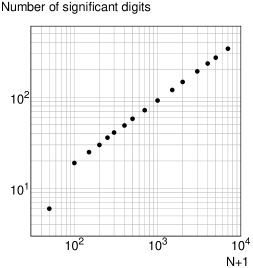
Figure 3: Number of significant digits of the ratio $\frac{f_{2}}{f_{0}}$, for ODE $(\ref{eqn:ex_2})$

Proportion $\rho$ defined in (47)

Figure 4: Proportion $\rho$ defined in $(\ref{eqn:def_ratio_digits})$, for ODE $(\ref{eqn:ex_2})$

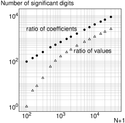
Figure 5: Number of significant digits of the ratio $\frac{f_{7}}{f_{5}}$ and Number of significant digits of the ratio $\frac{f(1/30)}{f(0)}$, for ODE $(\ref{eqn:ex_3})$

Proportion $\rho$ defined in (47)

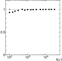
Figure 6: Proportion $\rho$ defined in $(\ref{eqn:def_ratio_digits})$, for ODE $(\ref{eqn:ex_3})$

Moreover, under the scale change $x\to 30x$, the accuracy is improved very much. Under this scale change, ODE (46) is modified to

$$\frac{1}{(30)^{2}}f^{\prime\prime}-(30)^{2}x^{2}f+(2\nu+1)f=0\,.$$ (48)

The results for this ODE with $\nu=0$, $k_{0}=6$, $K=2\lfloor\frac{7(N-k_{0})}{16}\rfloor+k_{0}$ and $J=2\lfloor\frac{15(N-k_{0})}{32}\rfloor+k_{0}$ are given in Fig 6. In this case, with $N\geq 100$, the number of the significant digits between two coefficients is infinite (i.e. perfectly exact ratio is obtained) when the true ratio is rational which occurs for the ratio among $f_{0},f_{1},\ldots,f_{5}$, and it is very large even when the true ratio is irrational. For example, for the ratio $\frac{f_{7}}{f_{5}}$ (which is irrational), the ratio obtained numerically by the proposed method coincides within 8783 digits to the true ratio when $N+1=30000$. Moreover, for the ratio between the values of the solution function at two points $\frac{f(1/30)}{f(0)}$, there the numerical result by the proposed method coincides within 2599 digits to the true ratio. (The number of significant digits seems to be proportional to $N^{0.79}$ empirically in the case when $N$ is sufficiently large.) As for the ratio defined in (47), the numerical results by the proposed method give almost a ‘full precision’ al so in this case, which is shown in Fig 6. There results show evidently how accurate the proposed method is.

Next, we give examples in Fuchsian class where $p_{M}(x)$ has zero points. Here, we show how numerical results converge to true solutions in such a case where the true solutions are written with the associate Legendre function. In this case, we are successful to extract only the true solutions defined only in $(-1,1)$ by the proposed method, where the obtained solutions is almost zero outside these intervals.

Figure 7: Numerical result of functions for the associate Legendre differential equation $(\ref{eqn:ex_4}$)

An example of such a case is for the associate Legendre differential equation

$$(1-x^{2})f^{\prime\prime}-2xf^{\prime}+\left(\nu(\nu+1)-\frac{\mu^{2}}{1-x^{2}}\right)f=0.$$ (49)

By means of the discussion in Subsection 3.5, we can treat this ODE by the proposed algorithm as the Fuchsian-type ODE

$$(1-x^{2})^{2}f^{\prime\prime}-2x(1-x^{2})f^{\prime}+\left(\nu(\nu+1)(1-x^{2})-\mu^{2}\right)f=0$$ (50)

whose coefficient functions are polynomials. As is well known, there are three intervals $(-\infty,-1)$, $(-1,1)$ and $(1,\infty)$ within which smooth solutions are defined, because the coefficient function $p_{2}(x)$ of the highest order term has two zero points $x=\pm 1$. However, none of the solutions defined in the intervals $(-\infty,-1)$ and $(1,\infty)$ is square-integrable, and hence the space of solutions in $L_{(k_{0})}^{2}(\mathbb{R})$ ($\subset L^{2}(\mathbb{R})$) is the one-dimensional space $\{C\cdot 1_{[-1,1]}(x)\cdot(1-x^{2})^{\frac{\mu}{2}}L_{\nu}^{\mu}(x)\,|\,C\in\mathbb{C}\}$   ($1_{I}(x)$: indicator function, $(1-x^{2})^{\frac{\mu}{2}}L_{\nu}^{\mu}(x)$: associate Legendre function). The results for this ODE with $\mu=3$, $\nu=4$, $k_{0}=6$, $K=2\lfloor\frac{7(N-k_{0})}{16}\rfloor+k_{0}$, $J=2\lfloor\frac{15(N-k_{0})}{32}\rfloor+k_{0}$ and $N+1=50,100$ are given in Fig 7. Note that there the solutions are normalized by $\,\langle f,\frac{1}{2\pi}(\psi_{k_{0},0}+\psi_{k_{0},-k_{0}-1})\rangle_{{\cal H}}=1$. Surprisingly, almost only the component in $\{C\cdot 1_{[-1,1]}(x)\cdot(1-x^{2})^{\frac{\mu}{2}}L_{\nu}^{\mu}(x)\,|\,C\in\mathbb{C}\}$ is ‘automatically’ extracted, and the numerical solutions are almost zero outside the interval $(-1,1)$, in spite of the existence of singularities at $x=\pm 1$. However, the convergence to the true solution is not so rapid as the cases where $p_{M}(x)$ has no zero points, though it converges to the true solution anyway.

For the ODEs whose exact solutions can be written by the (associate) Laguerre functions $x^{\frac{\mu}{2}}e^{-\frac{x}{2}}L_{\nu}^{\mu}(x)$ within the interval $(0,\infty)$, we have already had similar results to this, where the obtained numerical solutions are almost zero for $x<0$.

6 Discussion

6.1 Some properties of the basis functions used in this study

The basis systems $\{e_{n}\,\}_{n=0}^{\infty}$ and $\{e_{n}^{\Diamond}\}_{n=0}^{\infty}$ are closely related to Fourier series, by the change of variable $\theta=2\arctan x$, as is shown in subsection 2.4 of the paper  [8]. (The same change of variable has been used for a description of analytic unit quadrature signals with nonlinear phase [15] [16].)

The function $\psi_{k,\,0}$ is identical to the Cauchy wavelet [17] used for continuous wavelet transformation [18]. Moreover, when $k$ is even, $\psi_{k,\,{\ddot{n}}}$ is closely related to the number state associated with $\mathfrak{su}(1,1)$ in a representation of $\mathfrak{su}(1,1)$ which can be formulated by adding a third generator to the two generators of the $ax+b$ group [19].

6.2 Extension to inhomogeneous differential equations

The algorithm proposed in this paper is easily extended to linear inhomogeneous ordinary differential equations with inhomogeneous terms in ${{\cal H}^{\Diamond}}$. This extension only requires substitution of the right hand side $0$ of the simultaneous linear equations $\sum_{n}b_{m}^{n}f_{n}=0$ $(m\in Z^{+})$ by the $\widetilde{H}$-inner-products between the inhomogeneous term and the basis function $e_{m}^{\Diamond}$.

6.3 Modification of the method for the eigenvalue-eigenvector problem

We have already proved that the proposed method can be applied for eigenfunction problems of self-adjoint operators with given eigenvalues, under some conditions, which will be reported in another paper [20]. In order to apply the proposed method to the eigenvalue-eigenvector problem for a linear operator, we must have a method to obtain the eigenvalues, because the eigenvalue is regarded as a fixed parameter of the characteristic equation in the proposed method. In the case of discrete eigenvalues, if an eigenvalue is not exact, the function satisfying the characteristic equation does not belong to ${\cal H}$, and hence its corresponding vector is not square-summable.

However, when we truncate the algorithm within a finite number of dimensions, the square-summability is not distinguishable. The number sequence obtained by our method for an approximate eigenvalue decays within a finite number of dimensions as rapidly as the number sequence corresponding to the true eigenvector. As the approximation of the eigenvalue is better, it decays for more dimensions. From this fact, we can propose a method to find the eigenvalue by observing the location of the bottom of the valley of the ratio $\sigma_{K}^{(\Omega)}$. Here we give an example of such valleys in Figure 9. In this example, we are successful to separate two eigenvalues which are very contiguous by the ‘tunnel effect’, for a Schrödinger equation with quantum-double-well-type potential function.

Figure 8: Example of ‘valleys’ of the ratio between the two norms

Figure 9: Possibility of a more precise interpolation by means of an index almost linear to the deviation

Moreover, we have already invented another faster and more effective method for finding eigenvalues in a very high accuracy, based on a more analytical idea. This idea utilizes linear interpolations by means of some indices almost linear to the deviation of the eigenvalue (see Fig.9) which are calculated directly from numerical results.

6.4 Possibility of the extension to partial differential equations

A similar idea to the proposed method can be applied to linear partial differential equations. However, the number of linearly independent solutions of simultaneous linear equations is not fixed but increasing as $N$ increases for linear partial differential equations, while it is fixed at $p=j_{0}+\ell_{0}-1$ for linear ordinary differential equations. Therefore, we have to estimate how much memory and how many calculations would be required.

6.5 Possibility of the extension to weakly non-linear differential equations

This algorithm has the possibility of extension to nonlinear differential equations because of the following properties: ¿From the definition of $\psi_{k_{0},{\ddot{n}}}$,   the relation $\psi_{k_{0},{\ddot{n}}_{1}}(x)\cdot\psi_{k_{0},{\ddot{n}}_{2}}(x)=\psi_{2k_{0}+1,\,{\ddot{n}}_{1}+{\ddot{n}}_{2}}(x)$ holds. The combination of this fact and Lemma 3.2 results in the fact that the product $\psi_{k_{0},{\ddot{n}}_{1}}(x)\cdot\psi_{k_{0},{\ddot{n}}_{2}}(x)$ can be expressed as a linear combination of $\psi_{k_{0},\,{\ddot{n}}_{1}+{\ddot{n}}_{2}}(x),\psi_{k_{0},\,{\ddot{n}}_{1}+{\ddot{n}}_{2}+1}(x),\ldots,\psi_{k_{0},\,{\ddot{n}}_{1}+{\ddot{n}}_{2}+k_{0}+1}(x)$. Similarly, the product of more than three basis functions can be written as a linear combination of finite numbers of the same basis functions. If the nonlinearity is weak, we can apply the proposed method to the successive approximation method for nonlinear differential equations, because of this property. However, for the nonlinear case, it is more difficult to find a proof of convergence and an upper bound for errors, than it is for the linear case.

7 Conclusions

We have proposed an integer-type algorithm which can determine accurately a basis system for the space of solutions in ${\cal H}$ of the $M$-th order ODE $\displaystyle\Bigl{(}\sum_{m=0}^{M}p_{m}(x)\bigl{(}{\textstyle\frac{d}{dx}}\bigr{)}^{m}\Bigr{)}f(x)=0$ with polynomials or rational functions for the coefficient functions $p_{m}$ $(m=0,\ldots,M)$ under certain conditions. The basic structure of this algorithm has been shown in a more general framework and several conditions have been stated for the validity of this structure. Next, we have provided choices for the spaces and their basis systems satisfying these conditions, with detailed checks of these conditions. Thus, the validity of the proposed method has been proved.

Moreover, we have shown convergence of the results of this method to true solutions of the differential equations, under the conditions required for the structure of the algorithm. Numerical results have indicated that this method has high accuracy. We have provided examples to show how the results converge to true solutions as the dimension of the subspace increases.

This method will be extended or generalized for inhomogeneous equations, partial equations and weakly nonlinear equations in the near future, as has been mentioned in Section 6. Analyses of the accuracy and the amount of calculations required are also future problems. Moreover, it is our intent to apply this method, with some modifications, to the scattering problem in quantum mechanics.

Appendix A Proof of Lemma 3.1

Proof of Lemma 3.1:  ¿From the last property of (29), $\{\sqrt{\frac{1}{\pi}}\,\psi_{k,\,{\ddot{n}}}\,|\,{\ddot{n}}\in\mathbb{Z}\}$ is orthonormal. Therefore, we have only to prove the completeness in $L_{(k)}^{2}(\mathbb{R})$. Let ${\cal F}$ be the Fourier transformation, where the Fourier transform of a function $f$ is denoted by $\displaystyle\bigl{(}{\cal F}f\bigr{)}(y):=\frac{1}{\sqrt{2\pi}}\int_{-\infty}^{\infty}f(x)e^{-iyx}\,dx$. Some calculations by residue calculus result in

$${}^{\forall}\ddot{n}\geq 0,\,\,\,\ ({\cal F}\psi_{0,\,{\ddot{n}}})(y)=\left\{\begin{array}[]{@{\,}ll}\displaystyle i\,\sqrt{2\pi}\,\,\,e^{-y}\,L_{\ddot{n}}(2y)&(y\geq 0)\\ \\ \displaystyle 0&(y<0)\end{array}\right.$$ (54)

where $L_{n}(x)$ denotes the Laguerre polynomial of degree $n$. On the other hand, since $\overline{\psi_{0,\,{\ddot{n}}}(x)}=\psi_{0,\,-{\ddot{n}}-1}(x)$ from (29), a property of the Fourier transform leads us to

$${}^{\forall}\ddot{n}\geq 0,\,\,\,\ ({\cal F}\psi_{0,\,-{\ddot{n}}-1})(y)=\left\{\begin{array}[]{@{\,}ll}\displaystyle-i\,\sqrt{2\pi}\,\,\,e^{\,y}\,L_{\ddot{n}}(-2y)&(y\leq 0)\\ \\ \displaystyle 0&(y>0).\end{array}\right.$$ (58)

Here, let

$${\cal L}_{(0)}^{-} := \bigl{\{}\,\sum_{{\ddot{n}}=-\infty}^{-1}\xi_{\ddot{n}}\,\psi_{0,\,{\ddot{n}}}(x)\,\,\bigl{|}\,\,\xi_{\ddot{n}}\in{\mathbb{C}},\,\,\{\xi_{\ddot{n}}\}\in\ell^{2}(\mathbb{Z}\backslash\mathbb{Z}^{+})\,\bigr{\}},$$

$${\cal L}_{(0)}^{+} := \bigl{\{}\,\sum_{{\ddot{n}}=0}^{\infty}\xi_{\ddot{n}}\,\psi_{0,\,{\ddot{n}}}(x)\,\,\bigl{|}\,\,\xi_{\ddot{n}}\in{\mathbb{C}},\,\,\{\xi_{\ddot{n}}\}\in\ell^{2}(\mathbb{Z}^{+})\,\bigr{\}}\,\,.$$

Then, from the well-known fact that the set $\{\,e^{-\frac{t}{2}}\,L_{n}(t),\,\,t\geq 0\,\,|\,\,n\in\mathbb{Z}^{+}\}$ is complete in $L^{2}\bigr{(}\,\mathbb{R}^{+}\,\bigr{)}\,,$ we can show that $\{\,{\cal F}f\,\,|\,f\in{\cal L}_{(0)}^{+}\}=L^{2}\bigr{(}\,\mathbb{R}^{+}\,\bigr{)}$. Similarly, from (58) and this fact, $\{\,{\cal F}f\,\,|\,f\in{\cal L}_{(0)}^{-}\}=L^{2}\bigr{(}\,\mathbb{R}^{-}\,\bigr{)}$. Since the null functions in $L^{2}(\mathbb{R})$ which are nonzero only at $y=0$ in the frequency domain belong to the kernel of the inverse Fourier transformation, from the Planchrel theorem,

$$L^{2}(\mathbb{R})={\cal L}_{0}^{-}\oplus{\cal L}_{0}^{+}\,=\,\bigl{\{}\,\sum_{{\ddot{n}}=-\infty}^{\infty}\xi_{\ddot{n}}\,\psi_{0,\,{\ddot{n}}}(x)\,\,\bigl{|}\,\,\xi_{\ddot{n}}\in{\mathbb{C}},\,\,\{\xi_{\ddot{n}}\}\in\ell^{2}(\mathbb{Z})\,\bigr{\}}\,\,,$$ (59)

and hence $\{\sqrt{\frac{1}{\pi}}\,\psi_{0,{\ddot{n}}}\,|\,{\ddot{n}}\in\mathbb{Z}\}$ is complete in $L^{2}(\mathbb{R})=L_{(0)}^{2}(\mathbb{R})$. Then, since $\displaystyle\,\psi_{k,\,{\ddot{n}}}(x)=\frac{\psi_{0,\,{\ddot{n}}}(x)}{(x+i)^{k}}\,$, from (25) and (59),

$$L_{(k)}^{2}(\mathbb{R}) = \bigl{\{}\,\frac{1}{(x+i)^{k}}\sum_{n=-\infty}^{\infty}\xi_{n}\,\psi_{0,\,{\ddot{n}}}(x)\,\,\bigl{|}\,\,\xi_{\ddot{n}}\in{\mathbb{C}},\,\,\{\xi_{\ddot{n}}\}\in\ell^{2}(\mathbb{Z})\,\bigr{\}}$$

$$= \bigl{\{}\,\sum_{{\ddot{n}}=-\infty}^{\infty}\xi_{\ddot{n}}\,\psi_{k,\,{\ddot{n}}}(x)\,\,\bigl{|}\,\,\xi_{\ddot{n}}\in{\mathbb{C}},\,\,\{\xi_{\ddot{n}}\}\in\ell^{2}(\mathbb{Z})\,\bigr{\}}\,\,,$$

and hence $\{\sqrt{\frac{1}{\pi}}\,\psi_{k,{\ddot{n}}}\,|\,{\ddot{n}}\in\mathbb{Z}\}$ is complete in $L_{(k)}^{2}(\mathbb{R})$.   

Appendix B Proof of Theorem 3.2

For the proof of Theorem 3.2, here we start with the following lemma which is based on the translation of Lemma 3.2 by the ‘matching’ used in (33):

Lemma B.1

Let $k_{0},j,m\in\mathbb{Z}^{+}$, $\kappa\in\mathbb{Z}$ and $\,\ell_{1}:=2m+k_{0}-\kappa$. Under the choices (26), (27), and (33), for $\,\kappa\leq k_{0}+m-j$, the function $x^{j}({\textstyle\frac{d}{dx}})^{m}e_{n}(x)$ can be expressed as a linear combination of $e_{n^{\prime}}^{\Diamond}$ $(n^{\prime}=0,1,...n+\ell_{1})$ at most for $n<\ell_{1}$, and it can be expressed as a linear combination of $e_{n^{\prime}}^{\Diamond}$ $(n^{\prime}=n-\ell_{1},\,n-\ell_{1}+2,\,n-\ell_{1}+4,\,n-\ell_{1}+6,\,....,n+\ell_{1})$ for $n\geq\ell_{1}$. In these linear combinations, all the coefficients are polynomials of ${\ddot{n}}_{k_{0},n}$ and $k_{0}$ with degree not greater than $m$. In particular, in the linear combination for $n\geq\ell_{1}$, with ${\ddot{n}}_{k_{0},n}$ defined in (33), the coefficient of the first term with $e_{n-\ell_{1}}^{\Diamond}$ is $\,\displaystyle\left(\frac{i}{2}\right)^{k_{0}-\kappa-j+m}\left(\frac{1}{2}\right)^{j}(-1)^{m}\prod_{t=1}^{m}\left({\ddot{n}}_{k_{0},n}+k_{0}+t\right)$ when $n+k_{0}$ is even, and it is $\,\displaystyle\left(-\frac{i}{2}\right)^{k_{0}-\kappa-j+m}\left(\frac{1}{2}\right)^{j}\prod_{t=1}^{m}\left({\ddot{n}}_{k_{0},n}-t+1\right)$ when $n+k_{0}$ is odd.

The proof is derived directly from Lemma 3.2 together with (33).

Proof of Theorem 3.2:  From the definition of $s_{0}$, the inequality ${k_{0}^{\Diamond}}\leq k_{0}-s_{0}$ implies that ${}^{\forall}m\in\{0,1,2,...,M\},\,\,\,{k_{0}^{\Diamond}}\leq k_{0}+m-\deg p_{m}$. Hence for every term in the expansion $\displaystyle P(x,{\textstyle\frac{d}{dx}})=\sum_{m=0}^{M}\sum_{j=0}^{\deg p_{m}}p_{m.j}\,x^{j}({\textstyle\frac{d}{dx}})^{m}$, ${k_{0}^{\Diamond}}\leq k_{0}+m-j$ holds. Therefore, we can apply Lemma B.1 term-wise in this expansion, where $\langle x^{j}({\textstyle\frac{d}{dx}})^{m}e_{r},e_{n}^{\Diamond}\rangle_{{{\cal H}^{\Diamond}}}=0$ for

$|r-n|>2m+k_{0}-{k_{0}^{\Diamond}}$ and of course for $|r-n|>2M+k_{0}-{k_{0}^{\Diamond}}$. Hence

$b_{n}^{r}=\langle Be_{r},\,e_{n}^{\Diamond}\rangle_{{{\cal H}^{\Diamond}}}=0$ for $|r-n|>2M+k_{0}-{k_{0}^{\Diamond}}$  1.e. (a) holds.

Next, we will show (b). Since ${\ddot{n}}_{k_{0},r}:=\lfloor-{\textstyle\frac{k_{0}+1}{2}}\rfloor+(-1)^{r+k_{0}+1}\,\lfloor{\textstyle\frac{r+1}{2}}\rfloor$,

$\displaystyle|{\ddot{n}}_{k_{0},r}|\leq\frac{r+k_{0}+4}{2}$. Hence, for fixed $k_{0}$, for any polynomial $B(x)$, there exists a polynomial $A(x)$ of the same degree as $B(x)$ such that $|B({\ddot{n}}_{k_{0},r})|\leq A_{m}(r)$ for $r\in\mathbb{Z}^{+}$. Since Lemma B.1 implies that there exists a polynomial $B_{(n)}(x)$ of degree not greater than $M$ such that $b_{n}^{r}=B_{(n)}(r)$ for every $n\in\mathbb{Z}^{+}$, this fact results in the existence of a polynomial $A(x)$ of degree not greater than $M$ such that $|b_{n}^{r}|\leq A(r)$ for $r\in\mathbb{Z}^{+}$,  i.e. (b) holds.

Moreover, for $m<M-1$, $\displaystyle\left\langle x^{j}{\textstyle(\frac{d}{dx})}^{m}e_{r},\,e_{r-(2M+k_{0}-{k_{0}^{\Diamond}})}^{\Diamond}\right\rangle_{{{\cal H}^{\Diamond}}}=0$ because

$|r-(r-(2M+k_{0}-{k_{0}^{\Diamond}}))|>2m+k_{0}-{k_{0}^{\Diamond}}$. Hence

$\displaystyle b_{r+2M+k_{0}-{k_{0}^{\Diamond}}}^{r}=\langle Be_{r},e_{r+2M+k_{0}-{k_{0}^{\Diamond}}}^{\Diamond}\rangle_{{{\cal H}^{\Diamond}}}=\left\langle p_{M}(x){\textstyle(\frac{d}{dx})}^{M}e_{r},e_{r-(2M+k_{0}-{k_{0}^{\Diamond}})}^{\Diamond}\right\rangle_{{{\cal H}^{\Diamond}}}$. On the other hand, with ${\ddot{n}}_{k_{0},r}:=\lfloor-{\textstyle\frac{k_{0}+1}{2}}\rfloor+(-1)^{r+k_{0}+1}\,\lfloor{\textstyle\frac{r+1}{2}}\rfloor$, Lemma B.1 implies that

$$\left\langle x^{j}{\textstyle(\frac{d}{dx})}^{M}e_{r},\,e_{r-(2M+k_{0}-{k_{0}^{\Diamond}})}^{\Diamond}\right\rangle_{{{\cal H}^{\Diamond}}}$$

$$=\left\{\begin{array}[]{@{\,}ll}\displaystyle(-i)^{j}\,\left(\frac{i}{2}\right)^{k_{0}-{k_{0}^{\Diamond}}+M}(-1)^{M}\prod_{t=1}^{M}\left({\ddot{n}}_{k_{0},r}+k_{0}+t\right)&\,\,\,\,\,({\rm if}\,\,\,k_{0}+r:{\rm even})\\ \\ \displaystyle i^{j}\,\left(-\frac{i}{2}\right)^{k_{0}-{k_{0}^{\Diamond}}+M}\prod_{t=1}^{M}\left({\ddot{n}}_{k_{0},r}-t+1\right)&\,\,\,\,\,({\rm if}\,\,\,k_{0}+r:{\rm odd})\end{array}\right.$$

holds for $r\geq 2M+k_{0}-{k_{0}^{\Diamond}}$, because $\displaystyle\left(\frac{1}{2}\right)^{j}=(\mp i)^{j}\left(\frac{\pm i}{2}\right)^{j}$. These facts and the relation $\displaystyle\sum_{j=0}^{\deg p_{M}}p_{M,j}\,(\pm i)^{j}=p_{M}(\pm j)$ for $r\geq 2M+k_{0}-{k_{0}^{\Diamond}}$ imply that

$$\left\langle Be_{r},\,e_{r-(2M+k_{0}-{k_{0}^{\Diamond}})}^{\Diamond}\right\rangle_{{{\cal H}^{\Diamond}}}$$

$$=\left\{\begin{array}[]{@{\,}ll}\displaystyle p_{M}(-i)\,\,\left(\frac{i}{2}\right)^{k_{0}-{k_{0}^{\Diamond}}+M}(-1)^{M}\prod_{t=1}^{M}\left({\ddot{n}}_{k_{0},r}+k_{0}+t\right)&\,\,\,\,\,({\rm if}\,\,\,k_{0}+r:{\rm even})\\ \\ \displaystyle p_{M}(i)\,\,\left(-\frac{i}{2}\right)^{k_{0}-{k_{0}^{\Diamond}}+M}\prod_{t=1}^{M}\left({\ddot{n}}_{k_{0},r}-t+1\right)&\,\,\,\,\,({\rm if}\,\,\,k_{0}+r:{\rm odd}).\end{array}\right.$$

¿From the definition of ${\ddot{n}}_{k_{0},r}$, at least with $r\geq k_{0}+2M$,  ${\ddot{n}}_{k_{0},r}+k_{0}+t\leq-2$ for

$t=0,1,2,...,M$ when $k_{0}+r$ is even and ${\ddot{n}}_{k_{0},r}-t+1\geq 1$ for $t=0,1,2,...,M$ when $k_{0}+r$ is odd (where $r=k_{0}+2M$ is impossible). Since $p_{M}(\pm i)\neq 0$ from the condition, we have the conclusion $\left\langle Be_{r},\,e_{r-(2M+k_{0}-{k_{0}^{\Diamond}})}^{\Diamond}\right\rangle_{{{\cal H}^{\Diamond}}}\neq 0$ at least for

$r\geq k_{0}+2M+\max(-{k_{0}^{\Diamond}},\,0)$ i.e. (c) holds.

References

- [1] E. A. Coddington and N. Levinson, Theory of Ordinary Differential Equations, McGraw-Hill, New York (1955).
- [2] A. W. Eldély et al., Higher transcendental functions, 3 vols., McGraw-Hill, New York (1953-55).
- [3] A. Messiah, Quantum mechanics, Dover, New York (1999).
- [4] M. A. Krasnosel’slii, G. M. Vainikko, P. P. Zabreiko, Y. B. Rutitskii, and V/Y. Stetsenko, Approximate Solution of Operator Equations, translated by D. Louvish, Wolters-Noordhoff Publishinf, Groningen (1972).
- [5] S. C. Brenner and L. R. Scott, The Mathematical Theory of Finite Element Methods, 2nd. ed., Springer, New York (2007).
- [6] A. Ern and J. L. Guermond, Theory and Practice of Finite Elements, Springer, New York (2004).
- [7] F. Sakaguchi and M. Hayashi, Practical implimentation and error bound of integer-type algorithm for higher order differential equations, arXive:0903.4850.
- [8] F. Sakaguchi and M. Hayashi, Differentiability of eigenfunctions of the closures of differential operators with rational coefficient functions, arXive:0903.4852.
- [9] D. Gilbarg and N. S. Trudinger, Elliptic Partial Differential Equations of Second Order Springer-Verlag, Berlin 1998.
- [10] M. Reed and B. Simon, Methods of Modern Mathematical Physics I: Functional analysis, Academic Press, New York (1980).
- [11] Mathematical Society of Japan, Encyclopedic Dictionary of Mathematics, 2nd ed., Vol.II, ed. by K. Itô, items 254.A and 254.B, The MIT Press, Cambridge (1987).
- [12] E. Hille, Ordinary Differential Equations in the Complex Domain, John Wiley and Sons, New York (1976).
- [13] A. K. Lenstra, H. W. Lenstra Jr, and L. Lovász, Factoring polynomials with rational coefficients, Math. Ann. 261, 515-534 (1982).
- [14] L. Babai, On Lovász’ lattice reduction and the nearest lattice point problem, Combinatorica, 6(1), 1-13 (1986).
- [15] T. Qian et al., Analytic unit quadrature signals with nonlinear phase, Physica D, 203, 80-87 (2005).
- [16] Q. Chen et el., Two families of unit analytic signals with nonlinear phase, Physica D, 221, 1-12 (2006).
- [17] M. Holschneider, Wavelets: an Analysis Tool. Oxford, Clarendon Press (1995).
- [18] I. Daubechies, Ten Lectures on Wavelets, SIAM, Philadelphia (1992).
- [19] F. Sakaguchi and M. Hayashi, Coherent states and annihilation-creation operators associated with the irreducible unitary representations of , J. Math. Phys., 43, 2241-2248 (2002).
- [20] F. Sakaguchi and M. Hayashi, Integer-type algorithm for eigenfunction/eigenvalue problem of self-adjoint operators and its application to Schrödinger operators (in preparation).