Fictitious Play in $3\times 3$ Games: chaos and dithering behaviour

Abstract

In the 60’s Shapley provided an example of a two player fictitious game with periodic behaviour. In this game, player $A$ aims to copy $B$’s behaviour and player $B$ aims to play one ahead of player $A$. In this paper we continue to study a family of games which generalize Shapley’s example by introducing an external parameter, and prove that there exists an abundance of periodic and chaotic behavior with players dithering between different strategies. The reason for all this, is that there exists a periodic orbit (consisting of playing mixed strategies) which is of ‘jitter type’: such an orbit is neither attracting, repelling or of saddle type as nearby orbits jitter closer and further away from it in a manner which is reminiscent of a random walk motion. We prove that this behaviour holds for an open set of games.

1 Introduction

The purpose of this paper is to show how complicated the dynamics of fictitious play can be (for an interpretation of fictitious play as a model for rational learning, see for example Fudenberg and Levine [1998]). We do this by analysing in detail the following family of $3\times 3$ games determined by the matrices

$$A_{\beta}=\left(\begin{array}[]{ccc}1&0&\beta\\ \beta&1&0\\ 0&\beta&1\end{array}\right)\quad B_{\beta}=\left(\begin{array}[]{ccc}-\beta&1&0\\ 0&-\beta&1\\ 1&0&-\beta\end{array}\right),$$ (1.1)

which depend on a parameter $\beta\in(0,1)$ (and best response dynamics given by the differential inclusion (1.2)). In fact, we shall show in Theorem 1.4 that our results even hold for matrices $A,B$ with

$$||A-A_{\beta}||,||B-B_{\beta}||\leq\epsilon\mbox{ with }\epsilon>0\mbox{ small}.$$

However, except for Theorem 1.4 and Section 6, we shall simply write $A=A_{\beta}$ and $B=B_{\beta}$. As usual, player $A$ has utility $p^{A}Ap^{B}$ whereas player $B$ has utility $p^{A}Bp^{B}$ where the row vector $p^{A}\in\Sigma_{A}\subset{\mathbb{R}}^{3}$ denoted the position of player $A$ and the column vector $p^{B}\in\Sigma_{B}\subset{\mathbb{R}}^{3}$ the position of player $B$. For later use we write $v^{A}=Ap^{B}$ and $v^{B}=p^{A}B$. Here $\Sigma_{A},\Sigma_{B}$ are the set of probability vectors in ${\mathbb{R}}^{3}$. In other words, $\Sigma:=\Sigma_{A}\times\Sigma_{B}$ is the product of two-dimensional triangles and so topologically it is a ball in ${\mathbb{R}}^{4}$. Player $B$ (resp. $A$) is indifferent between all three strategies when $p^{A}=E^{A}$, $p^{B}=E^{B}$ and $E=(E^{A},E^{B})$ is the Nash equilibrium of the game. For the game $A=A_{\beta}$, $B=B_{\beta}$ one has $E^{A}:=(1/3,1/3,1/3)$ and $E^{B}:=(1/3,1/3,1/3)^{\prime}$.

For $\beta=0$ the game $A,B$ is equivalent to the classical example introduced by Shapley [1964] (where each of the players eventually chooses strategies periodically). For $\beta=(\sqrt{5}-1)/2\approx 0.618$, the game is equivalent to a zero-sume game (rescaling $B$ to $\tilde{B}=\sigma(B-1)$ gives $A+\tilde{B}=0$), so then [1951] play always converges to the interior equilibrium $E^{A},E^{B}$.

The best response $BR_{A}(p^{B})$ of player $A$ is the $i$-th unit vector if the $i$-th component of $v^{A}$ is larger than the other components of $v^{A}$ (if several components of $v^{A}$ are equally large, then $BR_{A}(p^{B})$ is the convex combination of unit vectors corresponding to the largest components of $v^{A}$). Define $BR_{B}(p^{A})$ similarly. Once best responses are selected, the dynamics is determined by moving in a straight line towards the best responses. In some of the literature this is done by taking the piecewise linear differential equation

$$\begin{array}[]{ll}{dp^{A}}/{dt}&=BR_{A}(p^{B})-p^{A}\\ {dp^{B}}/{dt}&=BR_{B}(p^{A})-p^{B}\end{array}$$ (1.2)

whereas others take

$$\begin{array}[]{ll}{dp^{A}}/{ds}&=\,\,(1/s)\,(BR_{A}(p^{B})-p^{A})\\ {dp^{B}}/{ds}&=\,\,(1/s)\,(BR_{B}(p^{A})-p^{B}).\end{array}$$ (1.3)

The orbits are the same in both cases, only the time parametrisation of the orbits differs (take $s=e^{t}$); for the latter, orbits slow down and a periodic orbit of period $T$ (1.2) corresponds to an orbit of (1.3) which returns in time $e^{T},e^{2T},e^{3T},\dots$. Equations (1.2) and (1.3) determine the dynamics up until such time as one or other (or both) players become indifferent between two (or more) pure strategies. When one or more of the players is indifferent between two strategies their dynamics may not be uniquely determined. So (1.2) and (1.3) are in fact differential inclusions rather than differential equations, but as the best response correspondences $p^{B}\mapsto BR_{A}(p^{B})$ and $p^{A}\mapsto BR_{B}(p^{A})$ are upper semicontinous with values closed, convex sets, it follows from Aubin and Cellina [1984, Chapter 2.1] that through each initial value there exists at least one solution which is Lipschitz continuous and defined for all positive time. It is shown in Hofbauer [1995] that, under mild regularity conditions (which are satisfied in our case), any solution is piecewise linear.

In fact, when the matrices (1.1) are chosen, play is not affected at all by this ambiguity except at $E$ (because a certain transversality condition is satisfied, see Sparrow [2008]). In other words, all the orbits (except the one through $E$) are uniquely determined (outside $E$, the dynamics is not affected by a choice of tie-breaking rule). Moreover, when $\beta\in(0,1)$ the flow is continuous except at $E$ (when $\beta\neq\sigma$, for a proof, see Sparrow et al [2008]).

Note that the best response of $A$ to any $p^{B}\neq E^{B}$ is either an integer $i\in\{1,2,3\}$ or a mixed strategy set $\bar{i}$ where $\bar{i}:=\{1,2,3\}\setminus\{i\}$ corresponding to where player $A$ is indifferent between two strategies but will not play $i$. Similarly for $B$. Hence one can associate to any orbit $(p^{A}(t),p^{B}(t)$ outside $E$, a sequence of times $t_{0}:=0<t_{1}<t_{2}<\dots$ and a sequence of best-response strategies $(i_{0},j_{0}),(i_{1},j_{i}),(i_{2},j_{2}),\dots$ where

$$(i_{n},j_{n})=(BR^{A}(p^{B}(t),BR^{B}(p^{A}(t))\mbox{ for }t\in(t_{n},t_{n+1})$$

with $i_{n}$ and $j_{n}$ equal to $1$, $2$, $3$, $\bar{1}$, $\bar{2}$ or $\bar{3}$ for each $n=0,1,2,\dots$. In Sparrow et al [2008] we showed that there are three periodic orbits: one for $\beta\in(0,\sigma)$ with play $(1,2),(2,2)$, $(2,3)$, $(3,3)$, $(3,1)$, $(1,1)$ (the Shapley orbit), one for $\beta\in(\sigma,1)$ with cyclic play $(1,3),(1,2),(3,2),(3,1)$, $(2,1),(2,3)$ and a third one with a period 6 orbit of mixed strategies $(\bar{1},\bar{1}),(\bar{1},\bar{2}),(\bar{2},\bar{2}),(\bar{2},\bar{3}),(\bar{3},\bar{3}),(\bar{3},\bar{1})$. The latter sequence of strategies correspond to a fully-invariant set $C(\Gamma)$ (so an orbit starting in this set remains in this set, and an orbit starting outside this set remains outside this set); this fully invariant set exists for each $\beta\in(0,1)$ and contains a periodic orbit when $\beta\in(\sigma,1)$. The latter orbit is of ‘jitter type’: it is neither attracting, repelling or of saddle type; instead nearby orbits jitter closer and further away from it in a manner which is reminiscent of a random walk motion. We describe this behavior in the final sections of this paper.

1.1 Abundance of Periodic Play

Let us state now the main results of this paper. To do this, let us say that an orbit of the game has cyclic play of period $n$ if the associated sequence $(i_{n},j_{n})$ is periodic: $(i_{k+n},j_{k+n})=(i_{k},i_{k})$ for all $k=0,1,\dots$. Given $k\in\{0,\dots,n-1\}$ we say that the players are indecisive at the $k$-th step if $k\geq 3$ and moreover

$$\{i_{k-3},i_{k-2},j_{k-1},i_{k}\}\neq\{1,2,3\}\mbox{ {\bf and } }\{j_{k-3},j_{k-2},j_{k-1},j_{k}\}\neq\{1,2,3\}$$

holds (so during this and the previous three moves, both players never deviated from a choice of two strategies). Sometimes we also will say that the players dither at the $k$-step. In the opposite case, we say the $k$-th step is decisive. The essential period of a cyclic play of period $n$ is the number of decisive steps $k\leq n$. For example, the cycle of period $6$

$$(1,2),(2,2),(2,3),(3,3),(3,1),(1,1)$$

never dithers whereas for the cycle of period $7$

$$(1,2),(2,2),(2,3),(3,3),(3,2),(3,1),(1,1)$$

players dither in the 5th step, so the essential period is again 6. Let $\sigma=(\sqrt{5}-1)/2\approx 0.618$.

Theorem 1.1.

[An abundance of periodic play] For each $\beta\in(0,1)$ and each $n\geq 1$ there are infinitely many different orbits $\gamma_{s}$, $s=1,2,\dots$ of the differential equation (1.2) (and of (1.3)) with corresponding cyclic play of period $N_{s}\to\infty$ as $s\to\infty$ but with essential period equal to $6n$. Moreover,

• for $\beta\in(0,\sigma)$, these orbits with cyclic play reach the interior equilibrium $E$ in finite time;

• for $\beta\in(\sigma,1)$ these orbits with cyclic play are genuine periodic orbits of (1.2) (and of (1.3)).

In Sparrow et al [2008] we showed that for $\beta\in(-1,\sigma)$ there exists a periodic orbit corresponding to cyclic play $(1,2),(2,2),(2,3),(3,3),(3,1),(1,1)$ (the Shapley orbit) which attracts an open set of initial conditions; the above theorem shows that many periodic orbits are not attracted to this cycle. In that paper it was also shown that for $\beta\in(\sigma,1)$ there exists another periodic orbit corresponding to cyclic play $(1,3),(1,2),(3,2),(3,1),(2,1),(2,3)$ (the anti-Shapley orbit) which becomes attracting when $\sigma\in(\tau,1)$ where $\tau\approx 0.915$. Again this attracting orbit does not attract everything.

That the players can have infinitely many orbits with the same essential period, is a consequence of the fact that there is a sequence of periodic orbits converging to the orbit of mixed strategies $(\bar{1},\bar{1}),(\bar{1},\bar{2}),(\bar{2},\bar{2}),(\bar{2},\bar{3}),(\bar{3},\bar{3}),(\bar{3},\bar{1})$, and which all have the same essential period. For these periodic orbits, the essential period is the number of times it follows the period 6 orbit before returning to its original position, whereas the actual period increases if the players dither for longer along each of the 6 legs. Along these periodic orbits at any given moment only one of the players is indifferent, but they dither for a long time between each decisive move.

Let us relate this theorem to a result of Krishna and Sjöström [1998] (which builds on earlier work of Rosenmüller [1971]). In this interesting paper, they show that for a generic game (i.e. for Lebesgue almost all pay-off matrices) there exists no open set of initial conditions for which fictitious play converges cyclically to a mixed strategy equilibrium (unless both players use at most two pure strategies). In other words, if fictitious play converges to a mixed strategy equilibrium with both players using more than two strategies then the choice of strategies cannot follow a cyclic pattern unless possibly the initial conditions are in some codimension-one space. Our result shows that for $\beta\in(0,\sigma)$ countably many orbits do indeed converge cyclically to the equilibrium (and along these orbits at any given moment only one of the players is indifferent). Our result does not rely on the symmetry of the matrices: it holds for an open set of matrices, see Theorem 1.4 and Section 6.

For their result, Krishna and Sjöström only only needed to consider orbits for which at any given moment only one of the players is indifferent. It is interesting to note however that, as becomes clear from this paper, it is precisely near the set $C(\Gamma)$ where both players are simultaneously indifferent that much of the interesting behaviour happens (and this set ’organises’ the local dynamics).

1.2 Abundance of Dithering Behavior

The next theorem shows that there are many orbits which dither for very long periods. To make this precise, let us assume the players start at $p\in\Sigma$ and aim for $(i_{0},j_{0}),(i_{1},j_{1}),(i_{2},j_{2}),\dots$. Next associate to these moves a sequence $(R_{k})_{k\geq 3}$ with $R_{k}\in\{D,I\}$, where $R_{k}$ is equal to $D$ or $I$ depending on whether the players are decisive or indecisive at time $k\geq 3$. In this way we get a map

$$\Sigma\ni p\mapsto\{R_{k}(p)\}_{k\geq 3}\in\{D,I\}^{\mathbb{N}}$$

which captures partly what play evolves from starting position $p\in\Sigma$. (We ignore $k<3$ because by definition the players are then always decisive. More precisely, if $T$ denotes the map which assigns to $(i_{k},j_{k})_{k\geq 0}$ the sequence $(R_{k})_{k\geq k_{0}}$ and $\sigma$ the shift map, then $T\circ\sigma=\sigma\circ T$ only if we take $k_{0}\geq 3$.)

To simplify the coding even further, define the times $3\leq N_{0}(p)<N_{1}(p)<N_{2}(p)<\dots$ for which the players are decisive (only considering times $\geq 3$). Note that these times uniquely determine again the sequence $R_{3}(p),R_{4}(p),\dots$  . If $N_{s+1}(p)-N_{s}(p)$ is large, then we say that the players dither for a long time (as they then each play back and forth between two strategies).

Theorem 1.2.

[There is a lot of freedom in the choice of dithering sequences] For each $\beta\in(0,1)$ there exist $N^{0}\in{\mathbb{N}}$, $0<\lambda<1<\mu$ and a compact set $X\subset\Sigma$, so that for each sequence $N_{0}<N_{2}<N_{4}<\dots$ with $N_{0}\geq 3$ and with

$$\lambda\leq\frac{N_{2s+4}-N_{2s+2}}{N_{2s+2}-N_{2s}}\leq\mu\mbox{ and }N_{2s+2}-N_{2s}\geq N^{0}\mbox{ for all }s\geq 0$$

there exists $p\in X$ such that

$$|N_{2s}(p)-N_{2s}|\leq 4\mbox{ for all }s\geq 0.$$

Moreover,

• for $\beta\in(0,\sigma)$ orbits in $X$ converge to $E$;

• for $\beta\in(\sigma,1)$ orbits starting in $X$ do not converge to $E$.

That this theorem only refers to the gaps between even decisive moments, $N_{2s+2}-N_{2s}$, is because the gaps between the even and odd moments are somewhat more arbitrary. However, if $N_{2s+2}(p)-N_{2s}(p)$ is large for all $s\geq 0$, then $N_{s+1}(p)-N_{s}(p)$ is also large for all $s\geq 0$, i.e., the players dither for long periods between making a decisive move for orbits described above.

We did some numerical simulations for games determined by completely different matrices. In many of these, similar dithering behaviour also occurred. Even for zero-sum games, the players seem to converge to equilibria in a dithering fashion (in fact, in $2\times n$ games, dithering is unavoidable). We will report on these simulations in a subsequent paper.

1.3 Chaotic Behavior

The previous theorem states that there are orbits starting in $X$ which dither for more or less arbitrary lengths $N_{2s+2}-N_{s}$. An immediate application of this theorem is the following result:

Theorem 1.3 (Chaos).

Take $\hat{N}\geq N^{0}$ so large that $\lambda\leq(\hat{N}-1)/\hat{N}\leq(\hat{N}+1)/\hat{N}\leq\mu$. For each sequence $(\epsilon_{2s})_{s\geq 0}$ with $\epsilon_{2s}\in\{-5,0,5\}$ there exists $p\in X$ with

$$N_{2s+2}-N_{2s}\in[\hat{N}+\epsilon_{2s},\hat{N}+4+\epsilon_{2s}]\mbox{ for all }s\geq 0.$$

So for such a $p$,    $N_{2s+2}-N_{2s}$ is in the interval $[\hat{N}-5,\hat{N}-1]$, $[\hat{N},\hat{N}+4]$ or $[\hat{N}+5,\hat{N}+9]$ depending on the parity of $\epsilon_{2s}$. In particular the flow contains subshifts of finite type and has positive topological entropy. The flow also has sensitive dependence on initial conditions.

The definition of the notions ‘subshifts of finite type’, ‘positive topological entropy’ and ‘sensitive dependence on initial conditions’ can be found in almost any book on dynamical systems, for example Guckenheimer and Holmes [1983]. We have numerical evidence that this game is chaotic in a more profound sense: it appears that there exists a range of parameters $\beta\in(\sigma,\tau)$ so that (Lebesgue) almost all starting positions correspond to chaotic behaviour. We will report on this in a subsequent paper.

1.4 Robustness

The above results do not require the matrices to be of a special form, and hold for games corresponding to an open set of matrices:

Theorem 1.4 (Robustness).

For each $\beta\in(0,1)$ with $\beta\neq\sigma$, there exists $\epsilon>0$ so that for each $3\times 3$ matrices $A$ and $B$ with

$$||A-A_{\beta}||,||B-B_{\beta}||<\epsilon$$

the previous theorems also hold. More precisely,

• for $\beta\in(0,\sigma)$ and $\epsilon>0$ sufficiently small,

  • there exists a periodic orbit corresponding to cyclic play $(1,2)$, $(2,2)$, $(2,3)$, $(3,3)$, $(3,1)$, $(1,1)$ (the Shapley orbit) which attracts an open set of initial conditions;

  • there exist orbits of mixed strategies $(\bar{1},\bar{1}),(\bar{1},\bar{2}),(\bar{2},\bar{2}),(\bar{2},\bar{3}),(\bar{3},\bar{3}),(\bar{3},\bar{1})$; such orbits lie on a cone with apex $E$; all orbits on this cone converge to $E$; there are infinitely many different orbits $\gamma_{s}$, $s=1,2,\dots$ as in Theorem 1.1 which reach the interior equilibrium $E$ in finite time;

  • there are orbits which dither as in Theorem 1.2 which again reach the interior equilibrium $E$ in finite time;

• for $\beta\in(\sigma,1)$ and $\epsilon>0$ sufficiently small,

  • there exist a periodic orbit $\Gamma$ of mixed strategies $(\bar{1},\bar{1}),(\bar{1},\bar{2}),(\bar{2},\bar{2}),(\bar{2},\bar{3}),(\bar{3},\bar{3}),(\bar{3},\bar{1})$; the cone through this periodic orbit with apex $E$ is completely invariant and all orbits on this cone (apart from $E$) converge to this periodic orbit;

  • there are infinitely many different periodic orbits $\gamma_{s}$, $s=1,2,\dots$ as in Theorem 1.1 (these orbits stay near $\Gamma$);

  • there are orbits which dither as in Theorem 1.2 (these orbits also stay near $\Gamma$);

  • one has chaos and sensitive dependence on initial conditions;

• for $\beta\in(\tau,1)$ and $\epsilon>0$ sufficiently small, there exists an attracting orbit which corresponding to cyclic play $(1,3),(1,2),(3,2),(3,1),(2,1),(2,3)$ (the anti-Shapley orbit).

Here $\tau\approx 0.915$ is the root of some polynomial of degree 6, which we computed in Sparrow et al [2008]. Of course $A$ and $B$ near $A_{\beta}$ resp. $B_{\beta}$ will have a Nash equilibrium $E$, which is close but not necessarily equal to the Nash equilibrium of $A_{\beta}$, $B_{\beta}$. For matrices $A,B$ near $A_{\sigma},B_{\sigma}$ the existence of periodic orbits and of a dithering set also hold, but it is no longer clear whether these orbits converge to the Nash equilibria $E$ or not.

1.5 The idea of the proof and some general comments

The main point of our analysis is to exploit that one can simplify the study by identifying points on half-lines through $E$. This way we get an induced flow on $\partial\Sigma$ (which is topologically a three sphere). Associated to each set $Y\subset\partial\Sigma$ which is forward invariant under the induced flow is the cone $C(Y)$ over $Y$ with apex $E$ which is forward invariant under the original flow. Similarly, a periodic orbit $\gamma$ of the original flow, corresponds to a periodic orbit $\tilde{\gamma}$ of the induced flow. We apply this idea in particular to the periodic orbit $\Gamma$ with mixed strategies $(\bar{1},\bar{1}),(\bar{1},\bar{2}),(\bar{2},\bar{2}),(\bar{2},\bar{3}),(\bar{3},\bar{3}),(\bar{3},\bar{1})$ and the corresponding periodic orbit $\tilde{\Gamma}$ of the induced flow. It turns out that a first return map to a section through a point in $\tilde{\Gamma}$ has extremely interesting behaviour: it is of ‘jitter type’, see the final section of this paper.

We believe that looking at our approach of analysing the induced flow, and the notion of orbits of ‘jitter type’ will be useful in analysing fictitious play in general.

This is not the first time subshifts of finite type were shown to exist in fictitious play. Cowan [1992] already did this, by considering a matrix with extremely large coefficients. Our work is closer in spirit to Berger [1995] who considers a family of symmetric bimatrix games depending on a parameter $k$ such that (i) for $k\in(-2,0)$ has a Shapley orbit which degenerates as $k\to 0$, and (ii) for $k>0$, as in our case, there exists a hexagonal orbit along which both players are indifferent between (at least) 2 strategies. Berger observes similar ’chaotic’ numerical phenomena as we did in our previous paper Sparrow et al [2008] and also shows the existence of an additional periodic orbit of saddle-type.

As mentioned, we have numerical evidence that there exists a range of parameters $\beta\in(\sigma,\tau)$ so that (Lebesgue) almost all starting positions correspond to chaotic behaviour. More general games also show up the same dithering behaviour.

There are many papers which show that one has convergence to the equilibrium for games where one or both of the players have only 2 strategies to choose from, see Miyasawa [1961] and Metrick & Polak [1994] for the $2\times 2$ case; Sela [2000] for the $2\times 3$ case; and Berger [2005] for the general $2\times n$ case. Jordan [1993] constructed a $2\times 2\times 2$ fictitious game with a stable limit cycle. The $3\times 3$ example studied in this paper, shows that the situation is far more complicated in general.

2 Basic results on the Shapley system

Let us recall some results from Sparrow et all [2008]. Let us denote the set where player $A$ is indifferent between strategies $P_{i}^{A}$ and $P_{j}^{A}$ by $Z_{i,j}^{A}\subset\Sigma_{B}$ and define $Z_{ij}^{B}$ similarly. Figure 1 shows pictures of the phase space marking the lines $Z_{ij}^{A}$ and $Z_{ij}^{B}$ (for $\beta>0$). Note that for all values of $\beta$ both players are indifferent between all three strategies at the point $E=(E^{A},E^{B})$ where $E^{A}=(E^{B})^{T}=(1/3,1/3,1/3)$.

As mentioned, for $\beta\in[0,\sigma)$ the game has a periodic orbit with cyclic play $(1,2)$, $(2,2)$, $(2,3)$, $(3,3)$, $(3,1)$, $(1,1)$ and this orbit attracts an open set. For $\beta\in(\sigma,1)$ the game has another periodic orbit with cyclic play $(1,3),(1,2),(3,2),(3,1),(2,1),(2,3)$ and this orbit is attracting for $\beta\in(\tau,1)$. When $\beta\to\sigma$ these orbits shrink to $E$. A third periodic orbit $\Gamma$ exists when $\beta\in(\sigma,1)$ with periodic 6 cyclic play $(\bar{1},\bar{1})$, $(\bar{1},\bar{2})$, $(\bar{2},\bar{2})$, $(\bar{2},\bar{3})$, $(\bar{3},\bar{3})$, $(\bar{3},\bar{1})$. For $\beta\in(0,\sigma)$ there still exist orbits with this periodic 6 play, but these orbit are not periodic, instead they converge to $E$. Two of the six sides of the corresponding hexagon are schematically drawn in Figure 1. Note that $\Gamma$ is contained in

$$J:=(Z^{B}_{1,2}\times Z^{A}_{3,1})\cup(Z^{B}_{1,2}\times Z^{A}_{1,2})\bigcup(Z^{B}_{2,3}\times Z^{A}_{1,2})\cup(Z^{B}_{1,2}\times Z^{A}_{2,3})\bigcup$$

$$\bigcup(Z^{B}_{3,1}\times Z^{A}_{2,3})\cup(Z^{B}_{2,3}\times Z^{A}_{3,1})$$ (2.4)

We call this the Jitter set, as nearby orbits jitter back and forth between strategies. When $\beta\to\sigma$ these orbits all shrink to $E$.

$\beta>0$...........................................................................................................................................................................................................................................................................................................................................................................................................................................................................................................................................................................................................................................................................................................................................................................................................................................................................................................................................................................................................................................................................................................................................................***$\bullet$$\bullet$$\bullet$$f_{12}^{A}$$f_{31}^{A}$$f_{23}^{A}$$R_{12}^{A}$$R_{31}^{A}$$R_{23}^{A}$$P^{A}_{1}$$P^{A}_{3}$$P^{A}_{2}$$2$$3$$1$...........................................................................................................................................................................................................................................................................................................................................................................................................................................................................................................................................................................................................................................................................................................................................................................................................................................................................................................................................................................................................................................................................................................................................................................................................................................................................................................................................***$\bullet$$\bullet$$\bullet$$f_{31}^{B}$$f_{23}^{B}$$f_{12}^{B}$$R_{31}^{B}$$R_{23}^{B}$$R_{12}^{B}$$1$$2$$3$....................................................................................................................................................................

Figure 1: The simplices $\Sigma_{A}$ and $\Sigma_{B}$ and the periodic orbit on the jitter set $J$ (for $\beta\in(\sigma,1)$). Two of the six legs of the periodic orbit are drawn in the figure (contained in $Z_{1,2}^{B}\times Z_{1,3}^{A}$ and $Z_{1,2}^{B}\times Z_{1,2}^{A}$); after this piece of the orbit, the orbit turns in $\Sigma_{A}$ clockwise to the leg containing $f^{A}_{23}$ and in $\Sigma_{B}$ it doubles back onto itself. The points $f^{A}_{ij}$, $f^{B}_{kl}$ give the maximum extent of the periodic orbit on $J$ and $R_{ij}^{A}$ and $R_{ij}^{B}$ are the intersections of $J$ with the boundary of $\Sigma_{A}$ resp. $\Sigma_{B}$. In this way the periodic orbit forms a hexagon in the four-dimensional space $\Sigma_{A}\times\Sigma_{B}$ which moves (cyclically) around the different legs of $J$.

3 The induced dynamics on $\partial\Sigma$ for the Shapley family

In order to get a better understanding of the geometric and topological structure of all orbits in the Shapley family we will now consider an induced flow on $\partial\Sigma$. This is obtained by projecting the original flow on $\Sigma\setminus\left\{E\right\}$ onto $\partial\Sigma$ using the projection $\pi\colon\Sigma\setminus\{E\}\to\partial\Sigma$ obtained by defining $\pi\left(p\right)$ to be the unique point of $\partial\Sigma$ that lies on the half line through $E$ in the direction $p$. Since the best response of the two players for all points on this half-line is the same, this gives a well-defined flow on $\partial\Sigma$. The new flow obtained in this way is a faithful representation of the ’angular’ component of the original flow, but it contains no information about the radial component of the flow. It is easier to visualize because it is three dimensional. For example, the topological three sphere $\partial\Sigma$ is homeomorphic (via stereographic projection) to the one-point compactification of ${{\mathbb{R}}}^{3}$.

The geometry of this induced flow will give us more insight in the original flow. Indeed let $\gamma\subset\partial\Sigma$ and let $C(\gamma)\subset\Sigma$ be union of the closed half-lines through $E$ in the direction of $p\in\gamma$ (for any such $p$). This set we will call the cone of $\gamma$ over $E$ (this set is equal to the closure of $\pi^{-1}(\gamma)$). Note that if $\gamma$ is a periodic orbit of the induced flow, then the cone $C(\gamma)$ is an invariant set under the original flow.

3.1 Simple periodic orbits on the induced flow on $\partial\Sigma$

Even though the flow on $\Sigma_{A}\times\Sigma_{B}$ does not have a periodic orbit on the jitter-set $J$ for $\beta\in(0,\sigma)$, the induced flow does have a periodic orbit on $J\cap\partial\Sigma$. The reason for this is that $J$ is invariant, so the closed curve $J\cap\partial\Sigma$ is an invariant set for the induced flow. When $\beta\in(0,\sigma)$ then orbits in $J$ of the original flow spiral towards $(E^{A},E^{B})$ (inside the topological surface $J$; but the motion is never straight towards $(E^{A},E^{B})$). Therefore in the induced flow this spiralling motion corresponds to a periodic motion on the closed curve $\partial\Sigma\cap J$. Let us denote this periodic orbit by $\tilde{\Gamma}$.

We can summarize the previous results on the existence and stability of periodic orbits as follows.

Proposition 3.1 (Periodic orbits for the induced flow on $\partial\Sigma$).

For $\beta\in(0,1]$ there are (at least) three periodic orbits for the induced flow: the one corresponding to the clockwise periodic orbit (Shapley’s orbit), an anticlockwise periodic orbit and a periodic orbit $\tilde{\Gamma}$ corresponding to the Jitter set $J$. Moreover,

• for $\beta\in(0,\sigma)$ the clockwise periodic orbit is attracting, the anticlockwise orbit is of saddle-type, and the orbit $\tilde{\Gamma}$ is of jitter type;

• for $\beta\in(\sigma,\tau)$, the clockwise periodic orbit is attracting, the anticlockwise orbit is of saddle-type whereas the orbit $\tilde{\Gamma}$ is still of jitter type;

• for $\beta\in(\tau,1]$, the clockwise periodic orbit is of saddle-type, the anticlockwise orbit is of attracting and the orbit $\tilde{\Gamma}$ is of jitter type.

That $\tilde{\Gamma}$ is a periodic orbit of ‘jitter type’ means that it has the random walk behavior described in Theorem .

The induced flow is not smooth near the periodic orbit $\tilde{\Gamma}$ corresponding to the Jitter set $J$. Analyzing the local dynamics near $\Gamma$ is the main purpose of this paper and is done in the final section of this paper.

Proof.

The existence of the periodic orbits for the induced flow follows immediately from the existence of the corresponding orbits for the original system (which were established in Sparrow et al [2008]). In fact, the proof in the appendix in Sparrow et al [2008] shows that the induced flow has a Shapley periodic orbit for $\beta\in[\sigma,1]$ even though the original flow does not (so for the original flow the Shapley orbit spirals to $E$ when $\beta\in[\sigma,1]$). Similarly the other two orbits exist for all $\beta\in(0,1]$.

So let us discuss the stability type. If a periodic orbit of the original flow is attracting (or repelling) then obviously the corresponding periodic orbit of the induced flow is also attracting (repelling). If a periodic orbit $\gamma$ is originally of saddle-type then it depends on the eigendirections: the direction corresponding to the (invariant) cone $C(\gamma)$ consisting of all rays from the midpoint to the points on the periodic orbit $\gamma$ disappears in the induced flow. So we only need to consider the anticlockwise periodic orbit which we will still denote by $\gamma$. In the appendix of Sparrow et al [2008] it was shown that $\gamma$ consists of three line segments in $\Sigma$ and we computed the linear part of the Poincaré transition map of $\gamma$ with sections taken in indifference planes. These sections were taken at two symmetrically positioned distinct points computing in this way only the transition along one third of $\gamma$. Because of the symmetry of the system, the actual return map to a section $Z$ is the third iterate of the linear map computed in that appendix. Note that $Z$ was chosen to be contained in one of the indifference sets and so $Z$ contains $E$. It was shown in Sparrow [2008] that two eigenvalues are negative, and one positive (which was equal to $n_{2}/n_{1}$). The positive eigenvalue remains in $(0,1)$ for all $\beta\in(\sigma,1)$, one of the negative eigenvalues remains in $(-1,0)$ for all $\beta\in(\sigma,1)$ whereas the other negative eigenvalue is in $(-\infty,-1)$ for $\beta\in(\sigma,\tau)$ and in $(-1,0)$ for $\beta\in(\tau,1)$. For the induced flow, the first return map has only two eigenvalues. Let us explain why the positive eigenvalue corresponds to an eigenvector which lies in the cone $C(\gamma)$ and which therefore disappears after projecting to $\partial\Sigma$. Indeed, one of the eigenvalues of the linearisation at $z:=Z\cap\gamma$ of the Poincaré map $P\colon Z\to Z$ lies in the cone $C(\gamma)$ (because this cone is invariant under the flow), and so this eigenvalue is along the line segment $C(\gamma)\cap Z$ through $z$. This cone over the triangle $\gamma$ consists of a surface made up of three (two-dimensional) triangles in $\Sigma$, and so the corresponding eigenvalue is positive (since the flow preserves $C(\gamma)$ and therefore an orbit starting on one side of $\gamma\subset C(\gamma)$ remains on that side). It follows that in the induced flow the positive eigenvalue disappears under the projection. The other two eigenvectors are projected, and their eigenvalues remain exactly the same under the projection. The original eigenvalue equation now is solved modulo the direction corresponding the projection, and so the two other eigenvalues stay the same for the induced flow. It follows that $\gamma$ is a saddle orbit if and only if the corresponding orbit for the induced flow is a saddle orbit. ∎

3.2 Many additional periodic orbits and chaos for the induced flow

The next theorem is about the first return map to a section $Z$ based at some point in $\tilde{\Gamma}$. It shows that orbits under this first return map can move closer and further away from the fixed point. More precisely, orbits can jump between the annuli $\{z\in Z;\mbox{\rm dist}(z,z_{0})\in\left(\frac{1}{k_{i}+1},\frac{1}{k_{i}}\right)\}$ around $z_{0}$ in rather free way. Here $k_{i}$ corresponds to the number $N_{i}$ from Theorem 1.2. We refer to this behavior as of ‘jitter type’.

Theorem 3.1.

Take $\beta\in(0,1)$ and consider the periodic orbit $\tilde{\Gamma}$ for the induced flow corresponding to the jitter set $J$. Let $Z$ be a two-dimensional surface in $\partial\Sigma$ through some point $z_{0}\in\tilde{\Gamma}$ which is transversal to the induced flow, and let $P$ be the Poincaré first return map of the induced flow to $Z$. Then

• for each period $n\in{\mathbb{N}}$, there are infinitely many periodic orbits of $P$ of period $n$ (and one can even choose a sequence of such periodic orbits so that the distance of the whole orbit to $z_{0}$ converges to zero);

• there exist orbits which jitter in the following sense: there exist a sum metric dist in $Z$ and $0<\lambda<1<\mu$ and $N_{0}$ so that for each sequence $k_{i}\in{\mathbb{N}}$ so that

  $$\lambda\leq\dfrac{k_{i+1}}{k_{i}}\leq\mu\mbox{ and }k_{i}\geq N_{0},$$

  there exists $z\in Z\setminus\Gamma$ with

  $$\mbox{\rm dist}(P^{i}(z),z_{0})\in(\frac{1}{k_{i}+2},\frac{1}{k_{i}})\mbox{ for all }i\geq 0.$$

• the return map $P$ has subshifts of finite type, positive topological entropy and has sensitive dependence on initial conditions.

Proof.

We will give the proof of this theorem in Section 5. ∎

Denote the period of the periodic orbit $\tilde{\Gamma}$ under the induced flow by $T$. Since the induced flow is continuous, a periodic orbit $\tau_{n}$ which corresponds to a period $n$ of the first return map $P$ and which is close to $\tilde{\Gamma}$ has, under the induced flow, period approximately $n\cdot T$ (and the closer the orbit is chosen to $\tilde{\Gamma}$ the better this approximation is). Hence

Corollary 3.1.

Take $\beta\in(0,1)$ and consider the periodic orbit $\tilde{\Gamma}$ for the induced flow corresponding to the jitter set $J$. Let $n\in{\mathbb{N}}$ be arbitrary. There exists a sequence of periodic orbits $\tau_{k}$, $k=1,2,\dots$ for the induced flow arbitrarily close to $\tilde{\Gamma}$ whose period converges to $nT$ as $k\to\infty$.

Furthermore,

Corollary 3.2.

Take $\beta\in(0,1)$. The induced flow contains subshifts of finite type, positive topological entropy and has sensitive dependence on initial conditions.

3.3 Global return section

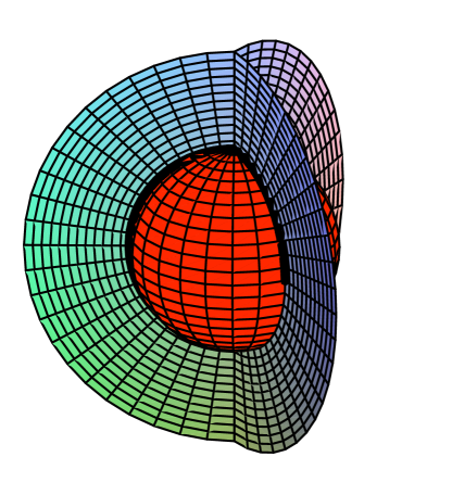
Figure 2: The subset of $\partial\Sigma$ where players $A$ and $B$ are indifferent, where we identify $\partial\Sigma$ with ${\mathbb{R}}^{3}\cup\{\infty\}$. Part of the periodic orbit $\tilde{\Gamma}$ is drawn as a fat curve. Another view of this periodic orbit is in Figure 3 (rotated 180 degrees about the $z$-axis).

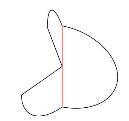
Figure 3: The periodic orbit $\tilde{\Gamma}$ in the Jitter set drawn in $\partial\Sigma$ where we identify $\partial\Sigma$ with ${\mathbb{R}}^{3}\cup\{\infty\}$. The vertical line is not part of the curve, but is drawn for clarity and because it forms the part where the four pieces from the global return section, introduced in Proposition 3.2 meet (the half-disc, and the two quarter discs, which meet along the vertical axis). The global return surface $S$ is the surface consisting of the half-disc, and two quarter discs meeting at the z-axis. The return section $Z$ mentioned in Theorem 3.1 is transversal to $\tilde{\Gamma}$ and so is not contained in $S$.

Remember that $\Sigma$ is a ball in ${\mathbb{R}}^{4}$ and $\partial\Sigma$ is homeomorphic to $S^{3}$. This set can be thought of as ${\mathbb{R}}^{3}\cup\{\infty\}$. Usually it is not easy to easy to give a geometric image of dynamics on $S^{3}$. But in fact, we are lucky. Instead of taking a section through a point $z\in\tilde{\Gamma}$ transversal to the periodic orbit $\tilde{\Gamma}$, we can find a set $S$ which is topologically a disc, such that $\partial S=\tilde{\Gamma}$, and such that orbits cross $S\setminus\tilde{\Gamma}$ transversally. This disc lies in the indifference sets. The subset of $\partial\Sigma$ where player $A$ is indifferent between strategies $i$ and $j$ is equal to $(\partial\Sigma_{A}\times Z_{ij}^{A})\cup(\Sigma_{A}\times(Z_{ij}^{A}\cap\partial\Sigma_{B}))$. This two-dimensional set is equal to a triangular tube together with a triangle at one end of the tube, in other words, it is homeomorphic to a topological disc. The boundary of this disc corresponds to the triangle $\partial\Sigma_{A}\times E^{B}$. Note that for each pair $i,j$ the boundary of this disc is the same. So if we identify $\partial\Sigma$ with ${\mathbb{R}}^{3}\cup\{\infty\}$, the set where player $A$ is indifferent between two strategies can be thought of as the union of the upper and lower part of the unit sphere in ${\mathbb{R}}^{3}$ (i.e. $\{(x,y,z)\,\,;\,\,x^{2}+y^{2}+z^{2}=1\mbox{ and }z\neq 0\}$) and the disc $\{(x,y,z)\,\,;\,\,x^{2}+y^{2}\leq 1\mbox{ and }z=0\}$. Similarly, the set where $B$ is indifferent can then be thought of as $\{(x,y,z)\,\,;\,\,(x,y)=(r\cos\phi,r\sin\phi)\mbox{ with }r\geq 0\mbox{ and }\phi=2\pi/3,4\pi/3,0\}\cup\{\infty\}$. The choice for $\phi$ represents which of the two strategies are indifferent for $B$. Again this represents three discs which all meet along the circle $\{(x,y,z)\,\,;\,\,x=y=0\}\cup\{\infty\}$ in ${\mathbb{R}}^{3}\cup\{\infty\}$. The orbit $\Gamma$ lies on the intersection of the sets where $A$ and $B$ are indifferent and is drawn in Figure 3. It turns out that one can find a subset $S$ of the space where player $A$ is indifferent, such that $\partial S=\tilde{\Gamma}$ and for which the orbits go through $S$ transversally.

Proposition 3.2.

There exists a topological disc $S$ in $\partial\Sigma$ with the following properties

• $S$ is a piecewise linear;

• $\partial S=\tilde{\Gamma}$;

• each orbit of the induced flow (except $\tilde{\Gamma}$) intersects $\tilde{\Gamma}$ transversally;

• the Poincaré return map to $S$ is a well-defined homeomorphism.

Proof.

Let $S$ consists of four pieces within the linear indifference sets $\Sigma_{A}\times Z^{A}_{i,j}$. These pieces are $U_{3}\times Z^{A}_{1,3}$, $U_{3}\times Z^{A}_{2,3}$, $U_{1}\times Z^{A}_{1,2}$, $U_{1}\times Z^{A}_{3,1}$, where $U_{i}$ is the part of $\Sigma_{A}$ where player $B$ prefers to head for corner $P_{i}^{A}$. The flow is transversal to each of these four linear sets. Also, inspection in the diagram of Figure 7 in Sparrow et al [2008] shows that no orbit can miss these sets (except if it is in $J$). The section $S$ forms a disc made up from the semi-disc and the two-half semi-discs depicted in Figure 3. ∎

Instead as in Figure 3, we can also visualise the section $S$ as in Figure 4. Indeed, $S\subset\partial\Sigma$ is made up of the following regions:

1. (the two triangles in $\Sigma_{A}$ where player $B$ heads for $1$ resp. $3$)   $\times$   (the point $R^{B}_{12}$);

2. (the part of $\partial\Sigma_{A}$ where player $B$ heads for $1$ resp. $3$)   $\times$   (the segment $[R^{B}_{12},E^{B}]$ in $\Sigma_{B}$);

3. (the part of $\partial\Sigma_{A}$ where player $B$ heads for $3$)   $\times$   (the segment $[R^{B}_{23},E^{B}]$ in $\Sigma_{B}$);

4. (the triangle $\Sigma_{A}$ where player $B$ heads for $3$)   $\times$   (the point $R^{B}_{23}$);

5. (the part of $\partial\Sigma_{A}$ where player $B$ heads for $1$)   $\times$   (the segment $[R^{B}_{31},E^{B}]$ in $\Sigma_{B}$);

6. (the part of $\Sigma_{A}$ where player $B$ heads for $1$)   $\times$   (the point $R^{B}_{23}$).

Using polar-like coordinates based at $E^{A}\in\Sigma_{A}$, the region 1 can be represented as an isosceles triangle (with, say, angles $80,50,50$). Attaching region 2 then gives a similar triangle (which is the bigger triangle in Figure 4). Joining all these regions together appropriately gives that $S$ can also be represented as in Figure 4. In this figure we also show an orbit of the first return map for $\beta=\sigma$ (the zero-sum case). The orbits, which tend to the Nash equilibrium in the full flow, do so in a rather chaotic fashion.

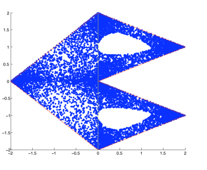
Figure 4: The orbit of a typical starting point under the first return map to $S$ when $\beta=\sigma$. The dynamics is similar to that of an area preserving map. There are two ’egg-shaped’ regions which are permuted by the first return map. Orbits within this region form invariant circles.

4 Dynamics for the original flow in $\Sigma$

Let us now state the implications of the results on the induced flow from the last section for the original flow.

4.1 Invariant cones

The implications of Theorem 3.1 for the real flow in $\Sigma_{A}\times\Sigma_{B}$ depend on the value of $\beta$, as described in the following proposition.

Proposition 4.1.

For the original flow the statements from Theorem 3.1 still hold in the following sense.

• For $\beta\in(0,\sigma)$ each periodic orbit $\gamma$ near $\tilde{\Gamma}$ of the induced flow, corresponds to an invariant cone $C(\gamma)$. Each orbit of the original flow starting in such a cone reaches the interior equilibrium in finite time (and then remains there).

• For $\beta\in(\sigma,1)$ periodic orbits near $\tilde{\Gamma}$ in $\partial\Sigma$ correspond to periodic orbits near $\Gamma$ on $J$. Thus there are infinitely many orbits of the flow in this parameter range. Moreover, there are orbits which jitter in the sense of the 2nd assertion of Theorem 3.1 and the flow contains a subshift of finite type, has positive topological entropy and has sensitive dependence on initial conditions.

Proof.

In Prop A2 in Sparrow et al [2008] it was shown that each orbit in $J$ tends to $E$ when $\beta\in(0,\sigma)$. In fact, on page 290 of that paper it was shown that if we take a section in $J$, then orbits converge exponentially fast to zero under iterates of the Poincaré map; moreover the time to spiral into the equilibrium $E$ is finite.

Now let $\tilde{V}$ be a plane in $\tilde{\Sigma}$ through a point $x_{0}\in\tilde{\Gamma}$ transversal to $\tilde{\Gamma}$ and $\tilde{R}$ be the first return map to $\tilde{V}$ corresponding to the induced flow. Identify $\Sigma$ with $\partial\Sigma\times[0,1]$ where $(x,0)\in\partial\Sigma\times[0,1]$ corresponds to $E$ and let $V=\tilde{V}\times[0,1]$. Let $R$ be the first return map to $V$ of the original flow. Then $R$ is of the form $R(x,t)=(\tilde{R}(x),\varrho_{x}(t))$. As we noted above, it was shown in Sparrow et al [2008] that $t\mapsto\varrho_{x}(t)$ has derivative less than one when $x=x_{0}$ and $\beta\in(0,\sigma)$. Note that

$$R^{n}(x,t)=(\tilde{R}^{n}(x),\varrho_{\tilde{R}^{n-1}(x)}\circ\dots\circ\varrho_{x}(t))$$

Since for $\beta\in(0,\sigma)$, $0$ is a hyperbolic attracting fixed point of $\varrho_{x_{0}}\colon{\mathbb{R}}^{+}\to{\mathbb{R}}^{+}$, if $\tilde{R}^{n}(x)=x$, $x\in\partial\Sigma$ and $x,\dots,\tilde{R}^{n-1}(x)$ are all sufficiently close to $x_{0}$ then $t\mapsto\varrho_{R^{n-1}(x)}\circ\dots\varrho_{x}(t)$ still has an attracting fixed point at $0$. So the periodic point $x$ for the induced flow corresponds to an orbit which tends towards the equilibrium point $E$ as $t\to\infty$ for the original flow. (Because of the parametrisation, orbits actually reach $E$ in finite time; during this time the orbit switches infinitely often between strategies.)

On the other hand, if $\beta\in(\sigma,1)$, then there exists a $t_{0}\in(0,1)$ so that $\Gamma\cap V$ corresponds to $(x_{0},t_{0})$. It was shown in Sparrow et al [2008] that $t_{0}$ is a hyperbolic attracting fixed point (and $0$ a repelling fixed point) of $\varrho_{z}\colon{\mathbb{R}}^{+}\to{\mathbb{R}}^{+}$, where $t_{0}>0$ is so that $\tilde{z}=(z,t_{0})\in\Gamma$. So if the periodic point $T^{n}(x)=x$ is sufficiently close to $z$ then $t\mapsto\varrho_{T^{n-1}(x)}\circ\dots\circ\varrho_{x}(t)$ still has an attracting fixed point $t$ near $t_{0}$. It follows that to each periodic point $x$ of the induced flow is associated a periodic point $(x,t)$ of the Poincaré return map of the flow (of the same period). In the same way one can prove that there are invariant sets which correspond to the second and third assertions of Theorem 3.1. ∎

5 Proof of Theorem 3.1

5.1 A geometric description of the flow near the Jitter set

..............................................................................................................................................................................................................................................................................................................................................................................................................................................................................................................................................................................................................................................................................................................................................................................................................................................................................................................................................................................................................................................................................................................................................................................................................................................................................................................................................................................................................................................................................................................................................................................................................................................................................................................................................................................................................................................................................................................................................................................................................................................................................................................................................................................................................................................................................................................................................$S$...................................................................................................................................................................................................................................................................................................................................................................................................................................................................................................................................................................................................................................................................................................................................................................................................................................................................................................................................................................................................................................................................................................................................................................................................................................................................................................................................................................................................................$*$$*$$*$$*$$*$$*$$z_{0}$$z$${\mathbb{Q}}_{z}$$W$$L$$*$$*$$*$$*$$\tilde{z}$...................................................................................................................................................................................................................................................................................................................................................................................................${\mathbb{Q}}$$C({\mathbb{Q}}_{z})$$\bullet$$\bullet$$\bullet$$\bullet$$T$...................................................................................................................................................................................................

Figure 5: The targets $P^{A}_{i},P^{A}_{j},P^{B}_{k},P^{B}_{l}$ in the plane $S$ are drawn marked as $\bullet$. The dashed line corresponds to $Z$. A quadrangle ${\mathbb{Q}}$ in $S$ is also drawn and also another quadrangle ${\mathbb{Q}}_{z}=\mbox{pr}^{-1}({\mathbb{Q}})\cap S_{0}$ which is in the plane $S_{0}\ni z_{0}$. The cone of the quadrangle with apex $T$ is invariant under the flow. In the figure we have taken the case that $d_{i}^{a}$ and $d_{i}^{b}$ are equal to $1$.

Before doing a rather cumbersome explicit calculation in the next subsection (for the game under consideration), we first want to explain geometrically what the dynamics near $Z^{*}$ looks like. As before let $Z^{\prime}=Z^{B}_{k,l}\times Z^{A}_{i,j}$ be a codimension-two plane where both players are indifferent between two strategies. In this section we consider the situation that near part of this set where both players are indifferent, both players choose repeatedly the strategies in a period four pattern $(i,k),(i,l),(j,l),(j,k)$. Let $S$ be the two-dimensional plane spanned by $[P^{A}_{i},P^{A}_{j}]\times[P^{B}_{k},P^{B}_{l}]\subset\Sigma_{A}\times\Sigma_{B}$. The orbit segments aim to the four targets in $S$, but an orbit which starts in $Z^{\prime}$ remains in $Z^{\prime}$ and aims for the point $T:=S\cap Z^{\prime}$. We call this point the cone-target. The linear (affine) spaces $S$ and $Z^{\prime}$ are of complementary dimensions and transverse. Let $L$ be a line through the cone-target $T$ contained in $Z^{\prime}$, and let $W$ be the three dimensional space $W=S+L$. Take $z_{0}\in L$, and assume that on some neighbourhood $U\subset W$ of $z_{0}$, the players only choose the above strategies. In other words, $U\setminus Z^{\prime}$ consists of four components, $S_{st}$ where $s\in\{i,j\}$ and $t\in\{k,l\}$ such that players $A$ and $B$ aim for $P_{s}^{A}$ resp. $P_{t}^{B}$ in $S_{st}$. First we prove that each orbit in $U$ lies within a cone with apex $T$ (the cone-target) induced over some quadrangles ${\mathbb{Q}}$, see Figure 5.

Let us define these quadrangles ${\mathbb{Q}}$. To do this, it is convenient apply a translation to $S\subset\Sigma_{A}\times\Sigma_{B}$ which puts $T=S\cap Z^{\prime}$ as the origin $(0,0)$ of $S\subset{\mathbb{R}}^{2}$ and identifies $S=[P_{i}^{A},P_{j}^{A}]\times[P_{k}^{B},P_{l}^{B}]$ with a rectangle in ${\mathbb{R}}\times{\mathbb{R}}$ so that $(P^{A}_{i},P^{B}_{k})$, $(P^{A}_{i},P^{B}_{l})$, $(P^{A}_{j},P^{B}_{l})$ and $(P^{A}_{j},P^{B}_{k})$ correspond to $(-d^{a}_{1},d^{b}_{1}),(-d^{a}_{1},-d^{b}_{2}),(d^{a}_{2},-d^{b}_{2}),(d^{a}_{2},d^{b}_{1})$ for some $d^{a}_{1},d^{a}_{2},d^{b}_{1},d^{b}_{2}\neq 0$ with $d^{a}_{1}d^{a}_{2}>0$ and $d^{b}_{1}d^{b}_{2}>0$. (The signs of $d^{a}_{1},d^{a}_{2},d^{b}_{1},d^{b}_{2}$ depend on whether the orbits flow clockwise or anticlockwise along $L$.) Now let ${\mathbb{Q}}$ be the quadrangle with corners

$$(d^{a}_{2},0),(0,\frac{d^{a}_{2}}{d^{a}_{1}}d^{b}_{1}),(-\frac{d^{b}_{1}}{d^{b}_{2}}d^{a}_{2},0),(0,-d^{b}_{1})$$ (5.5)

(or a multiple of it). Note that the four corners of this quadrangle lie on the coordinate axes and the sides of this quadrangle are parallel with the vector pointing from $O$ to $(P_{s}^{A},P_{t}^{B})$ in the region $\hat{S}_{st}$ corresponding to the projection of $S_{st}$ along the direction $L$. The quadrangle ${\mathbb{Q}}$ is shown in Figure 5.

Next take a plane $S_{0}\subset W$ through $z_{0}$ transversal to $L$ and take the projection $\mbox{pr}\colon S_{0}\to S$ along $L$. Furthermore, take $z\in S_{0}$, take the multiple $\epsilon{\mathbb{Q}}$ of the quadrangle ${\mathbb{Q}}$ in $S$ which contains $\mbox{pr}(z)\in S$ and define a quadrangle ${\mathbb{Q}}_{z}=\mbox{pr}^{-1}(\epsilon{\mathbb{Q}})\cap S_{0}$, see Figure 5. Each $z\in S_{0}$ sufficiently close to $z_{0}$ is contained in some quadrangle ${\mathbb{Q}}_{z}$ in this way. These quadrangles in $S_{0}$ have the following two property: (1) their corners are contained in two lines in $S_{0}$ which are orthogonal to each other and (2) the quadrangles are self-similar (they are all scalings of each other around the common ‘centre point’ $z_{0}$).

The reason these quadrangles are important is the following: Consider the cone $C({\mathbb{Q}}_{z})$ over ${\mathbb{Q}}_{z}$ with as apex the cone-target $T$. Since the ’vertical’ sides of this cone are contained in planes through the cone-target $T$ and the targets $(P^{A}_{s},P^{B}_{t})$, for each $z$ in this side the vector pointing from $z$ to $(P^{A}_{s},P^{B}_{t})$ is contained in the side of the cone. It follows that orbits which start in $C({\mathbb{Q}}_{z})$ remain in $C({\mathbb{Q}}_{z})$ until such time as one or both of the players start to play a third strategy.

......................................................................................................................................................................................$z_{0}$$q$$z$${\mathbb{Q}}$.........................................................................................................................................................................................................................................................................................................................................................................................................................................................................................................................................................................................................................................................................................................................................................................................................................................................................................................................................................................................................................................................................................................................

Figure 6: Arbitrary quadrangles can be mapped to standard quadrangles $\{(x,y)\in{\mathbb{R}}^{2};|x|+|y|=r\}$ by piecewise linear maps. An arc $\gamma$ connecting one of the corners of ${\mathbb{Q}}$ to some point $z\in{\mathbb{Q}}$ is also drawn (with dotted points). The angle of $z$ is equal to the $l(\gamma)/l({\mathbb{Q}})$ where $l$ is the usual Euclidean length in ${\mathbb{R}}^{2}$.

So consider such a family ${\mathbb{Q}}$ of quadrangles. Let us define a natural metric in $S_{0}$ associated to these quadrangles in the following way. The family ${\mathbb{Q}}$ of quadrangles can be mapped to the standard family of quadrangles $\{(x,y)\in{\mathbb{R}}^{2};|x|+|y|=r\}$ by a map $L$ which restricted to each quadrant is linear, see Figure 6 and with $L(z_{0})=0$. Thus we can define for each $z\in S_{0}$,

$$||z||_{S_{0}}=||Lz||$$

where $||\cdot||$ is the sum-norm on ${\mathbb{R}}^{2}$: if $w=(x,y)$ then $||w||=|x|+|y|$. So $||z_{0}||_{S_{0}}=0$ and the set $\{w\in S_{0};||w||_{S_{0}}=r\}$ is exactly a quadrangle from the above family. By analogy to the usual polar coordinates, we can associate an angle to $z\in S_{0}\setminus\{z_{0}\}$ in the following way. Pick one of the corners $q$ of the quadrangle ${\mathbb{Q}}=\{w\in S_{0};||w||_{S_{0}}=r\}$ where $r=||z||_{S_{0}}$, let $\gamma$ be the curve on this quadrangle which connects $q$ to $z$ (anti-clockwise). Then define $\phi(z)=2\pi\dfrac{l(\gamma)}{l({\mathbb{Q}})}$ where $l$ stands for the usual Euclidean length in ${\mathbb{R}}^{2}$. Thus we have defined quadrilateral polar coordinates $(r,\phi)$ of $z\in S_{0}\setminus\{z_{0}\}$ as follows:

$$r:=||z||_{S_{0}}\mbox{ and }\phi=2\pi\dfrac{l(\gamma)}{l({\mathbb{Q}})}$$

where ${\mathbb{Q}}=\{w\in S_{0};||w||_{S_{0}}=r\}$ and $r=||z||_{S_{0}}$. (This is completely analogous to how the usual polar coordinates are defined.)

Proposition 5.1 (Poincaré transition map for two planes parallel to $S$.).

Take two points $z_{0},z_{0}^{\prime}\in L$ so that along the segment $[z_{0},z_{0}^{\prime}]$ no other strategy becomes preferential (or indifferent) to the strategies $i,j$ for $A$ and $k,l$ for $B$. Let $S_{0},S_{0}^{\prime}$ be two-dimensional planes in $W$ through $z_{0}$ resp. $z_{0}^{\prime}$ which are both transversal to $L$. For $z\in S_{0}$ consider the quadrangle ${\mathbb{Q}}_{z}$ in $S_{0}$ constructed above and let $C({\mathbb{Q}}_{z})$ be the cone of ${\mathbb{Q}}_{z}$ over the cone-target $T$. Let $R(z)$ be the Poincaré map from $S_{0}$ to $S_{0}^{\prime}$. Then $R(z)$ is well-defined for $z$ close to $z_{0}$ and is contained in $C({\mathbb{Q}}_{z})\cap S_{0}^{\prime}$. Moreover, consider polar coordinates in the plane $S_{0}^{\prime}$ with the distance and angle taken from the point $S_{0}^{\prime}\cap L$. Then one can take a continuous map

$$\Psi\colon S_{0}\setminus\{z_{0}\}\ni z\mapsto{\mathbb{R}}$$

so that for each $z\in S_{0}\setminus\{z_{0}\}$ the value of $\Psi(z)$ modulo $2\pi$ is equal to the quadrilateral polar angle of $R(z)\in S_{0}\setminus\{z_{0}^{\prime}\}$ (as defined above). Then $\Psi(z)$ is equal to

$$2\pi\cdot\frac{1-c(z)}{a\cdot c(z)\cdot r}+B(z)+B_{0}.$$ (5.6)

Here $r:=||z||_{S_{0}}$, $c(z)$ is equal to $c_{0}(1+O(r))$ where $c_{0}=\mbox{\rm dist}(z_{0},T)/\mbox{\rm dist}(z_{0}^{\prime},T)\in(0,1)$ and where $O(r)$ is a function with $O(r)/r$ bounded as $r\to 0$,    $B(z)\colon S_{0}\setminus\{z_{0}\}\to{\mathbb{R}}$ is continuous function on $S_{0}$ with $B(z)\to 0$ as $z\to z_{0}$, and $B_{0}\in{\mathbb{R}}$ and $a>0$ are constants. Here dist is the usual Euclidean norm on the line $L$.

So the angle of $R(z)$ increases very fast as $r=||z||_{S_{0}}$ tends to zero.

..........................................................$l_{1}$$l_{2}$$l_{3}$$l_{4}$$\bullet$$\bullet$$\bullet$$\bullet$................................................................................................................................................................................................................................................................................................................................................................................................................................................................................................................................................................................................................................................................................................................................................................................................................................................................................................................................................................$l_{1}$$l_{2}$$l_{3}$$l_{4}$$\bullet$$\bullet$$\bullet$$\bullet$................................................................................................................................................................................................................................................................................................................................................................................................................................................................................................

Figure 7: The spiral motion in $S$ and the half-lines $l_{i}$ emanating from the centre $O$. The transition map from some quadrangle ${\mathbb{Q}}$ to $c_{0}{\mathbb{Q}}$ is also drawn.

Proof.

The only thing we need to prove is that (5.6) holds. To do this, note that the vector field is the product of a vector field in a direction along $L$ and one in the direction parallel to $S$. If we ignore the direction along $L$, then we get a new two-dimensional vector field on $S$ which corresponds to a two-dimensional game with spiral behaviour, see Figure 7. In other words, if we define $\mbox{pr}\colon W\to S$ to be the (linear) projection along $L$ and let $(z,t)\mapsto\Psi_{t}(z)$ be the flow through $z$, then pr projects the orbits of this flow in $W$ to orbits of a two-dimensional system in $S$. Moreover ${\mathbb{Q}}_{z}=\mbox{pr}({\mathbb{Q}}_{\tilde{z}})$ is a quadrangle in $S$ as defined above, where $\tilde{z}:=\mbox{pr}(z)\in S$. Denote the flow of this two-dimensional system through $\tilde{z}$ by $(\tilde{z},t)\mapsto\tilde{\Phi}_{t}(\tilde{z})$. Consider the piece $[0,A]\ni t\mapsto\Phi_{t}(z)$ of the orbit through $z\in S_{0}$ until it hits $S_{0}^{\prime}$. Then $[0,A]\ni t\mapsto\tilde{\Phi}_{t}(\tilde{z})$ is an arc with $\tilde{z}\in{\mathbb{Q}}_{\tilde{z}}$ and $\tilde{R}(\tilde{z})\in c(z)\cdot{\mathbb{Q}}_{\tilde{z}}$ where $c(z)>0$ is equal to $c_{0}(1+O(\mbox{\rm dist}(z,z_{0})))$ where

$$c_{0}:=\mbox{\rm dist}(S_{0}^{\prime}\cap L,O)/\mbox{\rm dist}(S_{0}\cap L,O)$$

and $O(x)$ is a function so that $O(x)/x$ is bounded when $x\to 0$. This holds because the angle between the ’vertical sides’ of $C({\mathbb{Q}}_{z})$ and $L$ tends to zero as $z\in S$ tends to $z_{0}$. (In fact, if $S_{0}$ and $S_{0}^{\prime}$ are both parallel to $S$ then $c(z)$ is exactly $c_{0}$.)

So it suffices to consider the projected flow $\tilde{\Phi}_{t}(\tilde{z})$ on $S$. That is, let us consider the Poincaré transition map $\tilde{R}$ which assigns to a point $\tilde{z}\in{\mathbb{Q}}_{\tilde{z}}\subset S$ the intersection of $c_{0}{\mathbb{Q}}_{\tilde{z}}$ with the orbit $t\mapsto\tilde{\Phi}_{t}(\tilde{z})$. Next consider the quadrilateral polar coordinates in $S$ (with the origin centered at $O$) and let $t\mapsto\phi_{t}(\tilde{z})$ be the angle of $\tilde{\Phi}_{t}(\tilde{z})$ (where we choose $t\mapsto\phi(\tilde{z})$ continuous). Then the angular change $\phi_{A}(\tilde{z})-\phi_{0}(\tilde{z})$ is equal to the $2\pi$ times the integer number of times the $[0,A]\ni t\mapsto\tilde{\Phi}_{t}(\tilde{z})$ winds around $O$ plus some number in $[0,2\pi]$. To compute this integer number of winding, consider the four half-line $l_{i}$ through the equilibrium $E_{S}$ of the two-dimensional game in $S$ where one of the players is indifferent and the other player always prefers one strategy, and denote these by $l_{m}$, $m=1,\dots,4$ (numbered so the flow meets these half-lines periodically in this order). Given $x\in l_{m}$, let $f_{m}(x)$ be the first time the flow meets $l_{m+1\mod{4}}$. Let us identify these lines with $[0,1]$ where $0$ corresponds to the equilibrium $E_{S}$. Since going from $l_{m}$ to $l_{m+1}$ is just the stereographic projection from $l_{m}$ to $l_{m+1}$ through lines of the target in the next region, $f_{m}(x)$ is of the form

$$r\mapsto\frac{r}{1+a_{m}r}\mbox{ with }m=1,2,3,4$$

where $r$ stands for the distance to the origin measured in the metric $||\cdot||_{S}$ (if, instead, we take the Euclidean metric then we get these maps are of the form $r\mapsto\frac{\theta_{m}r}{1+a_{m}r}$ where $\theta_{m}$ is related to the shape of the quadrangle). Since the composition of two Moebius transformations of the form $r\mapsto r/(1+\varrho_{1}r)$ and $r\mapsto r/(1+\varrho_{2}r)$ is equal to $x\mapsto r/(1+(\varrho_{1}+\varrho_{2})r$, we get that the Poincaré first return map $f$ to $l_{1}$ is of the form

$$f(r)=f_{4}\circ f_{3}\circ f_{2}\circ f_{1}(r)=\frac{r}{1+ar}\mbox{ where }a=a_{1}+a_{2}+a_{3}+a_{4}.$$

Hence $f^{n}(r)=\frac{r}{1+nar}$ for all $n$. So let $n$ be maximal so that $f^{n}(r)\geq cr$ where $c$ is equal to the number $c(z)$ from above. Then $n$ is the maximal integer so that $r/(1+nar)\geq c\cdot r$, i.e.,

$$n\leq\frac{1}{ar}\left(\frac{1-c}{c}\right).$$

In fact, $\phi(\tilde{R}(\tilde{z}))-\phi(\tilde{z})$ is constant for $z\in{\mathbb{Q}}$, because the relative length of an arc in ${\mathbb{Q}}$ (as a proportion of total perimeter length of ${\mathbb{Q}}$) is preserved under one central projections, see Figure 8 and therefore also under a composition of such maps. So in particular if $c_{0}$ is equal to $1/(1+nar)$ then the angle of $\tilde{R}(\tilde{z})$ and $\tilde{z}$ are the same modulo $2\pi$. If $1/(1+(n+1)car)<c_{0}<1/(1+ncar)$ then the result follows from a simple geometric consideration, see Figure 8. Thus we have proved Proposition 5.1. ∎

....................................................................................................................................................................................................................................................................................................................................................................................................................................................................................................................................................................................$c{\mathbb{Q}}$${\mathbb{Q}}$$\bullet$............................................$\gamma_{c}$...................................................................................................................................................................................................................................................................................................................................................................................................................................................................................................................................................................................................................................................................................................................................................................................................................................................................................................................................................................................................................................................................................................................................................................................................................................................................

Figure 8: Relative length (i.e. quadrilateral angle) is preserved by central projection. Moreover, let ${\mathbb{Q}}=\{z;||z||_{S}=r\}$. Then the length of the arc $\gamma_{c}$ between the vertical axis and the intersection of the line with $c{\mathbb{Q}}$ is equal to $(1-c)\theta r$ whereas the length of ${\mathbb{Q}}$ is equal to $\sqrt{2}cr$, where $\theta$ is a constant. So the angle of $\gamma_{c}$ is equal to $(1-c)\theta/(\sqrt{2}c)$ (plus a constant).

Note that after $n=[1/r]$ iterates of the map $f$ one has $f^{n}(r)=\frac{r}{1+nar}\approx c_{1}r$ where $c_{1}\in(0,1)$ is equal to $1/(1+a)$. During this time, the orbit has spiraled $n$ times around $O$ with each spiral between $T_{r}$ and $T_{c_{1}r}$. The length (and so the time-length) of the two-dimensional orbit is roughly $n\cdot c_{2}r\approx c_{2}$. Hence in one unit of time, the flow moves a point $\tilde{z}$ a definite factor closer to $O$.

5.2 An analytic computation of the flow near the Jitter set

$\beta>0$.....................................................................................................................................................................................................................................................................................................................................................................................................................................................................................................................................................................................................................................................................................................................................................................................................................................................................................................................................***$\bullet$$\bullet$$\bullet$$f_{12}^{A}$$f_{31}^{A}$$f_{23}^{A}$$R_{12}^{A}$$R_{31}^{A}$$R_{23}^{A}$$Q^{A}_{12}$$Q^{A}_{23}$$Q^{A}_{31}$$P^{A}_{1}$$P^{A}_{3}$$P^{A}_{2}$$2$$3$$1$.............................................................................................................................................................................................................................................................................................................................................................................................................................................................................................................................................................................................................................................................................................................................................................................................................................................................................................................................................................................................................................................................................................***$\bullet$$\bullet$$\bullet$$f_{31}^{B}$$f_{23}^{B}$$f_{12}^{B}$$R_{31}^{B}$$R_{23}^{B}$$R_{12}^{B}$$Q^{B}_{31}$$Q^{B}_{12}$$Q^{B}_{23}$$P^{B}_{1}$$P^{B}_{3}$$P^{B}_{2}$$1$$2$$3$...............................................................................................................................................

Figure 9: The simplices $\Sigma_{A}$ and $\Sigma_{B}$. The closed curve $\Gamma$ travels in both triangles clockwise along the three legs. $\Gamma$ reverses at the points $f^{A}_{ij}$ and $f^{B}_{ij}$.

In this section we will make some precise calculations for the periodic orbit $\tilde{\Gamma}$ on the Jitter set for the induced flow on $\partial\Sigma$. More precisely, we will consider the first return map to some first return section at some point in $\Gamma$. To do this, consider the line $V_{0}$ in $\Sigma_{A}$ where player $B$ is indifferent between strategies $2$ and $3$ (it goes from $R^{A}_{23}$ to $Q^{A}_{23}$, see Figure 9 for the location of these points). Similarly, let $V_{1}$ in $\Sigma_{B}$ be where player $A$ is indifferent between strategies $2$ and $3$ (it goes from $R^{B}_{23}$ to $Q^{B}_{23}$) and let $V_{2}$ be the line in $\Sigma_{A}$ where player $B$ is indifferent between strategies $1$ and $3$ (it goes from $R^{A}_{31}$ to $Q^{A}_{31}$). Moreover, let $\partial\Sigma_{A}^{ij}$ be the side of $\partial\Sigma_{A}$ containing $R^{A}_{ij}$ and similarly define $\partial\Sigma_{B}^{ij}$ as the side of $\partial\Sigma_{B}$ containing $R^{B}_{ij}$ .

Let $R_{0}$ be the first entry map $V_{0}\times\partial\Sigma_{B}^{31}\to\partial\Sigma_{A}^{12}\times V_{1}$ and $R_{1}$ be the first entry map $\partial\Sigma_{A}^{12}\times V_{1}\to V_{2}\times\partial\Sigma_{B}^{12}$ corresponding to the induced flows on $\partial\Sigma$. By the symmetry of the system, the first return map to $V_{0}\times\partial\Sigma_{B}^{31}$ is equal to the third iterate of $R_{1}\circ R_{0}$. (Provided we make sure we choose the axis consistently.)

The first leg of the orbit $\Gamma$ (the one which is contained in $Z_{1,2}^{B}\times Z_{1,3}^{B}\subset\Sigma_{A}\times\Sigma_{B}$ and which is the first piece of the two legs of the orbit $\Gamma$ shown in Figure 9) corresponds to the first entry map $R_{0}$. During the transition which corresponds to $R_{0}$, player $A$ only chooses between strategy $1$ and $3$ and player $B$ only chooses between strategy $2$ and $1$. Note that as soon as the orbit hits $\Sigma_{A}\times V_{1}$ and until it hits $V_{2}\times\Sigma_{B}$, player $A$ will only choose between strategies $1$ and $2$ (while player $B$ still only plays $1$ and $2$). So the first entry maps to these sections allow us to consider the pieces of the orbit where each players only switch between two strategies.

Let us describe how much further or closer an orbits near $\tilde{\Gamma}$ can get to $\tilde{\Gamma}$ while it orbits nearby. To do this, define the sum-distance (i.e. the metric dist) on $\partial\Sigma\subset\Sigma\subset{\mathbb{R}}^{6}$ between two points $z=(z_{1},\dots,z_{6})$, $w=(z_{1},\dots,w_{6})$ by

$$\mbox{\rm dist}(z,w)=\sum_{i=1,\dots,6}\,\,|z_{i}-w_{i}|.$$

This metric is well-suited to dealing with quadrilaterals. Because of the discussion in the previous subsection, there exist quadrilaterals in $V_{0}\times\partial\Sigma_{B}^{13}$ which are mapped by $R_{1}$ into another quadrilaterals in $\partial\Sigma_{A}^{12}\times V_{1}$ (and similarly for $R_{2}$). Let us compute these quadrilaterals (up to first order). It will be important to be consistent in the choice so let us write

$$V_{0}\times\partial\Sigma_{B}^{13}=[R^{A}_{23},Q_{23}^{A}]\times[P_{1}^{B},P_{3}^{B}],$$

$$\partial\Sigma_{A}^{12}\times V_{1}=[P_{1}^{A},P_{3}^{A}]\times[Q^{B}_{23},R^{B}_{23}],$$

$$V_{2}\times\partial\Sigma_{B}^{21}=[R^{A}_{31},Q^{A}_{31}]\times[P_{2}^{B},P_{1}^{B}]$$

and number the half-lines clockwise starting with the positive horizontal axis, see Figure 10.

..............................................................................................................................................................................................................................................................................................$R^{A}_{23}$$Q^{A}_{23}$$P_{1}^{B}$$P_{3}^{B}$$1$$4$$3$$2$..............................................................................................................................................................................................................................................................................................$P_{1}^{A}$$P_{3}^{A}$$Q^{B}_{23}$$R^{B}_{23}$$1$$4$$3$$2$..............................................................................................................................................................................................................................................................................................$1$$4$$3$$2$$R^{A}_{31}$$Q^{A}_{31}$$P_{2}^{B}$$P_{1}^{B}$

Figure 10: The first return map to $[R^{A}_{23},Q_{23}^{A}]\times[P_{1}^{B},P_{3}^{B}]$ is equal to the third iterate of $R_{1}\circ R_{0}$ provided we identify $[R^{A}_{31},Q^{A}_{31}]\times[P_{2}^{B},P_{1}^{B}]$ with $[R^{A}_{23},Q_{23}^{A}]\times[P_{1}^{B},P_{3}^{B}]$ in a consistent way. For this reason we order the half-lines in the coordinate axis in the return sections as shown. The origins of these axes are $(E^{A},R^{B}_{31})$, $(R^{A}_{12},E^{B})$ and $(E^{A},R^{B}_{12})$.

Proposition 5.2.

For each $\epsilon>0$ small, there exists a quadrilateral ${\mathbb{Q}}_{V_{0},R_{0}}^{\epsilon}\subset V_{0}\times\partial\Sigma_{B}^{13}$ with corners in the coordinate axes, and such that the sum-distance of corners (1),(2),(3),(4) (labeled as in Figure 10 on the left) to $(E^{A},R^{B}_{13})$ are equal, up to terms of order $\epsilon^{2}$, to

$$\frac{2}{3}\frac{(2+\beta)\epsilon}{1+\beta+\beta^{2}},\,\,\frac{2\epsilon}{(2-\beta)(1+\beta)},\,\,\frac{2}{3}\frac{(2+\beta)\epsilon}{\beta(1+\beta+\beta^{2})},\,\,\frac{2\epsilon}{2-\beta}.$$ (5.7)

Similarly there exists a quadrilateral ${\mathbb{Q}}_{V_{1},R_{0}}^{\epsilon}\subset\partial\Sigma_{A}^{12}\times V_{1}$ with corners in the coordinate axes, and such that the sum-distance of these corners (1),(2),(3),(4) (labeled as in Figure 10 in the middle) to $(R^{A}_{12},E^{B})$ are equal, up to terms of order $\epsilon^{2}$, to

$$\begin{array}[]{rl}&\dfrac{2(2-\beta)\epsilon}{(1+\beta)(2+\beta)},\\ &\\ &\dfrac{2}{3}\dfrac{(4-4\beta+\beta^{2})\epsilon}{1+\beta^{3}+\beta+\beta^{4}}\mbox{ for }\beta\in(0,1/2)\mbox{ and }\dfrac{2}{3}\dfrac{(2-\beta)\epsilon}{1+\beta^{3}}\mbox{ for }\beta\in(1/2,1),\\ &\\ &\dfrac{2(2-\beta)\epsilon}{\beta(1+\beta)(2+\beta)},\\ &\\ &\dfrac{2}{3}\dfrac{(4-4\beta+\beta^{2})\epsilon}{(1+\beta^{3})}\mbox{ for }\beta\in(0,1/2)\mbox{ and }\dfrac{2}{3}\dfrac{(2-\beta)\epsilon}{1-\beta+\beta^{2}}\mbox{ for }\beta\in(1/2,1).\end{array}$$ (5.8)

The first entry map $R_{0}$ maps $Q_{V_{0},R_{0}}^{\epsilon}$ into $Q_{V_{1},R_{0}}^{\epsilon}$.

...................................................................................................................................................................................................................................................................................................................................................................................................................................................................................................................................................................................................................................................................................................................................................................................................................................................................................................$*$...............................................................$R_{12}^{A}$$R_{31}^{A}$$R_{23}^{A}$$Q^{A}_{12}$$Q^{A}_{23}$$Q^{A}_{31}$$P^{A}_{1}$$P^{A}_{3}$$P^{A}_{2}$$2$$3$$1$...................................................................................................................................................................................................................................................................................................................................................................................................................................................................................................................................................................................................................................................................................................................................................................................................................................................................................................$R_{23}^{B}$$R_{12}^{B}$$Q^{B}_{31}$$Q^{B}_{12}$$Q^{B}_{23}$$P^{B}_{1}$$P^{B}_{3}$$P^{B}_{2}$$1$$2$$3$$*$.....................................

Figure 11: The simplices $\Sigma_{A}$ and $\Sigma_{B}$. The line $V_{0}\subset\Sigma^{A}$ is drawn in the left triangle and the line $V_{1}\subset\Sigma^{B}$ on the right, and the first four line segments of the orbit (starting at time $t_{0}=0$ at the point $*$) which are computed in the proof of Proposition 5.2 are shown.

So this proposition gives precise information on how much further or closer one gets to $\tilde{\Gamma}$ during the transition from $V_{0}\times\partial\Sigma_{B}^{13}$ to $\partial\Sigma_{A}^{12}\times V_{1}$. Remember that we saw in the previous subsection that the angle of $R_{0}(z)$ depends extremely sensitively on $\epsilon$ and so it essentially suffices to compare the size of the terms in (5.7) to those in (5.7).

What we need to do in the proof of Proposition 5.2 is to associate to $R_{0}$ invariant cones as in the previous subsection, and the corresponding quadrangles in $V_{0}\times\partial\Sigma_{B}^{13}$ and in $\partial\Sigma_{A}^{12}\times V_{1}$. After that, we will do the same for the first entry map $R_{1}$.

Proof.

Since we want to consider the induced flow on $\partial\Sigma$, we take a starting point $(p^{A},p^{B})\in V_{0}\times\partial\Sigma_{B}^{12}$ when considering the map $R_{0}$. During this part of the orbit, the orbit jitters around this first leg of $\Gamma$. To describe this precisely, we explicitly compute the quadrilateral from the previous subsection. As we have seen in the previous subsection the orbit is contained in a cone with apex the ’cone-target’ which in this case is equal to $(T_{A},T_{B})=(R^{A}_{12},Q_{13}^{B})$. To compute this cone, let us take as a special starting point in $V_{0}\times\partial\Sigma_{B}^{13}$ the point $p_{A}=(1/3,1/3,1/3),p_{B}=(1-\beta-\epsilon,0,1+\epsilon)/(2-\beta)$ (where $p_{B}=R^{B}_{13}$ when $\epsilon=0$) and compute the first four pieces where this orbit aims for $(P_{3}^{A},P_{1}^{B})$, $(P_{1}^{A},P_{1}^{B})$, $(P_{1}^{A},P_{2}^{B})$ and $(P^{A}_{3},P^{B}_{2})$ under the original flow (i.e. the first four times when the players hit an indifference plane under the original flow). Since the calculations are rather laborious and it is easy to make a mistake, we did this by using Maple (the worksheet can be requested from the authors - and also is available on the first author’s webpage). For simplicity we take the parametrisation $p^{A}(t_{k}+s)=p^{A}(t_{k})(1-s)+sP^{A}_{i}$ and $p^{A}(t_{k}+s)=p^{A}(t_{k})(1-s)+sP^{A}_{j}$ for all $t\in(t_{k},t_{k+1})$ provided $A$ resp. $B$ aim for $P^{A}_{i},P^{B}_{j}$ during this time interval. The first hitting time is at $\hat{t}_{1}:=t_{1}:=\epsilon/(1+\epsilon)$, and then

$$p_{A}(\hat{t}_{1})=\left(\dfrac{1}{3(1+\epsilon)},\dfrac{1}{3(1+\epsilon)},\dfrac{1+3\epsilon}{3(1+\epsilon)}\right)\mbox{ , }\quad p_{B}(\hat{t}_{1})=\left(\frac{1-\beta}{2-\beta},0,\frac{1}{2-\beta}\right).$$

The next time the players hit an indifference plane is at $\hat{t}_{2}:=t_{1}+t_{2}$ where $t_{2}:=\epsilon/(\beta+\beta\epsilon+1+2\epsilon)$ and then

$$p_{A}(\hat{t}_{2}):=\left(\dfrac{1}{3}\dfrac{\epsilon+\beta+1}{\beta+\beta\,\epsilon+1+2\,\epsilon}\,\,,\,\,\dfrac{1}{3}\dfrac{\beta+1}{\beta+\beta\,\epsilon+1+2\,\epsilon}\,\,,\,\,\dfrac{1}{3}\dfrac{\left(1+3\,\epsilon\right)\left(\beta+1\right)}{\beta+\beta\,\epsilon+1+2\,\epsilon}\right),$$

$$p_{B}(\hat{t}_{2}):=\left(\frac{{\beta}^{2}+{\beta}^{2}\epsilon-1-3\,\epsilon+\beta\,\epsilon}{\left(\beta+\beta\,\epsilon+1+2\,\epsilon\right)\left(-2+\beta\right)}\,\,,\,\,0\,\,,\,\,-\frac{\beta+\beta\,\epsilon+1+\epsilon}{\left(\beta+\beta\,\epsilon+1+2\,\epsilon\right)\left(-2+\beta\right)}\right)$$

Then it hits at $\hat{t}_{3}:=t_{1}+t_{2}+t_{3}$ with $t_{3}:=\epsilon/({\beta}^{2}+{\beta}^{2}\epsilon+\beta+2\,\beta\,\epsilon+\epsilon)$ and then $p_{A}(\hat{t}_{3})$ and $p_{B}(\hat{t}_{3})$ are equal to

$$\left(\dfrac{1}{3}\frac{\beta+3\,\epsilon}{\beta+\beta\,\epsilon+\epsilon}\,\,,\,\,\frac{1}{3}\dfrac{\beta}{\beta+\beta\,\epsilon+\epsilon}\,\,,\,\,\dfrac{1}{3}\frac{\beta\,\left(1+3\,\epsilon\right)}{\beta+\beta\,\epsilon+\epsilon}\right)\,\,,$$

$$\left(\frac{\left({\beta}^{2}+{\beta}^{2}\epsilon-1-3\,\epsilon+\beta\,\epsilon\right)\beta}{\left(-2+\beta\right)\left({\beta}^{2}+{\beta}^{2}\epsilon+\beta+2\,\beta\,\epsilon+\epsilon\right)}\,\,,\,\,\frac{\epsilon}{{\beta}^{2}+{\beta}^{2}\epsilon+\beta+2\,\beta\,\epsilon+\epsilon}\,\,,\,\,-\frac{\left(1+\epsilon\right)\beta}{\left(-2+\beta\right)\left(\beta+\beta\,\epsilon+\epsilon\right)}\right)$$

and again at $\hat{t}_{4}:=\hat{t}_{3}+t_{4}$ where $t_{4}:=\epsilon/(\beta+\beta\epsilon+2\epsilon)$ and then $p_{A}(\hat{t}_{4})$ and $p_{B}(\hat{t}_{4})$ are

$$\left(\frac{1}{3}\frac{\beta+3\,\epsilon}{\beta+\beta\,\epsilon+2\,\epsilon}\,\,,\,\,\frac{1}{3}\frac{\beta}{\beta+\beta\,\epsilon+2\,\epsilon}\,\,,\,\,\frac{1}{3}\frac{\beta+3\,\beta\,\epsilon+3\,\epsilon}{\beta+\beta\,\epsilon+2\,\epsilon}\right),$$

$$\left(\frac{\beta\,\left({\beta}^{2}+{\beta}^{2}\epsilon-1-3\,\epsilon+\beta\,\epsilon\right)}{\left(\beta+1\right)\left(-2+\beta\right)\left(\beta+\beta\,\epsilon+2\,\epsilon\right)}\,\,,\,\,\frac{\left(\beta+2\right)\epsilon}{\left(\beta+1\right)\left(\beta+\beta\,\epsilon+2\,\epsilon\right)}\,\,,\,\,-\frac{\beta\,\left(1+\epsilon\right)}{\left(-2+\beta\right)\left(\beta+\beta\,\epsilon+2\,\epsilon\right)}\right).$$

Next we compute the cone. As mentioned, the cone-targets are

$$T_{A}:=\left(\frac{1}{\beta+2}\,\,,\,\,0\,\,,\,\,\frac{\beta+1}{\beta+2}\right)\mbox{ and }T_{B}:=\left(\frac{\beta}{\beta+1}\,\,,\,\,\frac{1}{\beta+1}\,\,,\,\,0\right)$$

and we compute the intersection of the line through $(T_{A},T_{B})$ and the points $(p_{A}(\hat{t}_{i}),p_{B}(\hat{t}_{i}))$, $i=1,\dots,4$ with the three-dimensional section $V_{0}\times\Sigma_{B}$. This gives an intersection point at $\hat{t}_{1}$,

$$\left(1/3\frac{-3\,\beta\,\epsilon+{\beta}^{2}+\beta+1}{{\beta}^{2}+\beta-\beta\,\epsilon+1+\epsilon}\,\,,\,\,1/3\frac{{\beta}^{2}+\beta+1}{{\beta}^{2}+\beta-\beta\,\epsilon+1+\epsilon}\,\,,\,\,1/3\frac{{\beta}^{2}+\beta+1+3\,\epsilon}{{\beta}^{2}+\beta-\beta\,\epsilon+1+\epsilon}\right),$$

$$\left(\frac{{4\beta}^{2}\epsilon+{\beta}^{4}+{\beta}^{3}+{\beta}^{3}\epsilon-\beta-1-\beta\,\epsilon-\epsilon}{\left({\beta}^{2}+\beta-\beta\,\epsilon+1+\epsilon\right)\left(\beta+1\right)\left(-2+\beta\right)}\,\,,\,\,-\frac{\beta\,\epsilon\,\left(\beta+2\right)}{\left({\beta}^{2}+\beta-\beta\,\epsilon+1+\epsilon\right)\left(\beta+1\right)}\,\,,\,\,\right.$$

$$\left.-\frac{\left({\beta}^{2}+\beta+1\right)\left(1+\epsilon\right)}{\left({\beta}^{2}+\beta-\beta\,\epsilon+1+\epsilon\right)\left(-2+\beta\right)}\right);$$

at $\hat{t}_{2}$ the intersection point is

$$(1/3,1/3,1/3),$$

$$\left(\frac{2\,\beta\,\epsilon+{\beta}^{3}+{\beta}^{2}+2\,{\beta}^{2}\epsilon-\beta-1-3\,\epsilon}{\left(\beta+1\right)^{2}\left(-2+\beta\right)}\,\,,\,\,-{\frac{\epsilon\,\left(\beta+2\right)}{\left(\beta+1\right)^{2}}}\,\,,\,\,-\frac{1+\epsilon}{-2+\beta}\right);$$

at $\hat{t}_{3}$ the intersection point is

$$\left(1/3\frac{\left({\beta}^{2}+\beta+1+3\,\epsilon\right)\beta}{{\beta}^{2}+\beta+{\beta}^{3}+\beta\,\epsilon-\epsilon}\,\,,\,\,1/3\frac{\left({\beta}^{2}+\beta+1\right)\beta}{{\beta}^{2}+\beta+{\beta}^{3}+\beta\,\epsilon-\epsilon}\,\,,\,\,1/3\frac{{\beta}^{3}+{\beta}^{2}+\beta-3\,\epsilon}{{\beta}^{2}+\beta+{\beta}^{3}+\beta\,\epsilon-\epsilon}\right)$$

$$\left(\frac{\beta\,\left({\beta}^{4}+2\,{\beta}^{3}\epsilon+{\beta}^{3}+2\,{\beta}^{2}\epsilon-2\,\beta\,\epsilon-\beta+\epsilon-1\right)}{\left(\beta+1\right)\left(-2+\beta\right)\left({\beta}^{2}+\beta+{\beta}^{3}+\beta\,\epsilon-\epsilon\right)}\,\,,\,\,-\frac{\epsilon\,\left({\beta}^{3}+{\beta}^{2}+1\right)}{\left({\beta}^{2}+\beta+{\beta}^{3}+\beta\,\epsilon-\epsilon\right)\left(\beta+1\right)}\,\,,\,\,\right.$$

$$\left.-\frac{\left({\beta}^{2}+\beta+1\right)\left(1+\epsilon\right)\beta}{\left({\beta}^{2}+\beta+{\beta}^{3}+\beta\,\epsilon-\epsilon\right)\left(-2+\beta\right)}\right)$$

while at $\hat{t}_{4}$ the intersection point we get is the original starting point (this is not surprising because the orbit lies on the cone through these points):

$$\left(1/3,1/3,1/3\right)\mbox{ , }\left(\frac{1-\beta}{2-\beta},0,\frac{1}{2-\beta}\right).$$

These four points in $\Sigma_{A}\times\Sigma_{B}$ together with the apex $(T_{A},T_{B})$ determine a cone (for each $\epsilon>0)$.

However, remember we want to compute the cone for the induced flow. This means that we have to take the intersection of the lines from $(E^{A},E^{B})$ through these points with $\partial\Sigma$. Since $\epsilon>0$ is small, these points will be contained in $V_{0}\times\partial\Sigma_{B}^{13}$. This gives at $\hat{t}_{1}$,

$$\left(1/3\frac{{\beta}^{3}+2\,{\beta}^{2}+2\,\beta+1+3\,\beta\,\epsilon}{{\beta}^{3}+2\,{\beta}^{2}+2\,\beta+2\,{\beta}^{2}\epsilon+1+\epsilon+6\,\beta\,\epsilon}\,\,,\,\,1/3{\frac{{\beta}^{3}+2\,{\beta}^{2}+2\,\beta+3\,{\beta}^{2}\epsilon+1+6\,\beta\,\epsilon}{{\beta}^{3}+2\,{\beta}^{2}+2\,\beta+2\,{\beta}^{2}\epsilon+1+\epsilon+6\,\beta\,\epsilon}}\,\,,\,\,\right.$$

$$\left.1/3\frac{{\beta}^{3}+2\,{\beta}^{2}+2\,\beta+3\,{\beta}^{2}\epsilon+1+3\,\epsilon+9\,\beta\,\epsilon}{{\beta}^{3}+2\,{\beta}^{2}+2\,\beta+2\,{\beta}^{2}\epsilon+1+\epsilon+6\,\beta\,\epsilon}\right)$$

$$\left(\frac{-1+\beta}{-2+\beta}\,\,,\,\,0\,\,,\,\,\frac{1}{2-\beta}\right)$$

at $\hat{t}_{2}$,

$$\left(1/3,1/3,1/3\right),$$

$$\left(\frac{{\beta}^{3}-\beta-1+3\,{\beta}^{2}\epsilon-7\,\epsilon+2\,\beta\,\epsilon+{\beta}^{2}}{\left({\beta}^{2}+2\,\beta+1+3\,\beta\,\epsilon+6\,\epsilon\right)\left(-2+\beta\right)}\,\,,\,\,0\,\,,\,\,-\frac{2\,\beta+1+5\,\epsilon+{\beta}^{2}+2\,\beta\,\epsilon}{\left({\beta}^{2}+2\,\beta+1+3\,\beta\,\epsilon+6\,\epsilon\right)\left(-2+\beta\right)}\right)$$

at $\hat{t}_{3}$,

$$\left(1/3\frac{2\,{\beta}^{3}+2\,{\beta}^{2}+\beta+{\beta}^{4}+6\,{\beta}^{2}\epsilon+3\,\epsilon+3\,{\beta}^{3}\epsilon+3\,\beta\,\epsilon}{2\,{\beta}^{3}+2\,{\beta}^{2}+\beta+{\beta}^{4}+4\,{\beta}^{2}\epsilon+2\,\epsilon+3\,{\beta}^{3}\epsilon}\,\,,\,\,1/3\frac{2\,{\beta}^{3}+2\,{\beta}^{2}+\beta+{\beta}^{4}+3\,{\beta}^{2}\epsilon+3\,\epsilon+3\,{\beta}^{3}\epsilon}{2\,{\beta}^{3}+2\,{\beta}^{2}+\beta+{\beta}^{4}+4\,{\beta}^{2}\epsilon+2\,\epsilon+3\,{\beta}^{3}\epsilon}\,\,,\,\,\right.$$

$$\left.1/3\frac{\beta\,\left(2\,{\beta}^{2}+2\,\beta+1+{\beta}^{3}+3\,\beta\,\epsilon+3\,{\beta}^{2}\epsilon-3\,\epsilon\right)}{2\,{\beta}^{3}+2\,{\beta}^{2}+\beta+{\beta}^{4}+4\,{\beta}^{2}\epsilon+2\,\epsilon+3\,{\beta}^{3}\epsilon}\right)$$

$$\left(\frac{1-\beta}{2-\beta}\,\,,\,\,0\,\,,\,\,\frac{1}{2-\beta}\right)$$

and at $\hat{t}_{4}$ again the point we started with

$$\left(1/3,1/3,1/3\right)\,\,,\,\,\left(\frac{\beta+\epsilon-1}{-2+\beta}\,\,,\,\,0\,\,,\,\,\frac{1-\epsilon}{-2+\beta}\right).$$

These four points determine a quadrangle ${\mathbb{Q}}^{\epsilon}_{V_{0},R_{0}}$ in $V_{0}\times\partial\Sigma_{B}^{13}$.

Next we find the intersection points of these cones with $\Sigma_{A}\times V_{1}$ and then take the intersections with $\partial\Sigma$ of half-lines from $E$ in the direction of these points. Since the expressions are rather similar to the ones before, we will only give these final points in $\partial\Sigma_{B}\times V_{1}$. The intersection corresponding to $\hat{t}_{1}$ is

$$\left(\frac{\beta+\beta\,\epsilon+1+\epsilon}{\left(3\,\epsilon+\beta+1\right)\left(\beta+2\right)}\,\,,\,\,0\,\,,\,\,\frac{2\,\beta+1+5\,\epsilon+{\beta}^{2}+2\,\beta\,\epsilon}{\left(3\,\epsilon+\beta+1\right)\left(\beta+2\right)}\right)\,\,,\,\,\left(1/3,1/3,1/3\right),$$

to $\hat{t}_{2}$ is

$$\left(\frac{1}{\beta+2}\,\,,\,\,0\,\,,\,\,\frac{\beta+1}{\beta+2}\right),$$

$$\left(1/3\frac{3\,{\beta}^{2}\epsilon-9\,\beta\,\epsilon+1+9\,\epsilon+{\beta}^{3}+3\,{\beta}^{3}\epsilon+\beta+{\beta}^{4}}{2\,{\beta}^{2}\epsilon-5\,\beta\,\epsilon+1+5\,\epsilon+{\beta}^{3}+3\,{\beta}^{3}\epsilon+\beta+{\beta}^{4}}\,\,,\,\,1/3\frac{3\,{\beta}^{2}\epsilon-6\,\beta\,\epsilon+1+3\,\epsilon+{\beta}^{3}+3\,{\beta}^{3}\epsilon+\beta+{\beta}^{4}}{2\,{\beta}^{2}\epsilon-5\,\beta\,\epsilon+1+5\,\epsilon+{\beta}^{3}+3\,{\beta}^{3}\epsilon+\beta+{\beta}^{4}}\,\,,\,\,\right.$$

$$\left.1/3\frac{1+{\beta}^{3}+\beta+{\beta}^{4}+3\,\epsilon+3\,{\beta}^{3}\epsilon}{2\,{\beta}^{2}\epsilon-5\,\beta\,\epsilon+1+5\,\epsilon+{\beta}^{3}+3\,{\beta}^{3}\epsilon+\beta+{\beta}^{4}}\right),$$

to $\hat{t}_{3}$,

$$\left(\frac{2\,\beta\,\epsilon+{\beta}^{2}+\beta+2\,\epsilon}{\left(3\,\epsilon+\beta+1\right)\beta\,\left(\beta+2\right)}\,\,,\,\,0\,\,,\,\,\frac{3\,{\beta}^{2}\epsilon+4\,\beta\,\epsilon+{\beta}^{3}+2\,{\beta}^{2}+\beta-2\,\epsilon}{\left(3\,\epsilon+\beta+1\right)\beta\,\left(\beta+2\right)}\right)\,\,,\,\,\left(1/3,1/3,1/3\right),$$

and to $\hat{t}_{4}$,

$$\left(\frac{1}{\beta+2}\,\,,\,\,0\,\,,\,\,\frac{\beta+1}{\beta+2}\right),$$

$$\left(1/3\frac{6\,\beta\,\epsilon+1-3\,\epsilon+{\beta}^{3}}{2\,\beta\,\epsilon+1+\epsilon+{\beta}^{2}\epsilon+{\beta}^{3}}\,\,,\,\,1/3\frac{{\beta}^{2}-\beta+1+3\,\epsilon}{{\beta}^{2}-\beta+\beta\,\epsilon+1+\epsilon}\,\,,\,\,1/3\frac{1+{\beta}^{3}-3\,\beta\,\epsilon+3\,\epsilon+3\,{\beta}^{2}\epsilon}{2\,\beta\,\epsilon+1+\epsilon+{\beta}^{2}\epsilon+{\beta}^{3}}\right).$$

These points form the quadrilaterals ${\mathbb{Q}}_{V_{1},R_{0}}^{\epsilon}$ in $\partial\Sigma_{B}^{12}\times V_{1}$.

To get Proposition 5.2 we differentiate the points forming the quadrilaterals ${\mathbb{Q}}_{V_{0},R_{0}}^{\epsilon}$ and ${\mathbb{Q}}_{V_{1},R_{0}}^{\epsilon}$ with respect to $\epsilon$. Since these points correspond to probability vectors, the sum of these derivatives is equal to zero. So we merely need to take the sum of the absolute values of these derivatives (or twice the positive terms).

∎

Since the calculations from $R_{1}$ are similar to those done in the Proposition 5.2 we shall not show them here. The maple worksheet in which these computations are done can be obtained from the authors on request.

...................................................................................................................................................................................................................................................................................................................................................................................................................................................................................................................................................................................................................................................................................................................................................................................................................................................................................................$R_{12}^{A}$$R_{31}^{A}$$R_{23}^{A}$$Q^{A}_{12}$$Q^{A}_{23}$$Q^{A}_{31}$$P^{A}_{1}$$P^{A}_{3}$$P^{A}_{2}$$2$$3$$1$$*$........................................................................................................................................................................................................................................................................................................................................................................................................................................................................................................................................................................................................................................................................................................................................................................................................................................................................................................................................$R_{23}^{B}$$R_{12}^{B}$$Q^{B}_{31}$$Q^{B}_{12}$$Q^{B}_{23}$$P^{B}_{1}$$P^{B}_{3}$$P^{B}_{2}$$1$$2$$3$$*$.........................................

Figure 12: The simplices $\Sigma_{A}$ and $\Sigma_{B}$. The line $V_{1}\subset\Sigma^{B}$ is drawn in the right triangle and the line $V_{2}\subset\Sigma^{A}$ on the left, and the first four line segments of the orbit (starting at time $t_{0}=0$ at the point $*$) which are computed in the proof of Proposition 5.2 are shown. Notice that $t_{1},t_{2},t_{3},t_{4}$ correspond to half-lines (2), (3), (4), (1) in the middle of Figure 10 and to (4), (1), (2), (3) on the right. This can be seen by taking the cones through the target points, intersect them respectively with $\Sigma^{A}\times V_{1}$ and $V_{2}\times\Sigma^{B}$, and then project from $E$ on the boundary of $\Sigma$.

Proposition 5.3.

For each $\epsilon>0$ small, there exists a quadrilateral ${\mathbb{Q}}_{V_{1},R_{1}}^{\epsilon}\subset\partial\Sigma_{A}^{12}\times V_{1}$ with corners in the coordinate axes, and such that the sum-distance of these corners (1),(2),(3),(4) (labeled as in Figure 10) to $(R^{B}_{12},E^{B})$ are equal, up to terms of order $\epsilon^{2}$, to

$$\begin{array}[]{rl}&\dfrac{2\epsilon}{2+\beta}\\ &\\ &\dfrac{2}{3}\dfrac{(2-3\beta+\beta^{2})\epsilon}{1+\beta^{3}}\mbox{ for }\beta\in(0,1/2)\mbox{ and }\dfrac{2}{3}\dfrac{1-\beta}{1-\beta+\beta^{2}}\mbox{ for }\beta\in(1/2,1),\\ &\\ &\dfrac{2(1-\beta)\epsilon}{2+\beta},\\ &\\ &\dfrac{2}{3}\dfrac{(2-3\beta+\beta^{2})\epsilon}{\beta(1-\beta+\beta^{2})}\mbox{ for }\beta\in(0,1/2)\mbox{ and }\dfrac{2}{3}\dfrac{(1-\beta^{2})\epsilon}{\beta(1-\beta+\beta^{2})}\mbox{ for }\beta\in(1/2,1)\end{array}$$ (5.9)

Similarly there exists a quadrilateral ${\mathbb{Q}}_{V_{2},R_{1}}^{\epsilon}\subset V_{2}\times\partial\Sigma_{B}^{12}$ with corners in the coordinate axes, and such that the sum-distance of these corners (1),(2),(3),(4) (labeled as in the figure on the right in Figure 10) corners to $(E^{A},R^{A}_{12})$ are equal, up to terms of order $\epsilon^{2}$, to

$$\begin{array}[]{rl}&\dfrac{2}{3}\dfrac{(4-3\beta^{2}-\beta^{3})\epsilon}{1+3\beta+3\beta^{2}+2\beta^{3}},\,\,\dfrac{2(2-\beta-\beta^{2})\epsilon}{(1+2\beta)(2-\beta)\beta},\\ &\\ &\quad\dfrac{2}{3}\dfrac{(11+21\beta+15\beta^{2}+7\beta^{3})\epsilon}{(1+3\beta+3\beta^{2}+2\beta^{3})(2+\beta)},\,\,\dfrac{2(2-\beta-\beta^{2})\epsilon}{(1+2\beta)(1+\beta)(2-\beta)}.\end{array}$$ (5.10)

The first entry map $R_{1}$ maps $Q_{V_{1},R_{1}}^{\epsilon}$ into $Q_{V_{2},R_{1}}^{\epsilon}$.

5.3 The dynamics of a Jitter map

The dynamics near the periodic orbit $\Gamma$ is very complicated. As we have seen, the Poincaré transition map to a section at a point of $\Gamma$ is a composition of maps of the following form:

$$x\mapsto A_{1}\circ R_{2\pi/||y||+B(y)}\circ A_{0}^{-1}(x)\mbox{ where }y=A_{0}^{-1}(x).$$

In this section we shall first study the iterations of one of these maps. In the next section we will then consider the composition of two suitable Jitter maps.

Let dist be a metric on ${\mathbb{R}}^{2}$ with the property that each half-line through the origin intersects $\partial D_{r}$ in a unique point (where $D_{r}:=\{z\in{\mathbb{R}}^{2};\,|z|:=\mbox{\rm dist}(z,0)=r\}$). Next take $R_{t}\colon{\mathbb{R}}^{2}\to{\mathbb{R}}^{2}$ to be the quadrilateral rotation, i.e. the unique map so that ${\mathbb{R}}^{2}\times{\mathbb{R}}\ni(z,t)\mapsto R_{t}(z)\in{\mathbb{R}}^{2}$ is continuous, $R_{0}=id$, so that for each $z\in{\mathbb{R}}^{2}$, $\mbox{\rm dist}(R_{t}(z),0)=\mbox{\rm dist}(z,0)$ and so that for each $x\in{\mathbb{R}}^{2}\setminus\{0\}$ the angles of $R_{t}(z)$ and $z$ differ by $t$. If dist is the Euclidean metric then this coincides with the usual rotation, but in our setting it is convenient to take for dist the sum-metric on ${\mathbb{R}}^{2}$ (defined by $\mbox{\rm dist}(z,z^{\prime}):=||z-z^{\prime}||:=|x-x^{\prime}|+|y-y^{\prime}|$ for $z=(x,y)$ and $z^{\prime}=(x^{\prime},y^{\prime})$) in which case $t\mapsto R_{t}(z)$ moves each point along a square $\partial D_{r}(0)$.

Next define two homeomorphisms $A_{0},A_{1}\colon{\mathbb{R}}^{2}\to{\mathbb{R}}^{2}$ which preserve the axes and which map quadrilaterals containing $0$ with corners on the axes to quadrilaterals of the form $\partial D_{r}=\{(x,y)\in{\mathbb{R}}^{2}\,;\,\,|x|+|y|=r\}$. Assume that there exist $\lambda<1<\mu$ so that for each $t\in(\lambda,\mu)$ there exists a smooth curve $l_{t}$ through $0$ so that

$$\mbox{\rm dist}(A_{0}^{-1}\circ A_{1}(z),0)=t\cdot\mbox{\rm dist}(z,0)\mbox{ for each }z\in l_{t}$$ (5.11)

and such that $A_{0}^{-1}A_{1}(l_{t})$ is transversal to $\partial D_{r}$ for each $r>0$. Consider

$$F(z)=A_{1}\circ R_{\theta(w)}\circ A_{0}^{-1}(z)$$

where

$$\theta(w)=2\pi/||w||+B(w)\mbox{ , }w=A_{0}^{-1}(z)\mbox{ and }||w||=\mbox{\rm dist}(w,0)$$

and $w\mapsto B(w)\in{\mathbb{R}}$ is a continuous function which converges to zero as $w\to 0$. We will refer to $F$ as a ‘jitter map’.

Let us prove that such a Jitter map maps are ’chaotic’.

Proposition 5.4 (A jitter map has many periodic orbits).

Let $F$ be as above and assume (5.11). Then the map $F$ has periodic orbits of arbitrary period in each neighbourhood of $0$.

Proposition 5.5 (A jitter map contains a shift with infinitely many symbols).

Let $F$ be as above and assume (5.11). Then there exists $N_{0}$ so that for each sequence $k_{i}\in{\mathbb{N}}$ satisfying

$$\lambda\leq\dfrac{k_{i+1}}{k_{i}}\leq\mu\mbox{ with }k_{i}\geq N_{0}$$

there exist a sequence $\delta_{i}\in(0,1)$ and $z\neq 0$ with $||F^{i}(z)||\in(\frac{1}{k_{i}+1+\delta_{i}},\frac{1}{k_{i}+\delta_{i}})$ for all $i\geq 0$.

Proposition 5.6.

Let $F$ be as above and assume (5.11). Then there exists $N_{0}$ so that for each sequence $k_{i}\in{\mathbb{N}}$ there exists a sequence $\delta_{i}\in(0,1)$ so that

$$\lambda\leq\dfrac{k_{i+1}}{k_{i}}\leq\mu\mbox{ and }k_{i}\geq N_{0}$$

there exists $z\neq 0$ with $||F^{i}(z)||\in(\frac{1}{k_{i}+1+\delta_{i}},\frac{1}{k_{i}+\delta_{i}})$ for all $i\geq 0$.

The first proposition implies, for example, that there is a sequence of fixed points of $F$ converging to $0$.

The second proposition implies that $F$ contains a shift on infinitely many symbols. Indeed, define the annuli

$$Ann_{k}:=\{z\in{\mathbb{R}}^{2};\dfrac{1}{(k+2)}\leq{||}z{||}\leq\dfrac{1}{k}\}.$$

The annuli with $k$ even are all disjoint. Hence, taking $k_{i}\in 2{\mathbb{Z}}$ in Proposition 5.5, we get the existence of $x\in Ann_{k_{0}}$ with $F^{i}(x)\in Ann_{k_{i}}$ for all $i$. If we would consider $k_{i}\in\{k_{0},k_{0}+2\}$ this would give a one-sided shift on two symbols, but the proposition guarantees the existence of orbits which jump several annuli further in or out (the number is determined by $\lambda$ and $\mu$). It follows that $F$ has positive topological entropy. In fact, the topological entropy is infinite because for each $n$, it contains a full one-sided shift of $n$ symbols (which has entropy $\log n$).

Corollary 5.1 (A jitter map has sensitive dependence on initial conditions).

Let $F$ be as above and assume (5.11). Then $F$ has sensitive dependence on initial conditions for all points in the set corresponding to the shift on infinitely many symbols.

..................................................................................................................................................................................................................................................................................................................................................................................................................................................................................................................................................................................................................................................................................................................................................................................................................................................................................................................................................................................................................................................................................................................................................................................................................................................................$l$.............................................................................................................................................................................................................................................................................................................................................................................................................................................................................................................................................................................................................................................................................................................................................................................................................................................................................................................................................................................................................................................................................................................................................................................................................................................................................................................................................................................................................................................................................................................................................................................................................................................................................................................................................................................................................................................................................................................................................................................................................................................................................................................................................................................................................................................................................................................................................................................................................................................................................................................................................................................................................................................................................................................................................................................................................................................................................................................................................................................................................................................................................................................................................................................................................................................................................................................................................................

Figure 13: On the left, the image of a curve $l$ through $0$ is a spiral. A conveniently chosen curve $l$ contains a sequence of fixed points, converging to $0$. On the right, the sequence of annuli discussed below the statement of Proposition 5.5. Orbits can jump between annuli according to these allowed sequences (5.5).

Proof of Proposition 5.4. Let us start by showing why $F$ has a sequence of fixed points tending to $0$. It will be convenient to consider

$$\hat{F}(y):=A\circ R_{\theta(y)}(y)\mbox{ where }A=A_{0}^{-1}\circ A_{1}.$$

By assumption there exists a curve $l$ through $0$ so that ${||}A(z){||}={||}z{||}$ for $z\in l$. Let $l_{+}$ be one of the two components of $l\setminus\{0\}$, let $l^{\prime}_{+}:=A(l_{+})$ and let $m_{+}:=A_{1}(l_{+})$. We shall find a sequence of fixed points $y$ of $F$ on $m_{+}\setminus\{0\}$. Indeed, for each $r>0$ small, let $\alpha(r)$ be the angle between the vectors $l_{r}^{\prime}O$ and $l_{r}O$ where $l_{r}^{\prime}\in l^{\prime}_{+}$ and $l_{r}\in l_{+}$ are the unique points so that $||l_{r}^{\prime}||=||l_{r}||=r$. Then choose $y\in l^{\prime}_{+}$ so that

$$\theta(y)=2\pi/||y||+B(y)=\alpha(||y||)\mod 2\pi.$$ (5.12)

Since $B(y)$ is bounded and continuous, there exists a sequence of such points on $l^{\prime}_{+}$ converging to $0$. More precisely, there exists $\alpha$ so that for each sufficiently large $k\in{\mathbb{N}}$ there exists $r\in(\frac{1}{k+1+\theta},\frac{1}{k+\theta})$ so that $y\in l^{\prime}_{+}$ with $|y|=r$ satisfied (5.12). So assume that (5.12) holds. Then for any such $y\in l^{\prime}_{+}$ the point $x:=A_{0}y\in m_{+}$ is a fixed point of $F$. Indeed, $R_{\theta(y)}(y)=R_{\alpha(|y|)}(y)\in l$ by the choice of $y$ and $\alpha$. So

$${||}\hat{F}(y){||}=||A\circ R_{\theta(y)}(y)||=||R_{\theta(y)}(y)||=||y||$$ (5.13)

and

$$A\circ R_{\theta(y)}(y)\in l^{\prime}.$$ (5.14)

Since $y\in l^{\prime}_{+}$ and $l^{\prime}_{+}$ is a smooth curve which is transversal to the quadrangles $D_{r}$, equations (5.13) and 5.14) implies that $\hat{F}(y)=A\circ R_{\theta(y)}(y)=y$. Hence $A_{0}\circ\hat{F}(y)=A_{0}(y)$ and so $F(x)=A_{0}\circ\hat{F}\circ A_{0}^{-1}(x)=x$ for $x=A_{0}(y)\in m_{+}$.

To explain the general case of periodic points of higher periods, let us show how to construct a periodic orbit of period three (the general case goes similarly). Consider the surface

$$\tilde{P}(3)=\{(a_{1},a_{2},a_{3})\,\,;\,\,a_{i}\in{\mathbb{R}}^{+}\mbox{ and }a_{1}a_{2}a_{3}=1\}.$$

Choose $a_{1},a_{2},a_{3}\in(\lambda,\mu)$ on this surface $\tilde{P}(3)$ and a disc neighbourhood $U$ of this point in this surface. Associate to $a=(a_{1},a_{2},a_{3})$ the curves $l_{i}$, $i=1,2,3$ through $0$ such that $||A(z)||=a_{i}||z||$ for all $z\in l_{i}$ and let $l_{i,+}$ be a component of $l_{i}\setminus\{0\}$. Let $l^{\prime}_{i,+}=A(l_{i,+})$. For each $r>0$, let $\alpha_{i}(r)$ be the angle between the $Ol^{\prime}_{i,r}$ and $Ol_{i+1,r}$ where $l^{\prime}_{i,r}=l^{\prime}_{i,+}\cap\partial D_{r}$ and $l_{i+1,r}=l_{i+1,+}\cap\partial D_{r}$ (and where we take $l_{3+1}=l_{1}$). Assume there exists $r>0$ and $a\in\tilde{P}(3)$ so that

$$\begin{array}[]{llll}\theta(l^{\prime}_{1,r})&=&\alpha_{1}(r)&\mod 2\pi\\ \theta(l^{\prime}_{2,a_{2}r})&=&\alpha_{2}(a_{2}r)&\mod 2\pi\\ \theta(l^{\prime}_{3,a_{2}a_{3}r})&=&\alpha_{3}(a_{2}a_{3}r)&\mod 2\pi.\end{array}$$ (5.15)

We claim that this implies that $x:=A_{0}(y)$ is a periodic point of $F$ of period three where $y=l_{1,r}$. Indeed, because $y=l_{1,r}=l^{\prime}_{1,+}\cap D_{r}$ the first equation from (5.15) implies that $R_{\theta(y)}(y)\in l_{2,+}$ and therefore that ${||}\hat{F}(y){||}={||}A\circ R_{\theta(y)}(y){||}=a_{2}{||}y{||}=a_{2}r$ and $\hat{F}(y)=A\circ R_{\theta(y)}(y)\in l_{2,+}^{\prime}$. This and the second equation from (5.15) implies that $R_{\theta(\hat{F}(x))}(\hat{F}(y))\in l_{3,+}$ and so ${||}\hat{F}\circ\hat{F}(y){||}={||}A\circ R_{\theta(\hat{F}(x))}(\hat{F}(y)){||}=a_{3}{||}|\hat{F}(y){||}=a_{2}a_{3}r$. Finally, this and the third equation from (5.15) implies that $R_{\hat{F}^{2}(y)}(\hat{F}^{2}(y))\in l_{1,+}$ and so $||\hat{F}^{3}(y)||=a_{1}a_{2}a_{3}||y||$ and $\hat{F}^{3}(y)\in l_{1,+}^{\prime}$. Because $a_{1}a_{2}a_{3}=1$ and both $\hat{F}^{3}(y)$ and $y$ are in $l_{1,+}^{\prime}$ we get therefore that $\hat{F}^{3}(y)=y$. Hence $F^{3}(x)=A_{0}\circ\hat{F}^{3}\circ A_{0}^{-1}(x)=x$.

So we need to show that (5.15) has solutions. Define $G\colon{\mathbb{R}}^{+}\times\tilde{P}(3)\to{\mathbb{R}}\times{\mathbb{R}}\times{\mathbb{R}}$ by

$$G(r,a_{1},a_{2},a_{3})=(\alpha_{1}(r),\alpha_{2}(a_{2}r),\alpha_{3}(a_{2}a_{3}r))$$

where $y\in l^{\prime}_{1,+}\cap D_{r}$ and $\alpha_{i}$ are the angles defined above. This map is continuous and bounded. In fact, for each $\epsilon>0$ there exist $\delta>0$ and a neighbourhood $U$ in $\tilde{P}(3)$ as above so that $G((0,\delta)\times U)$ is contained in $\epsilon$-ball in ${\mathbb{R}}^{3}$. Next define the map

$$H\colon{\mathbb{R}}^{+}\times\tilde{P}(3)\ni(r,a)\mapsto(\theta(l^{\prime}_{1,r}),\theta(l^{\prime}_{2,a_{2}r}),\theta(l^{\prime}_{3,a_{2}a_{3}r}))\in{\mathbb{R}}\times{\mathbb{R}}\times{\mathbb{R}}.$$

$H$ can be written as $H_{1}+H_{2}$ where

$$H_{1}(r,a)=(2\pi/r,2\pi/(a_{2}r),2\pi/(a_{2}a_{3}r))\,\,\mbox{ and }\,\,H_{2}(r,a)=(B(l^{\prime}_{1,r}),B(l^{\prime}_{2,a_{2}r}),B(l^{\prime}_{3,a_{2}a_{3}r})).$$

Note that (5.15) is equivalent to $G(r,a)=H(r,a)$, i.e. to $G(r,a)-H_{2}(r,a)=H_{1}(r,a)$ (modulo $2\pi$). The values of the left-side map $(0,\delta)\times U\ni(r,a)\mapsto G(r,a)-H_{2}(r,a)$ are contained in a $2\epsilon$-ball, provided we choose $\delta>0$ so small that $|B(y)|\leq\epsilon$ for all $y$ with ${||}y{||}\leq\delta$. Note that $H_{1}\colon(0,\delta)\times U\to{\mathbb{R}}^{3}$ is invertible and has inverse $H_{1}^{-1}(y_{1},y_{2},y_{3})=(2\pi/y_{1},y_{1}/y_{2},y_{2}/y_{3})$. Hence $H_{1}^{-1}$ maps $2\pi\underline{k}+[0,2\pi]^{3}$, $\underline{k}=(k_{0},k_{1},k_{2})\in{\mathbb{Z}}^{3}$ into $(0,\delta)\times U$ provided $|k_{i}|$ is large. So $(G-H_{2})\circ H_{1}^{-1}$ maps $2\pi\underline{k}+[0,2\pi]^{3}$ into some $2\epsilon$ ball. By Brouwer’s fixed point theorem, $(G-H_{2})\circ H_{1}^{-1}$ has a fixed point (modulo $2\pi$) in $2\pi\underline{k}+\underline{\kappa}_{0}+[0,2\pi]^{3}$ for some $\underline{\kappa}_{0}\in{\mathbb{R}}^{3}$ (where $\underline{k}$ is arbitrary but with $|k_{i}|$ large. Hence there exists a constant $\kappa$ so that for each $k_{0}$ large, $G(r,a)=H(r,a)$ (modulo $2\pi$) has a solution $(r,a)$ with $r\in(\frac{1}{k_{0}+1+\kappa},\frac{1}{k_{0}+\kappa})$ and $a\in U\subset\tilde{P}(3)$. ∎

Proof of Proposition 5.5. The proof of the second assertion also has a similar flavour, but to explain the proof more clearly we will assume that $B(z)=0$ and that the curve $l_{t}$ as in (5.11) are lines. Again write $\hat{F}=A^{-1}\circ F$ where $A=A^{-1}_{0}\circ A_{1}$. Assume that $k_{0},k_{1},\dots$ is a sequence as in the assumption of the proposition, and let $\kappa_{0},\kappa_{1},\dots\in(0,1)$ be a sequence to be determined later on. Take $U_{0}=(1/(k_{0}+\kappa+1),1/k_{0}+\kappa_{0})$ and inductively choose a sequence of intervals $U_{1},U_{2},\dots$ so that $U_{n}$ is the set of all $a_{n}\in{\mathbb{R}}$ so that for all $x\in U_{0}$ and all $a_{i}\in U_{i}$, $i=1,\dots,n-1$,

$$1/(a_{1}\dots a_{n}x)\in(k_{n}+\kappa_{n},k_{n}+\kappa_{n}+1).$$

Next let $l_{0}^{\prime}={\mathbb{R}}^{+}$ and for $i\geq 1$, let $l_{i}$ be the half-line in the positive quadrant with $||Ax||=a_{i}||x||$ on $l_{i}$. Define $l^{\prime}_{i}=Al_{i}$, $i\geq 1$ and for $i=0,1,2,\dots$ let $\alpha_{i}$ be the angle between $l^{\prime}_{i}$ and $l_{i+1}$. Note that $\alpha_{i}$ depends on $a_{i}$ and $a_{i+1}$.

We want to show that for each $n$ there exists a solution $x\in U_{1}$ and $a_{i}\in U_{i}$, $i=2,3,\dots$ of the system of equalities (analogous to (5.15)):

$$\begin{array}[]{rl}2\pi/x&=\alpha_{0}(a_{1})\mod 2\pi\\ 2\pi/(a_{2}x)&=\alpha_{1}(a_{1},a_{2})\mod 2\pi\\ &\vdots\\ 2\pi/(a_{n}\cdot\dots\cdot a_{3}a_{2}x)&=\alpha_{n-1}(a_{n-1},a_{n})\mod 2\pi.\end{array}$$ (5.16)

Let us show that this is enough. Take $x\in\l_{0}^{\prime}={\mathbb{R}}^{+}$ with distance $x$ to $0$. Assume that we have $\hat{F}^{i}(x)\in l_{i}^{\prime}$ and $||\hat{F}^{i}(x)||=a_{1}\dots a_{i}x$. Then the above equations give $R_{\theta(\hat{F}^{i}(x))}(\hat{F}^{i}(x))\in l_{i+1}$, $||\hat{F}^{i+1}(x)||=a_{i+1}{||}\hat{F}^{i}(x){||}=|a_{1}\cdots a_{i+1}x|$ for $i=0,1,\dots,n$ and $\hat{F}^{i+1}(x)\in l_{i+1}^{\prime}$. Since $x\in U_{0}$ and $a_{i}\in U_{i}$, $i=1,2,\dots$ this proves by induction that

$$||\hat{F}^{i}(x)||\in(\dfrac{1}{k_{i}+\delta_{i}+1},\dfrac{1}{k_{i}+\delta_{i}}).$$

for each $i=0,1,2,\dots$.

To prove that for each $n$ there exist $x\in U_{0}$ and $a_{i}\in U_{i}$ as in (5.16), let

$$H(x,a_{2},\dots,a_{n})=\left(2\pi/x,2\pi/(a_{2}x),\dots,2\pi/(a_{n}a_{n-1}\cdots a_{2}x)\right)$$

and

$$G(x,a_{2},\dots,a_{n})=(\alpha_{0}(a_{1}),\alpha_{1}(a_{1},a_{2}),\alpha_{2}(a_{2},a_{3}),\dots,\alpha_{n-1}(a_{n-1},a_{n})).$$

$H$ is invertible with

$$H^{-1}(y_{0},\dots,y_{n-1})=(2\pi/y_{0},y_{1}/y_{0},\dots,y_{n-1}/y_{n-2}).$$

Now take $\underline{k}=(k_{0},k_{1},\dots,k_{n-1})$ with $k_{i}\geq N_{0}$ and with $\lambda\leq k_{i+1}/k_{i}\leq\mu$. For each $\epsilon>0$ there exists $N_{0}$ so that $H^{-1}$ maps $2\pi\underline{k}+[-2\pi,4\pi]^{n}$ into some $\epsilon$-neighbourhood of $(k_{0},k_{1}/k_{0},\dots,k_{n-1}/k_{n-2})$. Then $G$ maps this neighbourhood into a neighbourhood of some point in ${\mathbb{R}}^{n}$. It follows that there exists $\underline{\kappa}=(\kappa_{0},\dots,\kappa_{n-1})\in{\mathbb{R}}^{n}$ so that $G\circ H^{-1}$ maps $2\pi\underline{k}+2\pi\underline{\kappa}+[0,2\pi]^{n}$ into itself, and therefore has a fixed point $(y_{0},\dots,y_{n-1})\in 2\pi\underline{k}+2\pi\underline{\kappa}+[0,2\pi]^{n}$. It follows $G=H$ (modulo $2\pi$) has as a solution $(x,a_{2},\dots,a_{n})=H(y_{0},\dots,y_{n-1})$ of the required form. ∎

5.4 The dynamics of the composition of two jitter maps and the Proof of Theorem 3.1

To prove Theorem 3.1 note that we have seen in Proposition 5.1 that the first entry maps $R_{0}$ and $R_{1}$ are of the form

$$x\mapsto A_{1}\circ R_{2\pi/||y||+B(y)}\circ A_{0}^{-1}(x)\mbox{ where }y=A_{0}^{-1}(x)$$

and

$$x\mapsto A_{3}\circ R_{2\pi/||y||+B^{\prime}(y)}\circ A_{2}^{-1}(x)\mbox{ where }y=A_{2}^{-1}(x).$$

The first return map to the section associated to $V_{0}$ is the third iterate of $R_{1}\circ R_{0}$ (provided we identify the target space of $R_{1}$ appropriately with the domain space of $R_{0}$, as we have done in the previous subsection, see for example Figure 10). To show that this map has the required properties, we proceed as in the proof of Proposition 5.4 and write

$$\hat{F}(x)=A_{0}^{-1}\circ A_{3}\circ R_{1/||y^{\prime}||+B^{\prime}(y^{\prime})}\circ A_{2}^{-1}\circ A_{1}\circ R_{1/||y||+B(y)}.$$

Note that $A_{i}$ is a piecewise linear map (linear on each quadrant), and so we can describe these by four parameters (which determine the position of each corner of the quadrilaterals). To compute the condition analogous to (5.11), for $A_{2}^{-1}\circ A_{1}$ we take the ratio of the $i$-th term in (5.8) to the $i$-th term in (5.9):

$$\frac{(2-\beta)}{(\beta+1)},\dfrac{(2-\beta)}{(1-\beta^{2})},\frac{(2-\beta)}{(\beta+1)\beta(1-\beta)},\frac{(2-\beta)\beta}{(1-\beta^{2})}.$$

The largest one of these (the third one) is $\geq 3.5$ for all $\beta\in(0,1)$ whereas the last one is $\leq 1$ for all $\beta\in(0,1/2)$ (it is increasing) and the first one is $\leq 1$ for all $\beta(1/2,1)$ (it is decreasing). So $|A_{2}^{-1}A_{1}(z)|/|z|$ can vary between $1$ and $3.5$.

To compute the condition analogous to (5.11), for $A_{3}^{-1}\circ A_{0}$ we take the ratio of the $i$-th term in (5.7) to the $i$-th term in (5.10):

$$\dfrac{(2-\beta-\beta^{2})}{(1+2\beta)},\dfrac{(2-\beta-\beta^{2})(1+\beta)}{(1+2\beta)\beta},\dfrac{\beta(11+21\beta+15\beta^{2}+7\beta^{3})}{(2+\beta)^{2}(1+2\beta)},\frac{(2-\beta-\beta^{2})}{(1+2\beta)(1+\beta)}.$$

The largest of these is either the 2nd or the 3rd, and the maximum of these two is $\geq 1.2$ for all $\beta\in(0,1)$. The third one is increasing and the last one increasing, with the first one $<0.8$ for $\beta\in(0,0.35)$ and the last one $<0.8$ for $\beta\in(0.35,1)$. So $|A_{0}^{-1}A_{3}(z)|/|z|$ can vary between $0.8$ and $3.5$.

So the condition corresponding to (5.11) holds. It follows that $\hat{F}$ has a sequence of fixed points (and periodic orbits) as before, and that the properties as in Theorem 3.1 hold.

6 Proof of Theorem 1.4.

Take matrices $A$ and $B$ with

$$||A-A_{\beta}||,||B-B_{\beta}||\leq\epsilon$$

where $||\,\,\,||$ stands for some matrix norm.

That the Shapley and anti-Shapley orbit exists for $A,B$ near $A_{\beta},B_{\beta}$, simply follows from the hyperbolicity of the first return map to a section transversal to these orbits. (The first return maps are projective transformations.)

So let us discuss the persistence of the orbit $\Gamma$. Provided $\epsilon>0$ is small enough, the set $\Sigma_{A}$ and $\Sigma_{B}$ are still divided up in three regions meeting in a Nash equilibrium as in Figure 1. (The angles between the lines will no longer be necessarily equal and the Nash equilibria will no longer be in the barycentre.) Now again consider the induced flow on the boundary. The set where one or two players are indifferent are still arranged as in Figures 2 and 3 (they change continuously with $A$ and $B$). The part of $\partial\Sigma$ where both players are indifferent still consists of a closed curve $\Gamma$ along which orbits spiral (along cones as in Figure 5), and the other part through which orbits cross transversally. The transition maps can be computed along this orbit as was done in Section 5.2, but in any case, the quadrangles computed in that section depend again continuously on $A$ and $B$. So it follows that for fictitious play associated to $A$ and $B$ sufficiently close to $A_{\beta},B_{\beta}$, one still has the existence of a sequence of periodic orbits for the flow induced on the boundary.

Next we argue for the original system. The cone over the hexagonal $\Gamma$ with apex the Nash equilibrium $E$ is completely invariant and depends continuously on $A,B$. Moreover, this cone is two dimensional (but of course embedded in the four-dimensional space $\Sigma$). So now take a half-line $l$ in this cone through the apex, and consider the first return map to $l$. Because of the general form of the return maps, this first return map $R\colon l\to l$ is a Moebius transformation, with a fixed point at $E$. As we showed in the appendix of Sparrow et al [2008], taking $A_{\beta},B_{\beta}$ we have the following: for $\beta\in(0,\sigma)$ the fixed point $E$ of $R\colon l\to l$ is attracting, for $\beta=\sigma$ it is neutral, and for $\beta\in(\sigma,1)$ repelling and another fixed point appears which attracts all points in $l\setminus\{E\}$, because the map is a Moebius map. (For $\beta\in(0,\sigma)$, the map $R\colon l\to l$ also has a ’virtual’ 2nd fixed point, corresponding to the ’negative’ part of the half-line $l$.) For $A,B$ close to $A_{\beta},B_{\beta}$ the corresponding first return maps are also near those of $A_{\beta},B_{\beta}$. So when $\beta\neq\sigma$, and $A,B$ is sufficiently close to $A_{\beta},B_{\beta}$ we have the same behaviour for $\Gamma$.

Using Proposition 4.1 one can get the same conclusions for the other periodic orbits for the original flow.

7 Conclusion

For $\beta\in(-1,0]$ players always asymptotically become periodic. When $\beta\in(0,\sigma)$ the Shapley orbit is still attracting but not globally attracting: there is an abundance of orbits (many with periodic play) as described in Theorem 1.1 which tend to $E$. For $\beta\in(\sigma,1)$ we have chaos (in the sense that there exist subshifts of finite type). This chaos is caused by a periodic orbit $\Gamma$ whose first return map is of what we call ‘jitter type’: orbits can move further away and closer to the periodic orbit $\Gamma$ in a manner which is reminiscent to that of a random walk. Numerical simulations suggest that for $\beta\in(\sigma,\tau)$ this is precisely what happens for most starting points. However, when $\beta\in(\tau,1)$ there exists an attracting anti-Shapley orbit, but again this orbit is not globally attracting.

As shown in Theorem 1.4 the analysis we give does not depend on the symmetry of our matrices. The symmetric matrices $A_{\beta},B_{\beta}$ merely simplified our calculations, but using simple perturbation arguments the results also apply to nearby maps.

Given the relationship established in Gaunersdorfer & Hofbauer [1995] between fictitious play and replicator dynamics, it would be interesting to see whether chaos can also occur in the latter.

8 Acknowledgements

We would like to thank Chris Harris, who introduced us to this problem. This paper grew out a previous joint paper with him, see Sparrow et al [2008].

9 Bibliography

References

- [2008] Aguiar M.A.D. and Castro, S.B.S.D. (2008), “Chaotic and deterministic switching in a two-person game”, Univ. of Porto Working Paper, Dec. 2008.
- [1984] Aubin J.P. and Cellina A. (1984): “Differential Inclusions”, Springer, Grundlehren, Vol 264.
- [1995] Berger, U. (1995): “Dynamic von -Bimatrixspiele”, University of Vienna diploma thesis (unpublished).
- [2003] Berger, U. (2003). “Two More Classes of Games with the Continuous-time Fictitious Play Property”. University of Vienna, Department of Economics and Business Administration Discussion Paper.
- [2005] Berger, U. (2005): “Fictitious play in games”, Journal of Economic Theory, 120, 139-154.
- [1949] Brown, G. W. (1949): “Some Notes on Computation of Games Solutions”, The Rand Corporation, P-78, April.
- [1951] Brown, G. W. (1951a): “Iterative Solutions of Games by Fictitious Play”, in T. C. Koopmans, ed., “Activity Analysis of Production and Allocation”, John Wiley & Sons, New York, 374-376.
- [1992] Cowan, S.G. (1992): “Dynamical Systems arising from Game Theory”, Ph D thesis, University of California at Berkeley.
- [1998] Fudenberg, D. and Levine, D. (1998): “The Theory of Learning in Games”, MIT Press.
- [1995] Gaunersdorfer, A. and Hofbauer, J. (1995): “Fictitious play, Shapley polygons, and the replicator equation” Games and Economic Behavior 11, 279-303.
- [1983] Guckenheimer, J. and Holmes, Ph. (1983): “Nonlinear oscillations, dynamical systems, and bifurcations of vector fields”, App. Math. Sc 42, Springer Verlag.
- [1999] Hahn, S. (1999): “The convergence of Fictitious Play in games with strategic complementarities”. Economics Letters 64, 57-60.
- [1998] Harris, C. (1998): “On the Rate of Convergence of Fictitious Play”, Games and Economic Behavior, 22, 238-259.
- [1995] Hofbauer, J. (1995). “Stability for the best response dynamics”. Mimeo, University of Vienna.
- [1993] Jordan, J. S. (1993). Three problems in learning mixed-strategy Nash equilibria. Games and Economic Behavior 5, 368-386.
- [1992] Krishna, V. (1992). “Learning in games with strategic complementarities”. Mimeo, Harvard University.
- [1998] Krishna, V. and Sjöström, T. (1998). “On the convergence of fictitious play”, Math. of Operations Research, 23, 479-511.
- [1994] Metrick, A. and Polak, B. (1994): “Fictitious Play in Games: a Geometric Proof of Convergence”, Economic Theory, 4, 923-933.
- [1991] Milgrom, P. and Roberts, J. (1991). “Adaptive and sophisticated learning in normal form games”. Games and Economic Behavior 3, 82-100.
- [1961] Miyasawa, K. (1961): “On the Convergence of the Learning Process in a Non-Zero-Sum Two-Person Game”, Economic Research Program, Princeton University, Research Memorandum No. 33.
- [1996] Monderer, D., and Shapley, L. S. (1996): “Fictitious-Play Property for Games with Identical Interests”, Journal of Economic Theory, 68, 258-265.
- [1951] Robinson, J. (1951): “An Iterative Method of Solving a Game”, Annals of Mathematics, 54, pp. 296-301.
- [1971] Rosenmüller, J. (1971): “Über Periodizitätseigenschaften spieltheorischer Lernprozesse”, Z. Warscheinlichkeitstheorie verw. Geb. 17, 259-308.
- [2000] Sela, A. (2000): “Fictitious Play in Games”, Games Econom. Behav. 31, 152-162.
- [1964] Shapley, L. S. (1964): “Some Topics in Two-Person Games”, in M. Dresher, L. S. Shapley and A. W. Tucker, eds., “Advances in Game Theory”, Annals of Mathematics Studies No. 52, 1–28.
- [2008] Sparrow, C., van Strien, S. and Harris, C., Fictitious Play in 3x3 Games: the transition between periodic and chaotic bahavior, Games and Economic Behavior 63, (2008), 259-291.