MAD-TH-09-01

Mass-spin relation for quark anti-quark bound states in non-commutative Yang-Mills theory

Sheikh Shajidul Haque and Akikazu Hashimoto

Department of Physics, University of Wisconsin, Madison, WI 53706

We investigate the relationship between mass and spin of quark anti-quark bound state in non-commutative gauge theory with ${\cal N}=4$ supersymmetry. In the large $N$ and large ’t Hooft coupling limit, these bound states correspond to rotating open strings ending on a D-brane embedded into the supergravity background dual of the non-commutative field theory. Although the physical configuration of the open strings are drastically deformed by the non-commutativity, we find that the relation between the energy and the angular momentum of the bound state is unaffected by the non-commutativity parameter. We also clarify the holographic interpretation of quark anti-quark potential in non-commutative gauge theories.

1 Introduction

The quark anti-quark potential, inferred from the expectation value of Wilson loops, and the monopole anti-monopole potential, inferred from the expectation value of the ’t Hooft loops, are important physical observables characterizing the phases of gauge field theories. Scaling of Wilson or ’t Hooft loop expectation value with respect to area signals that a gauge theory is in an electrically, or magnetically, confining phase, respectively.

For the ordinary ${\cal N}=4$ supersymmetric Yang-Mills theory, there is an elegant prescription for computing the quark anti-quark potential using the dual type IIB $AdS_{5}\times S_{5}$ description of the theory [1, 2]. The basic idea is to introduce a D3-brane at some fixed radius $U_{b}$ in the Poincare coordinate of the $AdS_{5}\times S_{5}$ geometry and to interpret it as corresponding to an $SU(N+1)$ theory broken to $SU(N)\times U(1)$. A fundamental string stretching from the D3 to the horizon of $AdS_{5}$ geometry corresponds to a W-boson charged as a fundamental with respect to $SU(N)$ and also with respect to the $U(1)$. The mass of such a state, which can be computed from the tension of the string stretching from the D3 to the horizon, should match the vacuum expectation value $U_{b}$ of the $U(1)$ component of the $SU(N+1)$ adjoint Higgs field. Pushing the D3-brane to the boundary of $AdS_{5}$ corresponds to taking the infinite mass limit. A configuration of an infinitely massive quark and an anti-quark then corresponds to strings with opposite orientations extending toward the boundary of the $AdS_{5}$ geometry. An important feature of this analysis is the fact that as $U_{b}$ is sent to infinity keeping the configuration of the strings in the small $U$ region constant, the distances between the endpoints of the strings have a finite limit. This distance is the distance separating the quark and the anti-quark. In this way, the authors of [1, 2] were able to compute the potential between infinitely massive quark and an anti-quark as a function of the distance separating the quark and the anti-quark, and confirm the expected Coulomb behavior.

Soon after the construction of the supergravity dual for non-commutative Yang-Mills theory, it was realized that this method of computing quark anti-quark potential fails when applied to the supergravity dual of non-commutative ${\cal N}=4$ supersymmetric Yang-Mills theory [3, 4, 5]. The problem stems from the fact that in the large $U_{b}$ limit, the distance separating the endpoint of the quarks did not approach a finite limit [4, 5], as we illustrate in figure 1 and review in section 4.

Figure 1: Configuration of string stretching from the boundary of supergravity dual of non-commutative Yang-Mills theory. While for $AdS_{5}\times S_{5}$ the separation between two ends of the string approaches to a finite value, it diverges in the case of the non-commutative theory. This figure appeared originally in [4].

Despite several attempts, e.g. [4, 5, 6], to make sense of this strange behavior of quark anti-quark potential in non-commutative field theories, its true physical meaning remains a mystery. This is rather unfortunate in light of the fact that quark anti-quark potential is an observable which, by adjusting the distance between the quark and the anti-quark, can probe the structure of space at various length scales.

In this article, we consider an alternative approach for probing the quark anti-quark force. Specifically, we consider the spectrum of spinning W-boson/anti-W-boson pair keeping $U_{b}$, the mass of the W-boson, fixed in the process. The mass of the bound state as a function of spin is an indirect measure of the attractive potential via the virial theorem. In the dual supergravity formalism, these states correspond to rotating open strings ending on a D3-brane placed at $U=U_{b}$. When the spin of the bound state is taken to be large, the open string can be treated semi-classically. The physical setup is therefore quite similar to that of rotating folded closed strings considered in [9]. Just as it was the case for [9], one can rely on the semi-classical picture to accurately capture the dynamics of the theory in the large $N$ and large $\lambda$ limit.

This note is organized as follows. In section 2, we will review the configuration of a basic spinning W/anti-W bound-state for $SU(N+1)\rightarrow SU(N)\times U(1)$ theory at large $N$ and large ’t Hooft coupling in the dual $AdS_{5}$ picture, and find expected relations between their masses, their spins, and their size. This will provide the basis of comparison for the non-commutative case. We then repeat the same analysis for the non-commutative case in section 3. Not surprisingly, we find that the physical configuration of the rotating string is significantly deformed as a result of turning on the non-commutativity parameter. Despite this drastic effect, however, we find that the relation between mass and the spin of the bound state, as well as the distance between the endpoints of the open strings, are unaffected by the non-commutative deformation. This is an unexpected result, possibly suggestive of some hidden integrable structure which we have yet to identify. It also suggests that the quark anti-quark force is unaffected by the non-commutativity parameter in spite of the puzzle presented in [4, 5].

We describe, in section 4, a simple interpretation of the moving $q\bar{q}$ pair of [6] as the configuration of vanishing linear momentum.

2 Spinning open strings in $AdS_{5}\times S_{5}$

In this section, we describe a configuration of rotating open strings describing a bound state of W/anti-W pair. Let us begin by reviewing the rotating folded string solution in Minkowski space. Consider a Minkowski space in 2+1 dimensions parametrized in polar coordinates so that the metric has the form

$$ds^{2}=-dt^{2}+dr^{2}+r^{2}d\phi^{2}\ .$$ (1)

To describe a rigid string rotating around the origin at angular velocity $\omega$, we can change coordinates to the co-rotating frame where

$$ds^{2}=-dt^{2}+dr^{2}+r^{2}(d\phi+\omega dt)^{2}\ .$$ (2)

The rotating string, in this frame, is extended along the $t$ and the $r$ coordinates, and localized at fixed $\phi$. The world sheet action is then

$$L=T\int d\tau d\sigma\sqrt{(1-\omega^{2}r(\sigma)^{2}){dt(\tau)\over d\tau}{dr(\sigma)\over d\sigma}},\qquad T={1\over 2\pi\alpha^{\prime}}\ .$$ (3)

Fixing the world sheet reparameterization gauge so that

$$t(\tau)=\tau,\qquad r(\sigma)=\sigma$$ (4)

the action becomes

$$L=-T\int dtdr\sqrt{(1-\omega^{2}r^{2})}\ .$$ (5)

The $r$ has the range $-1/\omega<r<1/\omega$. The pieces of the string at the $r=\pm 1/\omega$ are moving at the speed of light. It is at this point that the string folds back on itself. One can compute the energy and the spin of this configuration

$$E=2\int_{-1/\omega}^{1/\omega}dr\,\left({\partial L\over\partial\omega}\omega-L\right)=2\pi{T\over\omega}$$ (6)

$$S=2\int_{-1/\omega}^{1/\omega}dr{\partial L\over\partial\omega}=\pi{T\over\omega^{2}}$$ (7)

from which we conclude

$$E=2\sqrt{\pi TS}\ .$$ (8)

These are the semi-classical description of strings in the leading Regge trajectory in Minkowski space-time.

Embedding these semi-classical folded closed string solutions into $AdS_{5}\times S_{5}$ geometry is relatively straight forward. They were studied first in [9] and were interpreted as corresponding to an operator with large spin and small twist. The semi-classical analysis was shown to be reliable in the limit of large $\lambda$ and $N$.

Now, let us consider similar construction for open strings ending on a D3-brane in $AdS_{5}\times S_{5}$. This discussion is essentially a review of the of the analysis of open strings ending on a D7-brane, considered in [10], whose dynamics is identical. Consider the metric of $AdS_{5}\times S_{5}$

$$ds^{2}=\alpha^{\prime}\left({U^{2}\over\sqrt{\lambda}}(-dt^{2}+dx_{1}^{2}+dr^{2}+r^{2}d\phi^{2})+{\sqrt{\lambda}\over U^{2}}dU^{2}+\sqrt{\lambda}d\Omega_{5}^{2}\right)$$ (9)

with a D3-brane located at some fixed point in $S_{5}$ and at $U=U_{b}$ and extend along the $t$, $r$, $\phi$, and $x_{1}$ directions. This is a familiar configuration corresponding to the $SU(N+1)$ gauge theory broken to $SU(N)\times U(1)$. For rigid rotating strings in the co-rotating frame, the world sheet action takes the form

$$L={1\over 2\pi}\int d\tau\,d\sigma\,{dt(\tau)\over d\tau}{U(\sigma)^{2}\over\sqrt{\lambda}}\sqrt{(1-\omega^{2}r(\sigma)^{2})\left(\left({dr(\sigma)\over d\sigma}\right)^{2}+{\lambda\over U(\sigma)^{4}}\left({\partial U(\sigma)\over\partial\sigma}\right)^{2}\right)}\ .$$ (10)

Note that the dependence on $\alpha^{\prime}$ has canceled out in (10) as is expected for a dual of a gauge field theory.

There are several manipulations one can do to transform this action into a more manageable form. Let us introduce a scale $U_{0}$. This simply provides a reference for quantifying other dimensionful quantities, but does not, by itself, break the conformal invariance of the underlying physics.

We can then define dimensionless parameters

$$U(\sigma)=\lambda^{1/2}{U_{0}\over x(\sigma)},\qquad r(\sigma)=U_{0}^{-1}y(\sigma),\qquad\omega=U_{0}w$$ (11)

and work in temporal gauge

$$t=U_{0}^{-1}\tau$$ (12)

to bring the action into the form

$$L=-{\lambda^{1/2}\over 2\pi}\int d\tau\,d\sigma\,{1\over x(\sigma)^{2}}\sqrt{(1-w^{2}y(\sigma)^{2})(x^{\prime}(\sigma)^{2}+y^{\prime}(\sigma)^{2})}\ .$$ (13)

We have not yet fixed the gauge with respect to reparameterization of $\sigma$. One way to do this is to introduce a Lagrange multiplier

$$L=-{\lambda^{1/2}\over 2\pi}\int d\tau\,d\sigma\,{1\over x(\sigma)^{2}}\sqrt{(1-w^{2}y(\sigma)^{2})}\left({e\over 2}+{1\over 2e}(x^{\prime}(\sigma)^{2}+y^{\prime}(\sigma)^{2})\right)$$ (14)

and impose the gauge condition

$$e={1\over x(\sigma)^{2}}\sqrt{(1-w^{2}y(\sigma)^{2})}\ .$$ (15)

Then, the action takes the form

$$L=-{\lambda^{1/2}\over 2\pi}\int d\tau\,d\sigma\,\left({1\over 2}x^{\prime}(\sigma)^{2}+{1\over 2}y^{\prime}(\sigma)^{2}-V(x(\sigma),y(\sigma))\right),$$ (16)

where

$$V(x(\sigma),y(\sigma))=-{1-w^{2}y(\sigma)^{2}\over 2x(\sigma)^{4}}\ .$$ (17)

Note, at the level of classical equations of motion, that this action can be interpreted as a trajectory of a particle in 2 dimensions with its position parametrized by $x(\sigma)$ and $y(\sigma)$, evolving in time variable parametrized by $\sigma$, under the influence of a static potential $V(x,y)$.

The equation of motion with respect to variation of $e$ implies a constraint

$$\sqrt{x^{\prime}(\sigma)^{2}+y^{\prime}(\sigma)^{2}}=e.$$ (18)

Combining (15) and (18) implies

$$H={1\over 2}x^{\prime}(\sigma)^{2}+{1\over 2}y^{\prime}(\sigma)^{2}+V(x,y)=0$$ (19)

which can be interpreted as an additional constraint that the total energy is set to zero.

To proceed with the analysis of open strings ending on a D3-brane, note that a surface defined by $U=U_{b}$ is mapped to

$$x={U_{0}\over U_{b}}\equiv x_{b}\ .$$ (20)

In light of the conformal invariance of the ${\cal N}=4$ theory, one should think of either $U_{b}$ or $\omega$ as introducing a scale to the analysis, and their dimensionless ratio

$${\omega\over U_{b}}=\lambda^{1/2}wx_{b}$$ (21)

as being physically meaningful.

We are interested in finding a steady-state configuration of open strings with endpoints on $x=x_{b}$. The presence of a D3-brane imposes a Dirichlet boundary condition for the $x(\sigma)$ variable and a Neumann boundary condition for the $y(\sigma)$. In other words, we have

$$x(\sigma=0)=x_{b},\qquad y^{\prime}(\sigma=0)=0$$ (22)

at one end of the string. For $\sigma=\sigma_{max}$, we also require

$$x(\sigma=\sigma_{max})=x_{b},\qquad y^{\prime}(\sigma=\sigma_{max})=0\ .$$ (23)

The initial condition $y(\sigma=0)$ could a priori take on any value. However, the constraint $H=0$ imposes a condition that

$$x^{\prime}(\sigma=0)=\pm{\sqrt{1-w^{2}y(0)^{2}}\over x(0)^{2}}\ .$$ (24)

The data $x(0)$, $x^{\prime}(0)$, $y(0)$, and $y^{\prime}(0)$ is sufficient to determine the solution to the equation of motion for $x(\sigma)$ and $y(\sigma)$, but one does not expect in general for the boundary condition to be satisfied at $\sigma=\sigma_{max}$. Once $x_{b}$ is fixed, the only adjustable parameter is $y(0)$. One can consider varying $y(0)$ and search for special values at which the boundary condition at $\sigma=\sigma_{max}$ is also satisfied. One can visualize this process as that of shooting a pin-ball at $x=x_{b}$ and $y=y(0)$ in a potential $V(x,y)$ and requiring that the ball comes back to $x=x_{b}$ at $\sigma=\sigma_{max}$ at an appropriate angle defined by the boundary conditions. Since we are imposing one condition on one variable, the expectation is that there is at most a discrete set of solutions.

The equations of motion for $x(\sigma)$ and $y(\sigma)$ are second order, coupled, and non-linear. For $w=0$, one can solve the equations analytically and reproduce the analysis of [1, 2], but for generic values, we were forced to solve the equations numerically. The rest of this section describes the general result of this numerical analysis.

Without loss of generality, we can set $x_{b}=1$. While different values of $w$ are physically distinct, let us set $w=1$ for the sake of concreteness. One can vary $y(0)$ in the range $-1/w<y(0)<1/w$ and satisfy the constraint $H=0$. For each possible value of $y(0)$, we solve the equation of motion, and look for $\sigma_{max}>0$ for which $x_{b}=1$. One can then compute $y^{\prime}(\sigma_{max})$ and plot this against $y(0)$. The zeros of $y^{\prime}(\sigma_{max})$ as a function of $y(0)$ corresponds to a solution of the equation of motion satisfying all of the boundary conditions.

For the sake of illustration, set of solutions $(x(\sigma),y(\sigma))$ with initial conditions $x(0)=1$, $y^{\prime}(0)=0$, and fixed $y(0)$ in the range $0.5<y(0)<0.9$ are displayed in figure 2. Note that $y^{\prime}(\sigma_{max})$ varies as $y(0)$ is varied. There is a special value of $y(0)\approx 0.715$, illustrated in red curve, for which $y^{\prime}(0)=0$ satisfying the boundary condition at $\sigma=\sigma_{max}$. This is a consistent spinning open string configuration in $AdS_{5}\times S_{5}$.

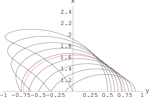
Figure 2: Parametric plot of the solutions $(x(\sigma),y(\sigma))$ with initial conditions $x(0)=1$, $y^{\prime}(0)=0$, and fixed $y(0)$ in the range $0.5<y(0)<0.9.$

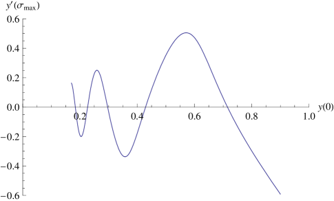
Figure 3: $y^{\prime}(\sigma_{max})$ for the solution of equation of motion as a function of the initial condition $y(0).$

To be more systematic, one can plot $y^{\prime}(\sigma_{max})$ for the solutions of the equation of motion as a function of the initial condition $y(0)$. This is illustrated for the range of $0.175<y(0)<0.9$ in figure 3. We stopped at $y(0)\approx 0.2$ since numerical load becomes heavier for smaller value of $y(0)$. The zero of this function near $y(0)\approx 0.715$ is readily apparent. Also apparent are other zeros at $y(0)$ taking approximate values 0.184, 0.227, 0.297, 0.429. The significance of these other zeros and the behavior for smaller values of $y(0)$ will be discussed in the appendix A.

It would be instructive to explore how these solutions change as the values of $w$ is varied keeping $x_{b}$ fixed. This is illustrated in figure 4 where we have chosen to plot $U/U_{b}$ instead of $x$ as a function of $y$ to facilitate the comparison with configurations described in [1, 2]. The curves with larger values of $y$ corresponds to smaller values of $w$. From figure 4, it is apparent that most of the energy comes from the rest masses of W and anti-W when they are separated by large distances with small values of $w$.

Figure 4: Solution of equation of motion and the boundary condition for D3-branes placed at $U=U_{b}$, illustrated as $U/U_{b}$ as a function of $y$ for various values of $w$. The configuration with large $y$ corresponds to small $w$ and large $S$.

A very useful exercise is to plot $E$ as a function of $S$ by substituting the solution to (6) and (7). The result of this analysis is illustrated in figure 5. For small values of $S$, we find

$$E\sim\sqrt{\frac{\pi TS}{2}}$$ (25)

which has the form of the relation (8) for rotating rigid string in flat space, with the effective tension $T={U_{b}^{2}/2\pi\lambda^{1/2}}$ for strings extended along $U=U_{b}$. For large $S$, the energy asymptotes to twice the rest mass of the W-bosons. There is a factor of $\sqrt{2}$ difference between (8) since the open strings are not folded. (This gives rise to factors of 1/2 in $E$ and $S$.)

Figure 5: Plot of energy $E$ v.s. angular momentum $S$ for a positronium-like bound state of W/anti-W pair in a strongly coupled ${\cal N}=4$ theory with gauge group $SU(N)\times U(1)$.

These semi-classical steady state rotating open string solutions in $AdS_{5}\times S_{5}$ provide the main tool for the subsequent analysis in the remainder of this paper. They are positronium-like bound state of W and an anti-W. In stating such a result, one should keep in mind that the semi-classical analysis of the type presented here is subject to world sheet ($\alpha^{\prime}$) and space-time ($g_{s}$) quantum corrections. Indeed, rigid rotating strings typically decay via fragmentation and emission of closed strings [11, 12, 13, 14, 15]. Fortunately, as was the case for [9], the strong ’t Hooft coupling and large $N$ limit allows one to treat the semi-classical analysis to be reliable quantitatively, in that the quantum corrections are small.

The fact that there are positronium-like bound states in the spectrum of $SU(N+1)\rightarrow SU(N)\times U(1)$ theory implies that they should appear as resonances, for example, in $2\rightarrow 2$ scattering process. Recently, there have been significant efforts directed toward computations of scattering amplitudes taking advantage of the unique features of ${\cal N}=4$ supersymmetry. See e.g. [16, 17, 18] for reviews and references to recent developments. Perhaps some of these techniques can be used to confirm the rich spectrum of ${\cal N}=4$ theory in the Coulomb branch.

The rigid rotating strings in the treatment of [9] were steady state solution with respect to global time of $AdS_{5}\times S_{5}$. This allowed their mass to be compared to the scaling dimension of gauge invariant operators. The fact that the positronium- like state found in this note is a steady state with respect to Poincare time makes similar interpretation somewhat subtle. One way to overcome this obstacle might be to consider open strings ending on giant gravitons blown up in the $AdS_{5}$ [19, 20], along the lines of [21, 22, 23]. Open spinning strings in $AdS_{5}\times S_{5}$ and related models were also considered in [24, 25, 26, 27].

In the following section, we examine how the analysis of the present section is modified when the non-commutativity parameter is non-vanishing.

3 Positronium in non-commutative SYM

The supergravity background corresponding to non-commutative Yang-Mills theory has a relatively simple form [3, 4, 5] whose metric and the NSNS 2-form are given by

$$ds^{2} = \alpha^{\prime}\left({U^{2}\over\sqrt{\lambda}}\left(-dt^{2}+dx_{1}^{2}+{1\over 1+\lambda^{-1}\Delta^{4}U^{4}}(dr^{2}+r^{2}d\phi^{2})\right)+{\sqrt{\lambda}\over U^{2}}(dU^{2}+U^{2}d\Omega_{5}^{2}\right)$$ (26)

$$B = \alpha^{\prime}{\Delta^{2}U^{4}\over\lambda+\Delta^{4}U^{4}}rdr\wedge d\phi\ .$$ (27)

As we reviewed in the introduction, the status of Wilson loop observables along the lines of [1, 2] remains unclear, in light of the fact that the world sheet configuration $r(U)$ with finite $U_{min}$ does not take finite value when $U\rightarrow\infty$ [4, 5]. Regarding this issue, it is worth noting an interesting observation made in [6] that $r(U=\infty)$ can be made to take on finite value if the strings were made to move at a special fixed velocity, depending on the distance separating the endpoints of the strings at $U=\infty$, along the non-commutative plane. The physical significance of the velocity required for the $q\bar{q}$-pair is not immediately obvious. The study of positronium-like bound states of W and anti-W would, therefore, provides an interesting new perspective on the nature of interactions between opposite charges in non-commutative field theories. Our analysis of the positronium-like bound state will suggest a natural interpretation for the velocity of the moving strings used in [6] which we will elaborate in section 4.

Let us begin by considering a steady state rotating ansatz for the strings. The action for the world sheet will then take the form

$$L = \int d\tau\,d\sigma\,{U(\sigma)^{2}\over\sqrt{\lambda}}\sqrt{\left(1-{\omega^{2}r(\sigma)^{2}\over 1+\lambda^{-1}\Delta^{4}U(\sigma)^{4}}\right)\left({r^{\prime}(\sigma)^{2}\over 1+\lambda^{-1}\Delta^{4}U(\sigma)^{4}}+{\lambda U^{\prime}(\sigma)^{2}\over U(\sigma)^{4}}\right)}$$ (29)

$$\qquad+{\omega\Delta^{2}r(\sigma)r^{\prime}(\sigma)U(\sigma)^{4}\over\lambda+\Delta^{4}U(\sigma)^{4}}\ .$$

Just as we did before, it is useful to rescale

$$U(\sigma)={\lambda^{1/2}U_{0}\over x(\sigma)},\qquad r(\sigma)={1\over U_{0}}y(\sigma),\qquad\omega=U_{0}w,\qquad\Delta={\lambda^{-1/4}\over U_{0}}q$$ (30)

and introduce a Lagrange multiplier $e$ so that the action becomes

$$L={f\over 2}(e+{1\over e}\left(\left(1+{q^{4}\over x(\sigma)^{4}}\right)x^{\prime}(\sigma)^{2}+y^{\prime}(\sigma)^{2}\right)+{q^{2}wy(\sigma)y^{\prime}(\sigma)\over q^{4}+x(\sigma)^{4}}$$ (31)

where

$$f^{2}={q^{4}+x(\sigma)^{4}(1-w^{2}y(\sigma)^{2})\over(q^{4}+x(\sigma)^{4})^{2}}\ .$$ (32)

With the gauge condition

$$e=f$$ (33)

the action will take the form

$$L={1\over 2}\left(\left(1+{q^{4}\over x(\sigma)^{4}}\right)x^{\prime}(\sigma)^{2}+y^{\prime}(\sigma)^{2}\right)-V\left(x(\sigma),y(\sigma)\rule{0.0pt}{8.61108pt}\right)+A_{y}\left(x(\sigma),y(\sigma)\rule{0.0pt}{8.61108pt}\right)y^{\prime}(\sigma)$$ (34)

$$V\left(x(\sigma),y(\sigma)\rule{0.0pt}{8.61108pt}\right)=-{f^{2}\over 2},\qquad A_{y}\left(x(\sigma),y(\sigma)\rule{0.0pt}{8.61108pt}\right)={q^{2}wy(\sigma)\over q^{4}+x(\sigma)^{4}}\ ,$$ (35)

with a constraint

$$H={1\over 2}\left(\left(1+{q^{4}\over x(\sigma)^{4}}\right)x^{\prime}(\sigma)^{2}+y^{\prime}(\sigma)^{2}\right)-{1\over 2}f^{2}=0\ .$$ (36)

In order to make this action look more like a motion of a particle in a potential, one can further change variables

$$z(x)=1+\int_{1}^{x}dx_{0}\left(1+{q^{4}\over x_{0}(\sigma)^{4}}\right)^{1/2}$$ (37)

so that the action is

$$L={1\over 2}\left(z^{\prime}(\sigma)^{2}+y^{\prime}(\sigma)^{2}\right)-V\left(z(\sigma),y(\sigma)\rule{0.0pt}{8.61108pt}\right)+A_{y}\left(z(\sigma),y(\sigma)\rule{0.0pt}{8.61108pt}\right)y^{\prime}(\sigma)\ .$$ (38)

Note that $z=0$ does not have any special significance. The boundary points $x=0$ are mapped to $z=-\infty$. This action describes a point particle moving in a $(z,y)$ plane with potential $V(z,y)$ in the presence of a magnetic field given by a vector potential $A_{y}(z,y)$. Unlike in the case of the constant magnetic field, the $A_{y}$ term, which came from the NSNS $B$-field, does affect the equation of motion. It also changes the relation between $z^{\prime}(\sigma)$ and its conjugate momentum. However, it does not affect the conservation of the Hamiltonian

$$H={1\over 2}\left(z^{\prime}(\sigma)^{2}+y^{\prime}(\sigma)^{2}\right)+V\left(z(\sigma),y(\sigma)\rule{0.0pt}{8.61108pt}\right)\ .$$ (39)

For the purpose of solving the equations of motion numerically, the $(x,y)$ coordinates suffice. The boundary condition for the $y(\sigma)$ for this case is

$$y^{\prime}(\sigma)+{q^{2}wy(\sigma)\over q^{4}+x(\sigma)^{4}}=0\ .$$ (40)

For the purpose of illustration, let us consider setting $w=0.05$, $x_{b}=1$, and $q$ ranging from $q=0$ to $q=5.5$. The solutions corresponding to this case is illustrated in figure 6.

Figure 6: Positronium-like bound state of W/anti-W pair in dual supergravity description of non-commutative supersymmetric Yang-Mills theory. Here, we have taken $0\leq q\leq 5.5$ and $\omega=0.05.$

One notable feature of the solutions illustrated in figure 6 is the fact that the position of the string end points $y(0)$ and $y(\sigma_{max})$, as well as the maximum $x_{max}$, appears to be unaffected by changes in $q$. This may well be an artifact of probing only narrow range of parameters. Nonetheless, the independence of these data on $q$ seems remarkably robust and is suggestive that there might be some hidden symmetry, although we were unable to identify one.

Note that as the non-commutativity is increased, the boundary condition will tilt the string as it ends on the brane, causing a narrow fluxtube to appear before the strings penetrate the bulk AdS region, indicating the spreading of the flux. This is compatible with the intuition that the positions of the quarks are becoming more uncertain as $q$ is increased [4, 5]. Nonetheless, the existence of these solutions indicates that a W/anti-W bound state do exist. One can further study the relation between energy and spin along the lines of what we illustrated in figure 5. We have repeated this analysis of determining $E$ as a function of $S$ for various fixed values of $q=0.5$, $q=1$ and $q=5$. Rather remarkably, we found that the relation $E(S)$ is unaffected by the changes in $q$. This may also be an indication that there is some hidden symmetry which we have not yet accounted.

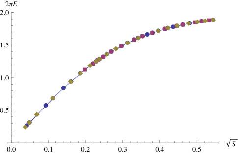
Figure 7: Numerical computation of $E(S)$ for $q=0.5$, $q=1.0$ and $q=5.0$ superposed on the $q=0$ curve.

It should be noted that this analysis closely parallels that of [28] which also considered the dynamics of rotating open strings ending on a D7-brane. In fact the equation of motion and the solution we present are identical. Yet, we reach a drastically different conclusion, namely that $E(S)$, illustrated in figure 7, is insensitive to the effects of non-commutative deformation. The cause of this apparent discrepancy is the fact that the angular momentum computed in [28] did not include the contribution from the Kalb-Ramond term of the world sheet action. Kalb-Ramond terms certainly contribute to the canonical momentum and angular momentum for the dynamics of open strings [29]; and with the contribution from the Kalb-Ramond included, we find compelling numerical indication that $E(S)$ is independent of the non-commutativity deformation. This is an important conclusion since it implies, in spite of the puzzling behavior of the Wilson lines [4, 5], that the quark anti-quark potential is unaffected by the non-commutative parameter.

4 Canonical momentum of the moving $q\bar{q}$ pair

In the analysis of the positronium-like bound state, we found that the relation between the energy $E$ and the canonical angular momentum $S$ which includes the contribution of the Kalb-Ramond term is unaffected by the changes in the non-commutativity parameter. This observation offers a natural interpretation for the specific velocity of the moving $q\bar{q}$ pair in the analysis of [6].

Let us begin by recalling the construction of [6]. A string world sheet embedded in the supergravity background (26) which we re-express in Cartesian coordinates [3, 4, 5]

$$ds^{2} = \alpha^{\prime}\left\{{U^{2}\over\sqrt{\lambda}}(-dt^{2}+dx_{1}^{2})+{\sqrt{\lambda}U^{2}\over\lambda+U^{4}\Delta^{4}}(dx_{2}^{2}+dx_{3}^{2})+{\sqrt{\lambda}\over U^{2}}dU^{2}+\sqrt{\lambda}d\Omega_{5}^{2}\right\}$$ (41)

$$B_{23} = {\alpha^{\prime}\Delta^{2}U^{4}\over\lambda+\Delta^{4}U^{4}},$$ (42)

will minimize the action

$$S=\int dt\,dU\sqrt{-g_{00}\left(g_{UU}+g_{33}\left({dx_{3}(U)\over dU}\right)^{2}\right)}$$ (43)

where we have taken the $q\bar{q}$ pair to be separated along the $x_{3}$ direction and stationary in the $x_{1},x_{2}$ directions. If the $q\bar{q}$ pair moves in the $x_{2}$ direction with velocity $v$, the action (43) is modified to take the form

$$S=\int dt\,dU\sqrt{-(g_{00}+g_{22}v^{2})\left(g_{UU}+g_{33}\left({dx_{3}(U)\over dU}\right)^{2}\right)}-B_{23}v{dx_{3}(U)\over dU}.$$ (44)

As was the case in [1, 2], it is possible to constrain

$${\delta S\over\delta x_{3}^{\prime}(U)}=\mbox{fixed}$$ (45)

which can be solved for $x_{3}^{\prime}(U)$

$$x_{3}^{\prime}(U)=c(v,U_{min})+{\cal O}(U^{-4})$$ (46)

giving rise to the linearly growing $x_{3}(U)$ with the slope $c(v,U_{min})$ depending on $v$ and $U_{min}$ illustrated in figure 1.

The key observation in [6] is the fact that by choosing $v$ to take a specific value

$$v=-{\Delta^{2}U_{min}^{2}\over\sqrt{\lambda}}$$ (47)

the slope constant $c(v,U_{min})$ vanishes and the asymptotic behavior of $x_{3}^{\prime}(U)$ simplifies drastically to take the form

$$x_{3}^{\prime}(U)={\sqrt{\lambda}U_{min}^{2}\over U^{2}\sqrt{U^{4}-U_{min}^{4}}}.$$ (48)

This, in fact, is identical to the configuration of [1, 2] at zero velocity and vanishing non-commutativity.

There is a natural interpretation of the special velocity (47) in light of the conclusion of the previous section. If one considers the canonical momentum, one finds that it vanishes identically, precisely when $v$ takes the value (47).

$$P_{2} = \left.\int dU{d\over dv}\left(\sqrt{-(g_{00}+g_{22}v^{2})\left(g_{UU}+g_{33}\left({dx_{3}(U)\over dU}\right)^{2}\right)}-B_{23}v{dx_{3}(U)\over dU}\right)\right|_{v=-\Delta^{2}U_{min}^{2}/\sqrt{\lambda}}$$ (49)

$$= \int dU\,{\Delta^{2}\sqrt{\lambda}U^{2}U_{min}^{2}\over\lambda+\Delta^{4}U^{4}}\left({1\over\sqrt{U^{4}-U_{min}^{4}}}-{1\over\sqrt{U^{4}-U_{min}^{4}}}\right)$$ (50)

$$= 0$$ (51)

This clarifies the physical significance of the special value (47) for $v$. The quark anti-quark potential are well defined in non-commutative plane if one fixes the momentum, instead of the position, of the quarks in the direction orthogonal to the direction separating the quarks. In order to fix the value of this momentum to zero, one sets $v$ to the special value (47). For that value of $v$, the quark anti-quark potential has a smooth commutative limit. In fact, the potential is insensitive to the non-commutativity parameter. This observation further emphasizes the importance of considering the canonical momentum including the contribution of the Kalb-Ramond term.

5 Conclusions

In this article, we considered the dynamics of W-boson and anti-W-boson pair in ${\cal N}=4$ supersymmetric non-commutaitive Yang-Mills theory in 3+1 dimensions, with spontaneously broken gauge group $SU(N+1)\rightarrow SU(N)\times U(1)$. We studied this system at large $N$ and large ’t Hooft coupling, where the dual supergravity description in terms of a probe D3-brane embedded into an $AdS_{5}\times S_{5}$ background in type IIB string theory is valid. In this description, the W-bosons are represented as strings stretching from the D3-brane to the horizon of $AdS_{5}$.

The question of how to correctly formulate quark anti-quark potential as a holographic observable, along the lines of [1, 2] for the supergravity dual of non-commutative field theory, has been a long standing puzzle [4, 5]. It is, therefore, quite interesting that positronium-like bound states of W/anti-W pair can be shown to exist in non-commutative field theories at large $N$ and large ’t Hooft coupling, and for their energy and spin to be completely insensitive to the non-commutativity parameter, as we illustrated in figure 7. In order to arrive at this conclusion, it is important to consider the canonical angular momentum including the contribution of the Kalb-Ramond term. Viewing $q\bar{q}$ potential as being at fixed momentum, as opposed to fixed position in the direction transverse to the direction separating the quarks, also gives rise to a simple result independent of the non-commutativity parameter. By using the mixed position space/momentum space quantum numbers as a label, the holographic interpretation of the Wilson loop observables in non-commutative gauge theories appears to clarify significantly.

Appendix A Excited positronium-like bound states

One obvious issue which we did not explore fully in section 2 is the meaning of other roots at $y(0)$ taking values 0.184, 0.227, 0.297, and 0.429 in figure 3. It is straight forward to illustrate the trajectory $(x(\sigma),y(\sigma))$ associated with these solutions. They are illustrated in figure 8. Each of these solutions respects the boundary condition at both endpoints of the string world sheet. As such, they also correspond to positronium-like W/anti-W bound states of the theory which are effectively stable in the large $N$, large $\lambda$ limit. For the cases illustrated in figure 8.a and 8.c, corresponding to $y(0)=0.429$ and $y(0)=0.227$, respectively, the string hits $y(\sigma)=1$ where the piece of the string is moving at the speed of light in $AdS_{5}$. At that point, one expects the string to fold and return to the brane along the same path it took to get there. For the cases illustrated in figure 8.b and 8.d, the string self-intersects an integer number of times before returning to the brane. While it is natural to expect a state like this to decay in an interacting theory, this effect is suppressed at leading order in the $1/N$ expansion. Identical set of configurations were first found for the open strings ending on D7-branes in [10]

(a)	(b)
(c)	(d)

Figure 8: Solutions to the equation of motion $(x(\sigma),y(\sigma))$ with initial conditions (a) $y(0)=0.429$, (b) $y(0)=0.297$, (c) $y(0)=0.227$, (d) $y(0)=0.184$.

There is no reason not to expect this pattern of increasingly self-intersecting states to exist as $y(0)$ approaches zero, although they are harder to discover using a numerical algorithm simply because the proper time of trajectory, parametrized by $\sigma$, becomes large. After all, they are precisely analogous to a different way of shooting a pin-ball through the potential (17), such that it crosses the $y=0$ axis as it rolls in the $x\gg 1$ region where there is a shallow oscillating potential along the $y$ direction. The fact that there is this rich spectrum of excited positronium-like bound states is a prediction of ${\cal N}=4$ SYM at large $N$ and large $\lambda$. Similar richness in the allowed string configurations was noted also in [30] where quark anti-quark potential for ${\cal N}=4$ SYM in Coulomb branch was studied using the techniques of AdS/CFT correspondence.

Appendix B Positronium in Magnetic Field

Another simple extension of the analysis of section 2 is turning on a uniform magnetic field in the plane of rotation of the positronium. This issue was originally investigated in the context of open strings ending on D7-branes in [31]. We will repeat the analysis here because it is a useful warm-up exercise before addressing the non-commutative case.

Let us begin by reviewing the semi-classical trajectory of the charges forming a bound state in a magnetic field.

A single moving charge in a magnetic field follows the standard circular orbit. If they are two opposite charges, they can orbit around a common axis with the same angular velocity $\omega$, and radius $r_{1}$ and $r_{2}$ as illustrated in figure 9.

Figure 9: Circular orbit of charged particle anti-particle pair in a magnetic field.

The equation of motion for the two charges are

$$m\omega^{2}r_{1}={q^{2}\over(r_{1}+r_{2})^{2}}+qB\omega r_{1}$$ (52)

$$m\omega^{2}r_{2}={q^{2}\over(r_{1}+r_{2})^{2}}-qB\omega r_{2}$$ (53)

from which we infer

$$m\omega^{2}R={2q^{2}\over R^{2}},\qquad m\omega^{2}(r_{1}-r_{2})=q\omega RB,\qquad R=(r_{1}+r_{2})\ .$$ (54)

So we see that for fixed $\omega$ the effect of non-vanishing $B$ field is to shift the axis of rotation away from the center of mass without affecting the dipole length $R$.

Let us examine how the magnetic field affects the large $N$ large $\lambda$ description in terms of semi-classical strings in $AdS_{5}\times S_{5}$. The only change in the dual type IIB picture is that there will be a constant NSNS 2-form potential along the plane of rotation of the string. This will affect (10) by adding a term

$$L_{B}=\int d\tau\,d\sigma\,\omega Br(\sigma)r^{\prime}(\sigma)\ .$$ (55)

After the same change of variables as in the previous section, as well as scaling

$$B={\sqrt{\lambda}U_{0}^{2}b\over 2\pi}$$ (56)

this term becomes

$$L_{B}={\lambda^{1/2}\over 2\pi}\int d\tau\,d\sigma\,bwy(\sigma)y^{\prime}(\sigma)\ .$$ (57)

Note that this term is a total derivative, and does not affect the equation of motion. It does, however, modify the Neumann boundary condition, when combined with (13), to read

$$y^{\prime}(\sigma)=-bwy(\sigma)$$ (58)

at the boundaries of the open string world sheet $\sigma=0$ and $\sigma=\sigma_{max}$. This boundary condition, combined with the conservation of the Hamiltonian, also implies

$$x^{\prime}(\sigma)=\pm\sqrt{{1-w^{2}(1+b^{2}x(\sigma)^{4})y(\sigma)^{2}\over x(\sigma)^{4}}}$$ (59)

at the endpoints of the open string. We are, therefore, faced with a similar problem of scanning over the set of initial condition parametrized by $y(0)$ so that the boundary condition at $\sigma=\sigma_{max}$ is satisfied. The only difference between this and the analysis of the previous two sections is the change in the boundary condition (58).

For the sake of concreteness, we picked $x_{b}=1$, $w=1$, and scanned $b$ in the range $0<b<10$. The result of this analysis is illustrated in figure 10.

Figure 10: Configuration of spinning open string ending on a D3-brane at fixed $U_{b}$ in $AdS_{5}\times S_{5}$ with non-vanishing $B_{23}$. Here, we consider $0\leq b\leq 10$ with $\omega=1.$

Unlike what we found in the semi-classical analysis of the positronium in a magnetic field, the length of the dipole does appear to shrink as $b$ is increased. This is partly necessitated by the requirement that (59) is real. It is also interesting to note that the two endpoints are located roughly symmetrically around the axis of rotation. It is also interesting to note that as $B$ is increased, the string appear to be approaching a configuration with a fold.

There is one more curious feature concerning the shape of the strings illustrated in figure 10. As $b$ is varied keeping $\omega$ fixed, the maximum value of $x_{max}\approx 1.64$ of the trajectory appears roughly constant. Closer examination shows, $x_{max}$ does vary mildly as $b$ is varied. We will encounter similar behavior for the semi-classical open string configurations in the non-commutative theory.

References

- [1] S.-J. Rey and J.-T. Yee, “Macroscopic strings as heavy quarks in large gauge theory and anti-de Sitter supergravity,” Eur. Phys. J. C22 (2001) 379–394, hep-th/9803001.
- [2] J. M. Maldacena, “Wilson loops in large field theories,” Phys. Rev. Lett. 80 (1998) 4859–4862, hep-th/9803002.
- [3] A. Hashimoto and N. Itzhaki, “Non-commutative Yang-Mills and the AdS/CFT correspondence,” Phys. Lett. B465 (1999) 142–147, hep-th/9907166.
- [4] A. Hashimoto, “Holography and Non-commutative Geometry,” Proceedings of Summer Institute ’99, http://www-hep.phys.s.u-tokyo.ac.jp/proceeding/si99/1st_week/hashimoto.ps.gz.
- [5] J. M. Maldacena and J. G. Russo, “Large limit of non-commutative gauge theories,” JHEP 09 (1999) 025, hep-th/9908134.
- [6] M. Alishahiha, Y. Oz, and M. M. Sheikh-Jabbari, “Supergravity and large noncommutative field theories,” JHEP 11 (1999) 007, hep-th/9909215.
- [7] S. R. Das and S.-J. Rey, “Open Wilson lines in noncommutative gauge theory and tomography of holographic dual supergravity,” Nucl. Phys. B590 (2000) 453–470, hep-th/0008042.
- [8] D. J. Gross, A. Hashimoto, and N. Itzhaki, “Observables of non-commutative gauge theories,” Adv. Theor. Math. Phys. 4 (2000) 893–928, hep-th/0008075.
- [9] S. S. Gubser, I. R. Klebanov, and A. M. Polyakov, “A semi-classical limit of the gauge/string correspondence,” Nucl. Phys. B636 (2002) 99–114, hep-th/0204051.
- [10] M. Kruczenski, D. Mateos, R. C. Myers, and D. J. Winters, “Meson spectroscopy in AdS/CFT with flavour,” JHEP 07 (2003) 049, hep-th/0304032.
- [11] D. Mitchell, N. Turok, R. Wilkinson, and P. Jetzer, “The decay of highly excited open strings,” Nucl. Phys. B315 (1989) 1.
- [12] R. B. Wilkinson, N. Turok, and D. Mitchell, “The decay of highly excited closed strings,” Nucl. Phys. B332 (1990) 131.
- [13] D. Mitchell, B. Sundborg, and N. Turok, “Decays of massive open strings,” Nucl. Phys. B335 (1990) 621.
- [14] H. Okada and A. Tsuchiya, “The decay rate of the massive modes in type I superstring,” Phys. Lett. B232 (1989) 91.
- [15] V. Balasubramanian and I. R. Klebanov, “Some aspects of massive world-brane dynamics,” Mod. Phys. Lett. A11 (1996) 2271–2284, hep-th/9605174.
- [16] L. J. Dixon, “Calculating scattering amplitudes efficiently,” hep-ph/9601359.
- [17] F. Cachazo and P. Svrcek, “Lectures on twistor strings and perturbative Yang-Mills theory,” hep-th/0504194.
- [18] L. J. Dixon, “Gluon scattering in super-Yang-Mills theory from weak to strong coupling,” 0803.2475.
- [19] M. T. Grisaru, R. C. Myers, and O. Tafjord, “SUSY and Goliath,” JHEP 08 (2000) 040, hep-th/0008015.
- [20] A. Hashimoto, S. Hirano, and N. Itzhaki, “Large branes in AdS and their field theory dual,” JHEP 08 (2000) 051, hep-th/0008016.
- [21] D. Berenstein and S. E. Vazquez, “Integrable open spin chains from giant gravitons,” JHEP 06 (2005) 059, hep-th/0501078.
- [22] D. Berenstein, D. H. Correa, and S. E. Vazquez, “Quantizing open spin chains with variable length: An example from giant gravitons,” Phys. Rev. Lett. 95 (2005) 191601, hep-th/0502172.
- [23] D. Berenstein, D. H. Correa, and S. E. Vazquez, “A study of open strings ending on giant gravitons, spin chains and integrability,” JHEP 09 (2006) 065, hep-th/0604123.
- [24] F. Bigazzi, A. L. Cotrone, L. Martucci, and L. A. Pando Zayas, “Wilson loop, Regge trajectory and hadron masses in a Yang- Mills theory from semiclassical strings,” Phys. Rev. D71 (2005) 066002, hep-th/0409205.
- [25] M. Kruczenski, L. A. P. Zayas, J. Sonnenschein, and D. Vaman, “Regge trajectories for mesons in the holographic dual of large- QCD,” JHEP 06 (2005) 046, hep-th/0410035.
- [26] K. Okamura, Y. Takayama, and K. Yoshida, “Open spinning strings and AdS/dCFT duality,” JHEP 01 (2006) 112, hep-th/0511139.
- [27] N. Mann and S. E. Vazquez, “Classical open string integrability,” JHEP 04 (2007) 065, hep-th/0612038.
- [28] D. Arean, A. Paredes, and A. V. Ramallo, “Adding flavor to the gravity dual of non-commutative gauge theories,” JHEP 08 (2005) 017, hep-th/0505181.
- [29] D. Bigatti and L. Susskind, “Magnetic fields, branes and noncommutative geometry,” Phys. Rev. D62 (2000) 066004, hep-th/9908056.
- [30] J. A. Minahan and N. P. Warner, “Quark potentials in the Higgs phase of large supersymmetric Yang-Mills theories,” JHEP 06 (1998) 005, hep-th/9805104.
- [31] K. D. Jensen, A. Karch, and J. Price, “Strongly bound mesons at finite temperature and in magnetic fields from AdS/CFT,” JHEP 04 (2008) 058, 0801.2401.