Stability of an $[N/2]$-dimensional invariant torus in the Kuramoto model at small coupling

Abstract

When the natural frequencies are allocated symmetrically in the Kuramoto model there exists an invariant torus of dimension $[N/2]+1$ ($N$ is the population size). A global phase shift invariance allows to reduce the model to $N-1$ dimensions using the phase differences, and doing so the invariant torus becomes $[N/2]$-dimensional. By means of perturbative calculations based on the renormalization group technique, we show that this torus is asymptotically stable at small coupling if $N$ is odd. If $N$ is even the torus can be stable or unstable depending on the natural frequencies, and both possibilities persist in the small coupling limit.

1 Introduction

The Kuramoto model [1, 2, 3] has become the basic framework for the description of macroscopic synchronization; a phenomenon observed in a variety of natural and artificial systems [4, 5]. Kuramoto [1] considered a population of all-to-all weakly coupled oscillators such that their interaction could be reduced to their phases:

$$\dot{\theta}_{j}=\omega_{j}+\frac{\varepsilon}{N}\sum_{l=1}^{N}f(\theta_{l}-\theta_{j}),\quad j=1,2,\cdots,N,$$ (1)

where $\theta_{j}$ and $\omega_{j}$ are, respectively, the phase and the natural frequency of the $j$-th oscillator, and $\varepsilon$ is the coupling strength. Kuramoto adopted a sinusoidal coupling function $f(\cdot)=\sin(\cdot)$ together with a symmetric frequency distribution of the natural frequencies, what resulted very useful for the theoretical analysis of the model.

Originally, it was useful and instructive to consider the thermodynamic limit of (1), $N\to\infty$. Finite-size effects have remained unsolved for a long time and only recently significative advances have been achieved [6, 7, 8, 9, 10]. Also some attention has been recently devoted to the small-$N$ behavior of the Kuramoto model by Maistrenko and coworkers from the point of view of dynamical systems theory [11, 12, 13].

In this paper we study the Kuramoto model with a finite population, and with the natural frequencies allocated symmetrically around the mean frequency. One of the reasons that motivates this problem is the fact that most works on the Kuramoto model have assumed that the natural frequencies are distributed according to a symmetric probability density, and as a consequence it is usual that numerical simulations are carried out selecting frequencies not at random, but reflecting the inherent symmetry of the frequency distribution. In particular, several works [11, 12, 13, 14] have recently investigated phase diagrams of the Kuramoto model with a finite population $N$ under the assumption that the natural frequencies are allocated symmetrically. It has been shown that under these assumptions, finite $N$ and symmetry of the natural frequencies, model (1) exhibits a peculiar type of chaos dubbed ‘phase chaos’.

Of more importance for this work is the finding in [14] that the phase space contains an $[N/2]$-dimensional invariant torus. This torus has been thought to be unstable (i.e. repelling) when $\varepsilon\to 0$ [12, 13, 14]. This belief is probably motivated by the difficulty of investigating numerically the phase diagram for small $\varepsilon$ due to the extremely weak (in)stability of invariant sets in that limit. One of the purposes of this paper is to reveal the phase diagrams of the Kuramoto model at small coupling and different values of $N$. Our analytical results are obtained by using the renormalization group (RG) method, which is one of the singular perturbation methods. Our results firmly establish the stability of the mentioned invariant torus on rigorous mathematical grounds. In particular, we give general results for any finite $N$, and some small populations ($N=3,..,7$) are investigated in more detail.

2 Basic definitions

Due to the mean-field character of the Kuramoto model we may arbitrarily label the natural frequencies from the smaller to the larger: $\omega_{1}\leq\omega_{2}\leq\cdots\leq\omega_{N}$. Moreover, by going into a suitable rotating framework we set the mean frequency equal to zero without loss of generality. For the discussion to follow it is worth to note that if there are not coincident natural frequencies (i.e. $\omega_{1}<\omega_{2}<\cdots<\omega_{N}$), some degree of synchronization, $\left<\dot{\theta}_{i}\right>=\left<\dot{\theta}_{j}\right>$ for some (or all) $i\neq j$, is only achieved for a coupling strength larger than some positive constant $\varepsilon_{c}$.

Next, we rewrite the Kuramoto model for the convenience of our analysis. Due to the invariance of the global quantity $\Theta=\sum_{l=1}^{N}\theta_{l}$, the Kuramoto model can be reduced in one dimension by changing to a new set of coordinates: $\varphi_{j}=\theta_{j+1}-\theta_{j},\,j=1,\cdots,N-1$. It is also useful to define “frequency gaps” $\Delta_{j}=\omega_{j+1}-\omega_{j},\,j=1,\cdots,N-1$. In the new variables the Kuramoto model has this structure

$$\dot{\varphi}_{j}=\Delta_{j}+\varepsilon\,\Xi_{j}(\varphi_{1},\varphi_{2},\ldots,\varphi_{N-1}),\quad j=1,\cdots,N-1.$$ (2)

Maistrenko and coworkers [12, 13, 14] found that if the natural frequencies are symmetrically selected ($\omega_{i}=-\omega_{N-i+1}$ $\Rightarrow$ $\Delta_{j}=\Delta_{N-j}$) the Kuramoto model has an invariant manifold $\mathcal{M}$, namely a torus of dimension $[N/2]$, which is given by $\mathcal{M}=\{\varphi_{i}=\varphi_{N-i}\}$. (In the original coordinates, $\mathcal{M}$ is any of the tori that —parameterized by the invariant $\Theta$— foliate an $([N/2]+1)$-dimensional torus; thus if one selects $\Theta=0$, $\mathcal{M}=\{\theta_{i}=-\theta_{N-i+1}\}$.)

3 Main results

In Refs. [12, 13, 14] it was shown that for some values of the parameters $\omega_{i}$ and $\varepsilon$, the dynamics approaches the invariant torus $\mathcal{M}$ or an attractor $\mathcal{A}\subset\mathcal{M}$. They reported that the regions of parameters with stable $\mathcal{M}$ or $\mathcal{A}$ are close to, or inside, synchronization regions (what implies that $\varepsilon$ is larger than some positive number if $\omega_{i}\neq\omega_{j\neq i}$). Thus, there is a common belief that far from synchronization, as the coupling strength goes to zero ($\varepsilon\to 0$), the dynamics fills the whole phase space, the $N-1$ dimensional torus $\{\varphi_{j}\}$. So far, many numerical results confirmed this expectation [12, 13, 14]. However, we show in this paper that this is not true. We have found that in the limit $\varepsilon\to 0$:

1. If $N$ is odd the $(N-1)/2$-dimensional invariant torus $\mathcal{M}$ is, unless there are special resonant conditions among the natural frequencies, asymptotically stable.

2. If $N$ is even the $N/2$-dimensional invariant torus $\mathcal{M}$ can be stable or unstable depending on the particular disposition of the natural frequencies.

Statements (i) and (ii) are consequence of three Theorems to be proved by using the RG method, which is a powerful singular perturbation method for differential equations proposed in [15, 16]. Recently, mathematical foundation of the RG method was given in [17, 18] showing that the RG method is useful as well to investigate existence and stability of invariant manifolds. We present a brief review of the RG method in Section 7.1, and the proofs of the main theorems in this paper are shown in Section 7.2 and 7.3.

4 Odd $N$

In this section, we investigate the stability of the invariant torus $\mathcal{M}$ for odd $N$. For two particular cases, $N=3$ and $5$, the phase diagrams are completely uncovered.

One of the main theorems in this paper is as follows:

Theorem 1.     Suppose that $N=2M-1$ is an odd number. If the natural frequencies satisfy the following nonresonance condition:

$$\left\{\begin{array}[]{l}\omega_{i}=\omega_{j}\,\,\,\mathrm{if\,and\,only\,if}\,\,\,i=j,\\ \omega_{k}+\omega_{j}=2\omega_{i}\,\,\,\mathrm{if\,and\,only\,if}\,\,\,i=k=j\,\,\mathrm{or}\,\,j=2M-k,i=M,\\ \omega_{i}+\omega_{j}=\omega_{k}+\omega_{l}\,\,\,\mathrm{if\,and\,only\,if}\,\,\,i=j=k=l\,\,\mathrm{or}\,\,j=2M-i,l=2M-k,\\ 3\omega_{i}=\omega_{j}+\omega_{k}+\omega_{l}\,\,\,\mathrm{if\,and\,only\,if}\,\,\,i=j=k=l,\\ \omega_{i}+2\omega_{k}=\omega_{j}+2\omega_{l}\,\,\,\mathrm{if\,and\,only\,if}\,\,\,i=j,k=l\,\,\mathrm{or}\,\,j=2M-i,k=M,l=i,\end{array}\right.$$ (8)

then there exists a positive constant $\varepsilon_{0}$, which depends on the natural frequencies, such that if $0<\varepsilon<\varepsilon_{0}$, the invariant torus $\mathcal{M}$ is asymptotically stable and the transverse Lyapunov exponents of $\mathcal{M}$ are of $O(\varepsilon^{3})$.

Equation (8) can be rewritten as a condition for $\Delta_{j}$’s by using the relation $\omega_{j}=-\sum^{M-1}_{k=j}\Delta_{k}$. The proof of this theorem is given in Sec. 7.2.

As $\varepsilon\to 0$, $[N/2]$-frequency quasiperiodic dynamics on $\mathcal{M}$ is stable for almost all $\{\Delta_{i}\}$. Parameter regions on which $\varphi_{i}$’s are (partially) phase-locked on $\mathcal{M}$ are very narrow. On such regions, there exist a $k$-dimensional stable torus on $\mathcal{M}$ filled by $k$-frequency quasiperiodic orbits ($k<[N/2]$). Further, we can prove that regions with phase-locking are narrower when the nonresonance condition is fulfilled than when it is not.

Below we test the validity of Theorem 1 for $N=3$, 5, and 7. Focusing on particular cases will allow us to understand better how Theorem 1 applies in practical terms. For instance, for $N=5$ we make a complete analysis of the stability of $\mathcal{M}$, showing what happens when the natural frequencies do not satisfy the nonresonance condition of Theorem 1.

4.1 $N=3$

For $N=3$ it is particularly simple to prove the stability of $\mathcal{M}$ using basic theory of dynamical systems.

The ODEs ruling the dynamics in $\{\varphi_{i}\}$ coordinates [Eq. (2)] are:

$$\left\{\begin{array}[]{l}\displaystyle\dot{\varphi}_{1}=\Delta+\frac{\varepsilon}{N}\left[\sin\varphi_{2}-2\sin\varphi_{1}-\sin(\varphi_{1}+\varphi_{2})\right],\\ \displaystyle\dot{\varphi}_{2}=\Delta+\frac{\varepsilon}{N}\left[\sin\varphi_{1}-2\sin\varphi_{2}-\sin(\varphi_{1}+\varphi_{2})\right],\\ \end{array}\right.$$ (9)

where we are already assuming the symmetry $\Delta_{1}=\Delta_{2}\equiv\Delta$. The dynamics inside the invariant 1-torus $\mathcal{M}$ (i.e. a circle defined by $\varphi_{1}=\varphi_{2}\equiv\varphi$) obeys

$$\dot{\varphi}=\Delta-\frac{\varepsilon}{3}[\sin\varphi+\sin(2\varphi)]$$ (10)

and a transverse perturbation $\delta\varphi\equiv\varphi_{2}-\varphi_{1}$ is governed by

$$\dot{\delta\varphi}=-\varepsilon\cos\varphi\,\delta\varphi+O(\delta\varphi^{2}).$$ (11)

The transverse Lyapunov exponent (TLE) is hence:

$$\lambda_{\perp}=-\varepsilon\int_{0}^{2\pi}P(\varphi)\cos\varphi\,d\varphi,$$ (12)

with $P(\varphi)=C/\dot{\varphi}$ for $\varepsilon$ smaller than the synchronization threshold $\varepsilon_{c}\approx 1.704\,\Delta$. $C$ is a normalization constant such that $\int_{0}^{2\pi}P(\varphi)\,d\varphi=1$. Making an expansion of $P(\varphi)$ in terms of the small quantity $\varepsilon/\Delta$, it turns out that $\lambda_{\perp}$ becomes negative with a cubic dependence on $\varepsilon$:

$$\lambda_{\perp}=-\frac{1}{18}\frac{\varepsilon^{3}}{\Delta^{2}}\left[1+\frac{1}{6}\left(\frac{\varepsilon}{\Delta}\right)^{2}+O\left(\left(\frac{\varepsilon}{\Delta}\right)^{4}\right)\right].$$ (13)

This result agrees with Theorem 1. Finally, it must be noted that the invariant torus exists for any odd interacting function $f(\varphi)=-f(-\varphi)$ and not only for the particular choice $f(\varphi)=\sin(\varphi)$. The transverse Lyapunov exponent is then:

$$\lambda_{\perp}=-\frac{1}{18\pi}\frac{\varepsilon^{3}}{\Delta^{2}}\int_{0}^{2\pi}f^{\prime}(\varphi)\left[2f(\varphi)f(2\varphi)+f^{2}(2\varphi)\right]\,d\varphi+O(\varepsilon^{5}),$$ (14)

with $f^{\prime}(\varphi)\equiv df(\varphi)/d\varphi$.

4.2 $N=5$

If $N=5$, Eq. (2) reads

$$\left\{\begin{array}[]{l}\displaystyle\dot{\varphi}_{1}=\Delta_{1}+\frac{\varepsilon}{N}\Bigl{(}-2\sin\varphi_{1}+\sin\varphi_{2}-\sin(\varphi_{1}+\varphi_{2})+\sin(\varphi_{2}+\varphi_{3})\\ \quad\quad-\sin(\varphi_{1}+\varphi_{2}+\varphi_{3})+\sin(\varphi_{2}+\varphi_{3}+\varphi_{4})-\sin(\varphi_{1}+\varphi_{2}+\varphi_{3}+\varphi_{4})\Bigr{)},\\ \displaystyle\dot{\varphi}_{2}=\Delta_{2}+\frac{\varepsilon}{N}\Bigl{(}-2\sin\varphi_{2}+\sin\varphi_{1}+\sin\varphi_{3}\\ \quad\quad-\sin(\varphi_{1}+\varphi_{2})-\sin(\varphi_{2}+\varphi_{3})+\sin(\varphi_{3}+\varphi_{4})-\sin(\varphi_{2}+\varphi_{3}+\varphi_{4})\Bigr{)},\\ \displaystyle\dot{\varphi}_{3}=\Delta_{2}+\frac{\varepsilon}{N}\Bigl{(}-2\sin\varphi_{3}+\sin\varphi_{4}+\sin\varphi_{2}\\ \quad\quad-\sin(\varphi_{3}+\varphi_{4})-\sin(\varphi_{2}+\varphi_{3})+\sin(\varphi_{1}+\varphi_{2})-\sin(\varphi_{1}+\varphi_{2}+\varphi_{3})\Bigr{)},\\ \displaystyle\dot{\varphi}_{4}=\Delta_{1}+\frac{\varepsilon}{N}\Bigl{(}-2\sin\varphi_{4}+\sin\varphi_{3}-\sin(\varphi_{3}+\varphi_{4})+\sin(\varphi_{2}+\varphi_{3})\\ \quad\quad-\sin(\varphi_{2}+\varphi_{3}+\varphi_{4})+\sin(\varphi_{1}+\varphi_{2}+\varphi_{3})-\sin(\varphi_{1}+\varphi_{2}+\varphi_{3}+\varphi_{4})\Bigr{)}.\end{array}\right.$$ (15)

Again, symmetry is assumed ($\Delta_{1}=\Delta_{4}$, $\Delta_{2}=\Delta_{3}$), and hence there is an invariant 2-torus $\mathcal{M}=\{\varphi_{1}=\varphi_{4},\,\varphi_{2}=\varphi_{3}\}$. Since $\mathcal{M}$ is $2$-dimensional, dynamics on $\mathcal{M}$ is nontrivial. Depending on values of $\Delta_{1},\Delta_{2}$ and $\varepsilon$, the asymptotic dynamics on $\mathcal{M}$ can be quasiperiodic or periodic (fixed points only exist above a finite $\varepsilon$ value unless $\Delta_{1}=\Delta_{2}=0$). Quasiperiodic motion is generic when $\varepsilon\to 0$. Periodic motion exist inside open sets in the phase diagram (so-called Arnold tongues) whose widths shrink to zero as $\varepsilon\to 0$. Inside an Arnold tongue there is (at least) one pair of stable-unstable (along the torus surface) periodic orbits whose average frequencies are related by a rational rotation number: $\left<\dot{\varphi}_{1}\right>:\left<\dot{\varphi}_{2}\right>=n:m$. We call a periodic orbit of that type an $n:m$ locking solution. Arnold tongues touch the axis $\varepsilon=0$ at the points where the ratio $\Delta_{1}:\Delta_{2}$ is rational. Major Arnold tongues are born at (rational) $\Delta_{1}:\Delta_{2}$ ratios corresponding to frequencies that do not fulfill the nonresonance condition of Theorem 1.

In what follows, we assume $\Delta_{2}\neq 0$. By rescaling time and $\varepsilon$, we are allowed to divide Eq. (15) by $\Delta_{2}$ to assume that $\Delta_{2}=1$ without loss of generality. Then, the nonresonance condition for $N=5$ gives $\Delta_{1}\neq 0,1/2,1,2,3,4$. We can prove the next theorem.

Theorem 2. There exists a non-negative number $\varepsilon_{0}=\varepsilon_{0}(\Delta_{1})$ such that the invariant torus $\mathcal{M}$ is asymptotically stable if $0<\varepsilon<\varepsilon_{0}$. $\varepsilon_{0}(\Delta_{1})$ tends to zero as $\Delta_{1}\to 1/2,1,2,3$.

A sketch of the strategy for proving this theorem is given in Sec. 7.3. And in Sec. 7.4 we show explicitly how the proof yields the phase diagram near $\Delta_{1}=1/2$ (the most intricate case). We note that Th. 2 asserts that the cases $\Delta_{1}=0$ and $4$ do not yield transversal instability of $\mathcal{M}$ despite of violating the nonresonance condition of Th. 1. A schematic view of the phase diagram of Eq. (15) for small $\varepsilon$ is represented in Fig. 1, in which the invariant torus $\mathcal{M}$ is unstable in the tongue-shaped hatched regions. The $n:m$ locking solutions for $n:m=1:2,\,1:1,\,2:1$ and $3:1$ exist in the gray regions. In particular, in the gray regions that are not hatched there are transversally stable $n:m$ locking solutions. Asymptotic expansions with respect to $\varepsilon/N$ of boundaries (a) to (h) and (a’) to (h’) in Fig. 1 are shown in the Appendix (the expansion for each line is done up to an order that completely unfolds the phase diagram). In two dotted regions emerging from $\Delta_{1}=1/2$, there are many disjoint unstable tongue-shaped regions, while exactly one unstable region emerges from each of the other resonances: $\Delta_{1}=1,2,3$. The existence of such many unstable regions emerging from $\Delta_{1}=1/2$ is shown in Section 7.3 resorting to the RG method and with aid of numerical simulations.

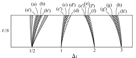
Figure 1: A schematic view of the phase diagram for $N=5$ and small $\varepsilon$. Inside the hatched regions $\mathcal{M}$ is unstable; and the dotted regions intend to represent finitely many disjoint hatched regions. Shaded regions are Arnold tongues with rotation numbers $n:m=1:2,\,1:1,\,2:1$ and $3:1$ from left to right.

Next, we present numerical results corroborating our theoretical results for $N=5$. The dynamics of infinitesimal perturbations transversal to the torus $(\delta\varphi_{1}\equiv\varphi_{1}-\varphi_{4},\delta\varphi_{2}\equiv\varphi_{2}-\varphi_{3})$ is governed by two linear equations:

$$\left\{\begin{array}[]{l}\displaystyle\dot{\delta\varphi_{1}}=-\frac{\varepsilon}{N}\cos(\varphi_{1}+\varphi_{2})(1+4\cos\varphi_{2})\delta\varphi_{1}+\frac{\varepsilon}{N}\left[\cos\varphi_{2}-\cos(\varphi_{1}+\varphi_{2})\right]\delta\varphi_{2},\\ \displaystyle\dot{\delta\varphi_{2}}=-\frac{\varepsilon}{N}\cos(\varphi_{1}+\varphi_{2})\sin^{2}(\varphi_{2}/2)\delta\varphi_{1}-\frac{\varepsilon}{N}\left[3\cos\varphi_{2}+2\cos(\varphi_{1}+\varphi_{2}))\right]\delta\varphi_{2}.\end{array}\right.$$ (16)

From these equations we calculate the TLEs ($\lambda_{\perp}^{(1)}\geq\lambda_{\perp}^{(2)}$) using the popular method by Benettin et al. [19]. In Fig. 2(a) we plot the TLEs for two values of $\varepsilon$ observing that: (i) TLEs are almost everywhere negative as expected from Theorem 1, (ii) TLEs for $\varepsilon=0.2$ and $0.4$ collapse when divided by $\varepsilon^{3}$, except if one enters in a locking region nor fulfilling the nonresonance condition in Th. 1 ($0:1$ locking in the leftmost part of the panel). Figure 3 shows a log-log plot of the TLEs as a function of $\varepsilon$ for a specific value of $\Delta_{1}$ (arbitrarily chosen with the constraint that the nonresonance condition is satisfied). We find a nice power law $\lambda_{\perp}^{(1,2)}=-|\lambda_{\perp}^{(1,2)}|\propto\varepsilon^{3}$, as expected from Theorem 1. In Figs. 2(b-e) we depict the largest TLE in four regions about lockings $1:2$, $1:1$, $2:1$, and $3:1$, finding that it becomes positive in short intervals as advanced in Theorem 2. These intervals match with the analytical expressions in Appendix.

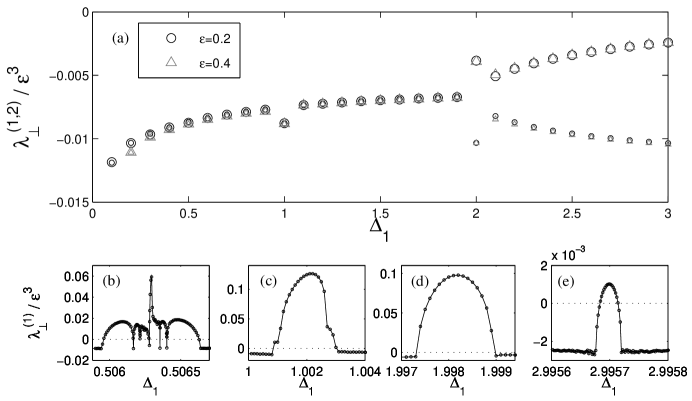
Figure 2: (a) Transverse Lyapunov exponents scaled by $\varepsilon^{3}$ as a function of $\Delta_{1}$ for $\varepsilon=0.2,0.4$ ($N=5$, $\Delta_{2}=1$). (b-e) Regions where the largest TLE becomes positive. (It is instructive to compare the panel (b) with the result in Fig. 9(a) obtained by the RG method.)

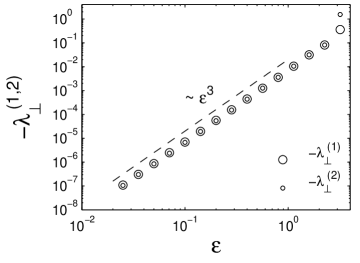
Figure 3: TLEs as a function of $\varepsilon$ for $N=5,\Delta_{2}=1$ and $\Delta_{1}=(1+\sqrt{5})/2$ (the golden mean).

4.3 $N=7$

For $N=7$ the system’s dimension is too large to perform a detailed analysis around all relevant resonances. But still the dimension is small enough to carry out intensive numerical simulations. We fixed $\Delta_{3}=1$ and measured the largest TLE at different values of $\Delta_{1}$ and $\Delta_{2}$. The initial condition in $\mathcal{M}$ was random (what should not be a problem if as we expect multistability is not common at small $\varepsilon$). In our simulations the coupling strength was $\varepsilon=0.3(N/2)\min_{i}{\Delta_{i}}$. This value of $\varepsilon$ is small enough to ensure the systems is far from synchronization, and at the same time large enough to make convergence times not exceedingly long for our computational resources. We may expect this value of $\varepsilon$ to capture the fundamental phenomenology as $\varepsilon\to 0$. The result is presented in Fig. 4, and shows that the dynamics on $\mathcal{M}$ is transversally stable in almost all the $\Delta_{1}$-$\Delta_{2}$ plane, except close to some resonances. These resonances should correspond to combinations of $\Delta_{i}$’s not fulfilling the nonresonance condition of Th. 1 (but also one may not exclude finite-$\varepsilon$ effects). The result is very much equivalent to the result for $N=5$, but with unstable regions organized around resonances involving three instead of two frequencies.

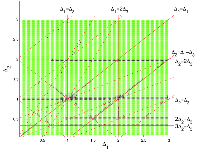
Figure 4: $\Delta_{1}$-$\Delta_{2}$ plane for $N=7$ with $\Delta_{3}=1$ and $\varepsilon=0.3(N/2)\min_{i}{\Delta_{i}}$. In the green regions the dynamics in $\mathcal{M}$ is transversally stable (i.e. there is an attractor $\mathcal{A}\subseteq\mathcal{M}$). Inside the black regions $\mathcal{M}$ is transversally unstable. (Red) lines indicate the loci of the most important resonances among $\{\Delta_{i}\}$.

5 Even $N$

In the symmetric Kuramoto model at small coupling the invariant torus $\mathcal{M}$ is almost always stable if the population size is odd. However, we show in this section that if $N$ is an even number $\mathcal{M}$ can be both stable and unstable in large regions of the parameter space spanned by the natural frequencies. We analyze the case $N=4$ in detail by means of the renormalization group (RG) method, and the case $N=6$ is studied using numerical calculations. Both cases share features that should be common to any even number $N\geq 4$.

5.1 $N=4$

When $N=4$, Eq. (2) with $\Delta_{1}=\Delta_{3}$ is written as

$$\left\{\begin{array}[]{l}\displaystyle\dot{\varphi}_{1}=\Delta_{1}+\frac{\varepsilon}{N}\Bigl{(}-2\sin\varphi_{1}+\sin\varphi_{2}\\ \quad\quad-\sin(\varphi_{1}+\varphi_{2})+\sin(\varphi_{2}+\varphi_{3})-\sin(\varphi_{1}+\varphi_{2}+\varphi_{3})\Bigr{)},\\ \displaystyle\dot{\varphi}_{2}=\Delta_{2}+\frac{\varepsilon}{N}\Bigl{(}-2\sin\varphi_{2}+\sin\varphi_{1}+\sin\varphi_{3}-\sin(\varphi_{1}+\varphi_{2})-\sin(\varphi_{2}+\varphi_{3})\Bigr{)},\\ \displaystyle\dot{\varphi}_{3}=\Delta_{1}+\frac{\varepsilon}{N}\Bigl{(}-2\sin\varphi_{3}+\sin\varphi_{2}\\ \quad\quad-\sin(\varphi_{2}+\varphi_{3})+\sin(\varphi_{1}+\varphi_{2})-\sin(\varphi_{1}+\varphi_{2}+\varphi_{3})\Bigr{)}.\\ \end{array}\right.$$ (17)

In this case, the invariant torus is given by the $2$-dimensional torus $\mathcal{M}=\{\varphi_{1}=\varphi_{3},\varphi_{2}\}$. Note that there will exist $n:m$ lockings on $\mathcal{M}$ like for $N=5$.

The linear ODE governing infinitesimal deviations off the torus ($\delta\varphi\equiv\varphi_{1}-\varphi_{3}$) is:

$$\dot{\delta\varphi}=-\frac{\varepsilon}{2}\left[\cos\varphi_{1}+\cos(\varphi_{1}+\varphi_{2})\right]\delta\varphi,$$ (18)

and it determines the TLE.

In what follows, we suppose $\Delta_{2}\neq 0$. By dividing Eq. (17) by $\Delta_{2}$, we can assume $\Delta_{2}=1$ without loss of generality.

Theorem 3. There exists a non-negative number $\varepsilon_{0}=\varepsilon_{0}(\Delta_{1})$ such that if $0<\varepsilon<\varepsilon_{0}$, the invariant torus $\mathcal{M}$ is asymptotically stable for $\Delta_{1}>1$ and unstable for $\Delta_{1}<1$. $\varepsilon_{0}(\Delta_{1})$ tends to zero as $\Delta_{1}\to 0,1/3,1/2,1,2,3,4$. The transverse Lyapunov exponent of $\mathcal{M}$ is of $O(\varepsilon^{5})$ if $0<\varepsilon<\varepsilon_{0}$.

A sketch of the strategy for proving this theorem is given in Sec. 7.3, while the detailed calculation is omitted. A schematic view of the phase diagram of Eq. (17) for small $\varepsilon$ is depicted in Fig. 5, in which there are no attractors $\mathcal{A}\subseteq\mathcal{M}$ in the hatched regions, and the $n:m$ locking solutions for $n:m=0:1,\,1:3,\,1:2,\,1:1,\,2:1,\,3:1$ and $4:1$ exist in the gray regions. In particular in the regions that are gray but not hatched, there are stable periodic orbits on $\mathcal{M}$. Asymptotic expansions with respect to $\varepsilon/N$ of boundary curves (i) to (u) and (i’) to (u’) in Fig. 5 are shown in Appendix.

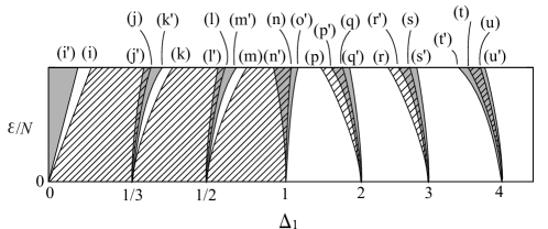
Figure 5: A schematic view of the phase diagram of Eq. (17) for small $\varepsilon$. There are no attractors $\mathcal{A}\subseteq\mathcal{M}$ in the hatched regions, and gray regions indicate the Arnold tongues.

We numerically calculated the TLE from Eq. (18), and Figs. 6 and 7 demonstrate that the TLE is $O(\varepsilon^{5})$ as stated in Theorem 3. $\mathcal{M}$ is mainly stable when $\Delta_{1}>1$. Like for $N=5$ there are “switching tongues” in which the stability of $\mathcal{M}$ is different from the dominant stability in its neighborhood. We do not show them in Fig. 6 not to overwhelm the reader with details. We note nevertheless that the analytical expressions (see Appendix) of boundary curves (i) to (u) have been corroborated by our numerical simulations.

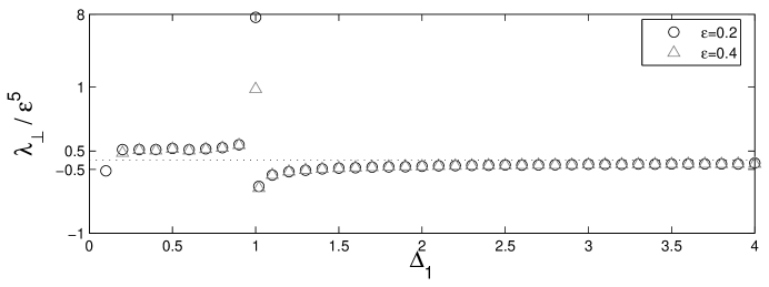
Figure 6: Transverse Lyapunov exponent scaled by $\varepsilon^{5}$ as a function of $\Delta_{1}$ for two values of $\varepsilon$ ($N=4$, $\Delta_{2}=1$). The scale of the y-axis is nonlinear to better discern the sign of the TLE. There is a perfect overlap of both data sets ($\varepsilon=0.2$ and $0.4$), except at frequency lockings $0:1$ and $1:1$. The stability change at $\Delta_{1}=1^{+}$ is very sharp but continuous.

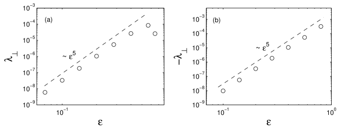
Figure 7: TLEs as a function of $\varepsilon$ for $N=4,\Delta_{2}=1$ and (a) $\Delta_{1}=(-1+\sqrt{5})/2$ (the inverse of the golden mean) (b) $\Delta_{1}=(1+\sqrt{5})/2$ (the golden mean). For the case (a) the invariant torus $\mathcal{M}$ is unstable while it is stable for (b) as stated in Theorem 3.

5.2 $N\geq 6$

We resort to extensive numerical simulations to study the case $N=6$, as we did already in Sec. 4.3 for $N=7$. Figure 8 summarizes the result of our simulations. There are regions with stable $\mathcal{M}$, and regions with unstable $\mathcal{M}$. Some low order resonances give rise to the border among these regions (analogously to the $\Delta_{1}=\Delta_{2}$ border in the $N=4$ case). Other resonances give rise to thin strips where the stability switches (again in good analogy to the $N=4$ case).

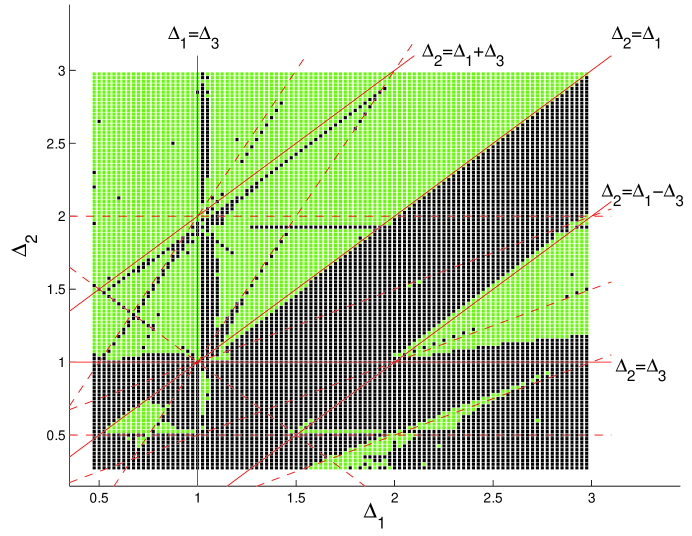
Figure 8: $\Delta_{1}$-$\Delta_{2}$ plane for $N=6$ with $\Delta_{3}=1$ and $\varepsilon=0.3(N/2)\min_{i}{\Delta_{i}}$. In the green regions the dynamics in $\mathcal{M}$ is transversally stable (i.e. there is an attractor $\mathcal{A}\subseteq\mathcal{M}$). Inside the black regions $\mathcal{M}$ is unstable. (Red) lines indicate the loci of the most important resonances among $\{\Delta_{i}\}$. In the regions with small $\Delta_{1}$ or $\Delta_{2}$ the convergence was too slow to guarantee accurate results (we have indications that typically the TLEs are $O(\varepsilon^{5})$ as for $N=4$).

If $\Delta_{1}$ is sufficiently large, oscillators $\theta_{1}$ and $\theta_{6}$ rotate so fast ($|\omega_{1}|\gg|\omega_{2,3}|$) that their influence on the other oscillators averages out. In this regime, (in)stability of the invariant torus is ruled by the four oscillators with the central frequencies. It may be perceived in Fig. 8 that for $\Delta_{1}\gg\Delta_{2,3}$ there is a switch of stability at $\Delta_{2}\gtrapprox\Delta_{3}=1$ in qualitative agreement with the $\Delta_{1}=\Delta_{2}+O(\varepsilon^{2})$ border in the $N=4$ case (the transition is not closer to $\Delta_{2}=1$ due to the finiteness of $\varepsilon$ and $\Delta_{1}$).

This simple argument based on the averaging method can be extended to an arbitrary (even) population size: In the limit $\Delta_{1}\to\infty$, Eq. (2) for $N=2M+2$ becomes equivalent to Eq. (2) for $N=2M$ because influence of $\varphi_{1}$ and $\varphi_{2M+1}$ on the other oscillators averages out. Thus by induction, we conclude that the situation of $N=4$ is typical for general even $N$; that is, regions of frequency space where $\mathcal{M}$ is stable and regions where it is unstable coexist in parameter space, none of them disappearing as $\varepsilon\to 0$. This property quite differs from the phase diagrams for odd $N$.

6 Discussion

One of the important results of our paper is the rather surprising fact that qualitative properties of the Kuramoto model (with symmetrically allocated natural frequencies) depend crucially on whether $N$ is odd or even. We establish precise mathematical criteria for the stability of the invariant torus $\mathcal{M}$. It is remarkable that in many cases this torus is asymptotically stable at arbitrarily small coupling. For $N=4,5$, we have completely uncovered stability changes caused by resonances.

The renormalization group method has been successfully used in this paper. In the literature, first- and second-order RG equations have been employed for constructing approximate solutions to weakly perturbed ODEs. In this paper, we have used this technique in the Kuramoto model up to third and fifth order for odd $N$ and for $N=4$, respectively. RG equations are quite helpful for studying the stability of invariant manifolds, and they provide as well the orders of magnitude of the transverse Lyapunov exponents.

In the context of coupled oscillators, the phenomenon known as ‘phase chaos’ consist in the appearance of a high-dimensional chaotic attractor [20, 21, 14] due to the interaction of phase variables (neutrally stable variables in the uncoupled limit). For the Kuramoto model it has been reported in [14] that (with a symmetric allocation of the natural frequencies) when increasing the coupling from zero the Lyapunov exponents split from a degenerate set at zero to a set of $[N/2]-1$ positive, $[N/2]-1$ negative, and 2 (3 if $N$ odd) zero Lyapunov exponents. In this paper we show that the invariant torus $\mathcal{M}$ is often stable in the small coupling limit. In contrast it is not proven yet that phase chaos indeed persists in the $\varepsilon\to 0$ limit. Here we note that our Theorem 1 applies in a finite range $0<\varepsilon<\varepsilon_{0}$ irrespective of how large $N$ is. Notice nevertheless that $\varepsilon_{0}\to 0$ as $N\to\infty$.

Other implications of our paper refer to numerical simulations. In this context our paper is particularly relevant because the Kuramoto model has been usually considered together with a symmetric frequency distribution of the natural frequencies, and in turn simulations, with a finite population size, are often carried out selecting frequencies that reflect the inherent symmetry of the frequency density. Our results also evidence the important role of resonances among the natural frequencies for the stability of the invariant torus $\mathcal{M}$. This must serve as a warning about the risks of using highly resonant frequencies when tackling generic properties of the system. In particular, it has become popular to consider evenly spaced natural frequencies ($\Delta_{i}=\Delta_{j}$ for all $i,j$), which is probably the most resonant case.

We may conjecture that the results reported here for the Kuramoto model (with a sinusoidal coupling function) should also be observed in a family of odd coupling functions. In fact, in the $N=3$ case, see Eq. (14), a family of functions shares stability and scaling of the transverse Lyapunov exponent. Nonetheless in what concerns the unstable regions (tongue-shaped for $N=5$) and their scaling one may expect important differences depending on the coupling function $f$. (We suspect this should be the case because of the similarity with the phase-locking regions, which depend on the harmonics of the interaction function [22].)

Finally, note that under a small enough symmetry-breaking perturbation $\mathcal{M}$ will get deformed into an invariant torus $\mathcal{M^{\prime}}$ with the same stability. Therefore our results may apply to situations where the symmetry is weakly broken.

7 Outline of the proofs of theorems

7.1 Brief review of the RG method

The renormalization group (RG) method is one of the singular perturbation methods for differential equations which provides approximate solutions as well as approximate invariant manifolds and their stability. Recently, it is shown that the RG method unifies and extends traditional singular perturbation methods, such as the averaging method, the multi-time scale method, the normal forms theory and so on. In this section, we give a brief review of the RG method following [17, 18] to prove Theorems 1 in the next subsection.

Consider the system of differential equations on a compact manifold $M$ of the form

$$\frac{dx}{dt}=\dot{x}=\varepsilon g_{1}(t,x)+\varepsilon^{2}g_{2}(t,x)+\varepsilon^{3}g_{3}(t,x)+\cdots,\,\,x\in M,$$ (19)

where $\varepsilon\in\mathbb{R}$ is a small parameter. For this system, we make the following assumption (A):

(A)   The vector fields $g_{i}(t,x),\,\,i=1,2,\cdots$ are $C^{1}$ with respect to time $t\in\mathbb{R}$ and $C^{\infty}$ with respect to $x\in M$. Further, $g_{i}$ are almost periodic functions with respect to $t$ uniformly in $x\in M$, the set of whose Fourier exponents has no accumulation points on $\mathbb{R}$.

In the case of the Kuramoto model (1), $M$ is an $N$-dimensional torus. Note that under the change of coordinates $\theta_{j}=x_{j}+\omega_{j}t$ and $\varphi_{j}=x_{j}+\Delta_{j}t$ systems (1) and (2), respectively, are transformed into the form of Eq. (19) with $g_{i}=0$ for $i\geq 2$, and satisfying the assumption (A).

Substitute $x=x_{0}+\varepsilon x_{1}+\varepsilon^{2}x_{2}+\cdots$ into the right hand side of Eq. (19) and expand it with respect to $\varepsilon$. We write the resultant as

$$\sum^{\infty}_{k=1}\varepsilon^{k}g_{k}(t,x_{0}+\varepsilon x_{1}+\varepsilon^{2}x_{2}+\cdots)=\sum^{\infty}_{k=1}\varepsilon^{k}G_{k}(t,x_{0},x_{1},\cdots,x_{k-1}).$$ (20)

For instance, $G_{1},G_{2}$ and $G_{3}$ are given by

$$G_{1}(t,x_{0}) = g_{1}(t,x_{0}),$$ (21)

$$G_{2}(t,x_{0},x_{1}) = \frac{\partial g_{1}}{\partial x}(t,x_{0})x_{1}+g_{2}(t,x_{0}),$$ (22)

$$G_{3}(t,x_{0},x_{1},x_{2}) = \frac{1}{2}\frac{\partial^{2}g_{1}}{\partial x^{2}}(t,x_{0})x_{1}^{2}+\frac{\partial g_{1}}{\partial x}(t,x_{0})x_{2}+\frac{\partial g_{2}}{\partial x}(t,x_{0})x_{1}+g_{3}(t,x_{0}),$$ (23)

respectively. With these $G_{i}$’s, we define the $C^{\infty}$ maps $R_{i},u^{(i)}_{t}:M\to M$ to be

$$R_{1}(y)=\lim_{t\to\infty}\frac{1}{t}\int^{t}\!G_{1}(s,y)ds,$$ (24)

$$u^{(1)}_{t}(y)=\int^{t}\!\left(G_{1}(s,y)-R_{1}(y)\right)ds,$$ (25)

and

$$R_{i}(y)=\lim_{t\to\infty}\frac{1}{t}\int^{t}\!\Bigl{(}G_{i}(s,y,u^{(1)}_{s}(y),\cdots,u^{(i-1)}_{s}(y))-\sum^{i-1}_{k=1}\frac{\partial u_{s}^{(k)}}{\partial y}(y)R_{i-k}(y)\Bigr{)}ds,$$ (26)

$$u^{(i)}_{t}(y)=\int^{t}\!\Bigl{(}G_{i}(s,y,u^{(1)}_{s}(y),\cdots,u^{(i-1)}_{s}(y))-\sum^{i-1}_{k=1}\frac{\partial u_{s}^{(k)}}{\partial y}(y)R_{i-k}(y)-R_{i}(y)\Bigr{)}ds,$$ (27)

for $i=2,3,\cdots$, respectively, where $\int^{t}$ denotes the indefinite integral, whose integral constants are fixed arbitrarily. We can prove that $R_{i}$ are well-defined (i.e. the limits exist) and $u^{(i)}_{t}$ are bounded in $t\in\mathbb{R}$. Along with $R_{i}$ and $u^{(i)}_{t}$, we define the $m$-th order RG equation for Eq. (19) to be

$$\dot{y}=\varepsilon R_{1}(y)+\varepsilon^{2}R_{2}(y)+\cdots+\varepsilon^{m}R_{m}(y),\,\,y\in M,$$ (28)

and the $m$-th order RG transformation $\alpha^{(m)}_{t}$ to be

$$\alpha^{(m)}_{t}(y)=y+\varepsilon u^{(1)}_{t}(y)+\cdots+\varepsilon^{m}u^{(m)}_{t}(y),\,\,y\in M.$$ (29)

Roughly speaking, we can show that the $m$-th order RG transformation $x=\alpha^{(m)}_{t}(y)$ brings the system (19) into the system of the form $\dot{y}=\varepsilon R_{1}(y)+\cdots+\varepsilon^{m}R_{m}(y)+\varepsilon^{m+1}S(t,x,\varepsilon)$, where $S$ is bounded in $t\in\mathbb{R}$. It means that the $m$-th order RG equation is $\varepsilon^{m+1}$-close to the original system (19) and thus it is useful to construct the flow of (19) approximately. Since the RG equation is an autonomous system while the original system (19) is not, to analyze the RG equation is easier than that of the original system. The next theorem is one of the fundamental theorems of the RG method.

Theorem A [17, 18]. Suppose that $R_{1}(y)=\cdots=R_{k-1}(y)=0$ and $\varepsilon^{k}R_{k}(y)$ is the first non-zero term in the RG equation. If the vector field $R_{k}(y)$ has a boundaryless compact normally hyperbolic invariant manifold $\mathcal{N}$, then for sufficiently small $\varepsilon>0$, Eq. (19) has an invariant manifold $\mathcal{N}_{\varepsilon}$, which is diffeomorphic to $\mathcal{N}$. In particular, stability of $\mathcal{N}_{\varepsilon}$ coincides with that of $\mathcal{N}$.

This theorem is used to investigate the stability of the invariant torus $\mathcal{M}$ and the $n:m$ locking solutions of the Kuramoto model.

7.2 Proof of Theorem 1

In this section, we give the proof of Theorem 1.

Proof of Theorem 1. Suppose that $N=2M-1$ is an odd number and $\omega_{i}$’s are allocated symmetrically as was assumed. Put $\theta_{i}=x_{i}+\omega_{i}t$ and rewrite Eq. (1) of the form of Eq. (19). If the natural frequencies satisfy the nonresonance condition (8), its third-order RG equation is given by

$$\left\{\begin{array}[]{l}\displaystyle\dot{y}_{M}=-\frac{16\varepsilon^{3}}{N^{3}}\sum_{k\neq M}\frac{1}{\omega_{k}^{2}}\sin(2y_{M}-y_{k}-y_{2M-k}),\\ \displaystyle\dot{y}_{i}=\frac{8\varepsilon^{2}}{N^{2}}\left(2\sum_{k\neq i}\frac{1}{\omega_{i}-\omega_{k}}-\frac{1}{\omega_{i}}\cos(y_{i}-2y_{M}+y_{2M-i})\right)\\ \displaystyle\quad+\frac{16\varepsilon^{3}}{N^{3}}\Biggl{(}\sum_{k\neq i,2M-i}\frac{1}{\omega_{i}^{2}-\omega_{k}^{2}}\sin(y_{i}-y_{k}-y_{2M-k}+y_{2M-i})\\ \displaystyle\quad-2\sum_{k\neq i,2M-i}\frac{1}{\omega_{i}(\omega_{i}-\omega_{k})}\sin(y_{i}-y_{k}-y_{2M-k}+y_{2M-i})\\ \displaystyle\quad+2\sum_{k\neq i,M}\frac{1}{\omega_{k}(\omega_{i}-\omega_{k})}\sin(2y_{M}-y_{k}-y_{2M-k})\\ \displaystyle\quad-\sum_{k\neq M,i,2M-i}\frac{1}{\omega_{k}(\omega_{i}+\omega_{k})}\sin(y_{i}-y_{k}-y_{2M-k}+y_{2M-i})\\ \displaystyle\quad-2\sum_{k\neq M,2M-i}\frac{1}{\omega_{i}(\omega_{i}+\omega_{k})}\sin(y_{i}-2y_{M}+y_{2M-i})\Biggr{)},\,\,\,\,(i\neq M).\end{array}\right.$$ (30)

Note that the first order term vanishes and the expansion begins with the second order term. Since the invariant torus $\mathcal{M}$ corresponds to the solution $y_{i}+y_{2M-i}=c$ (constant), we put $\phi_{i}=y_{i}+y_{2M-i}$ and $\phi_{M}=2y_{M}$. Then we obtain the system of $\phi_{i}$ :

$$\left\{\begin{array}[]{l}\displaystyle\dot{\phi}_{M}=-\frac{64\varepsilon^{3}}{N^{3}}\sum^{M-1}_{k=1}\frac{1}{\omega_{k}^{2}}\sin(\phi_{M}-\phi_{k}),\\ \displaystyle\dot{\phi}_{i}=\frac{32\varepsilon^{3}}{N^{3}}\Biggl{(}-\frac{1}{\omega_{i}^{2}}\sin(\phi_{i}-\phi_{M})-4\sum^{M-1}_{k\neq i}\frac{1}{\omega_{i}^{2}-\omega_{k}^{2}}\sin(\phi_{i}-\phi_{M})\\ \displaystyle\quad\quad\quad\quad+4\sum^{M-1}_{k\neq i}\frac{1}{\omega_{i}^{2}-\omega_{k}^{2}}\sin(\phi_{M}-\phi_{k})\Biggr{)},\,\,\,(i=1,\cdots,M-1).\end{array}\right.$$ (31)

Now that the second order term vanishes and Theorem A for $k=3$ is applicable to this system. We can prove that the eigenvalues of the Jacobian matrix of the r.h.s. of (31) at the fixed point $\phi_{i}=c\,\,(i=1,\cdots,M)$ have negative real parts, except a zero eigenvalue that results from the rotation invariance of Eq. (1) (or the degree of freedom of the constant $c$). A proof of this fact is outlined as follows:

Let $\mathcal{J}$ be the Jacobian matrix of the r.h.s. of (31) at the fixed point $\phi_{i}=c\,\,(i=1,\cdots,M)$. By using the cofactor expansion, it is easy to show that the characteristic polynomial of $\mathcal{J}$ is calculated as

$$\det\,(\lambda I-\frac{N^{3}}{32\varepsilon^{3}}\mathcal{J})=\lambda\cdot\det\,(\lambda I+\mathcal{A}_{M-1}),$$ (32)

where the matrix $\mathcal{A}_{M-1}$ is given as

$$\mathcal{A}_{M-1}=\left(\begin{array}[]{@{\,}cccc@{\,}}\displaystyle\frac{3}{\omega_{1}^{2}}+\sum^{M-1}_{k\neq 1}\frac{4}{\omega^{2}_{1}-\omega^{2}_{k}}&\displaystyle\frac{4}{\omega_{1}^{2}-\omega_{2}^{2}}+\frac{2}{\omega_{2}^{2}}&\cdots&\displaystyle\frac{4}{\omega_{1}^{2}-\omega_{M-1}^{2}}+\frac{2}{\omega_{M-1}^{2}}\\ \displaystyle\frac{4}{\omega_{2}^{2}-\omega_{1}^{2}}+\frac{2}{\omega_{1}^{2}}&\displaystyle\frac{3}{\omega_{2}^{2}}+\sum^{M-1}_{k\neq 2}\frac{4}{\omega^{2}_{2}-\omega^{2}_{k}}&\cdots&\displaystyle\frac{4}{\omega_{2}^{2}-\omega_{M-1}^{2}}+\frac{2}{\omega_{M-1}^{2}}\\ \vdots&\vdots&\ddots&\cdots\\ \displaystyle\frac{4}{\omega_{M-1}^{2}-\omega_{1}^{2}}+\frac{2}{\omega_{1}^{2}}&\displaystyle\frac{4}{\omega_{M-1}^{2}-\omega_{2}^{2}}+\frac{2}{\omega_{2}^{2}}&\cdots&\displaystyle\frac{3}{\omega_{M-1}^{2}}+\sum^{M-1}_{k\neq M-1}\frac{4}{\omega^{2}_{M-1}-\omega^{2}_{k}}\\ \end{array}\right).$$ (37)

Eq. (32) shows that $\mathcal{J}$ has a zero eigenvalue $\lambda=0$. Now it is sufficient to prove that all eigenvalues of $\mathcal{A}_{M-1}$ have positive real parts. To prove it, let

$$\lambda^{M-1}+f^{(M-2)}_{M-1}\lambda^{M-2}+f^{(M-3)}_{M-1}\lambda^{M-3}+\cdots+f^{(1)}_{M-1}\lambda+f^{(0)}_{M-1}=0$$ (38)

be the characteristic equation $\det(\lambda I-\mathcal{A}_{M-1})=0$ of $\mathcal{A}_{M-1}$. We show the inequalities $f^{(M-2)}_{M-1},f^{(M-4)}_{M-1}\cdots<0$ and $f^{(M-3)}_{M-1},f^{(M-5)}_{M-1}\cdots>0$ by induction on $M$. Since $f^{(i)}_{M-1}$ is invariant under the permutation of $\alpha_{1},\cdots,\alpha_{M-1}$, we can show that $f^{(i)}_{M-1}$ is of the form

$$f^{(i)}_{M-1}=b^{(i)}_{M-1}\frac{\sum_{i_{1}<\cdots<i_{k}}\alpha^{2}_{i_{1}}\alpha^{2}_{i_{2}}\cdots\alpha^{2}_{i_{k}}}{\alpha^{2}_{1}\alpha^{2}_{2}\cdots\alpha^{2}_{M-1}},\,\,b^{i}_{M-1}\in\mathbb{R}.$$ (39)

Since $\mathcal{A}_{M-1}\to\left(\begin{array}[]{@{\,}cc@{\,}}\mathcal{A}_{M-2}&0\\ \textstyle{*}&0\end{array}\right)$ as $\alpha_{M-1}\to 0$, $f^{(i)}_{M-1}\to f^{(i-1)}_{M-2}$ as $\alpha_{M-1}\to 0$. Now induction on $M$ proves the desired inequalities.

Thus, the solution $\phi_{i}=y_{i}+y_{2M-i}=c\,\,(i=1,\cdots,M)$ of the RG equation is asymptotically stable and this proves that the invariant torus $\mathcal{M}$ is asymptotically stable for small $\varepsilon>0$. Note that the degree of freedom of $c$ does not appear in the $\varphi_{j}$ coordinates [Eq. (2)]. $\blacksquare$

If $N=3(M=2)$, the nonresonance condition (8) is reduced to $\Delta_{1}\neq 0$ and Theorem 1 recovers the results obtained in Section 4.1.

7.3 Sketch of the proofs of Theorems 2 and 3

Theorems 2 and 3 are also proved by using the RG method though we need much harder analysis to obtain asymptotic expansions of the boundary lines in Figs. 1 and 5. In this section, we offer the strategy to prove Theorems and to derive the asymptotic expansions, which is also valid for any $N$.

In what follows, we assume $\Delta_{2}=1$ in Eqs. (15), (17) as was mentioned. Our strategy to prove Theorems 2 and 3, and to obtain boundary lines, is summarized as follows:

1. Put $\varphi_{i}=x_{i}+\Delta_{i}t$ and rewrite Eqs. (15) and (17) into the form of Eq. (19).

2. Derive the RG equations up to third-order for $N=5$ and to fifth-order for $N=4$. The forms of RG equations depend on $\Delta_{1}$. Find the set of values $\Delta_{1}$, which gives the nonresonance condition, at which RG equations take different forms from the others. We find that the nonresonance conditions are given by $\Delta_{1}\neq 0,1/2,1,2,3,4$ for $N=5$ and $\Delta_{1}\neq 0,1/3,1/2,1,2,3,4$ for $N=4$.

3. Investigate the stability of the invariant torus for the RG equation satisfying the nonresonance condition as was done in Sec. 7.2. In this step, the proof of Theorems 2 and 3 ends.

4. To find the Arnold tongues in Figs. 1 and 5, let $c_{0}$ be a resonance value obtained in step (ii). Put

   $$\Delta_{1}=c_{0}+c_{1}\varepsilon/N+c_{2}\varepsilon^{2}/N^{2}+\cdots$$ (40)

   in Eqs. (15) and (17), and derive the RG equations.

5. Investigate the stability of the invariant torus for the resultant RG equations and find values $c_{1},c_{2},\cdots$ at which the stability changes. Then, Eq. (40) gives an asymptotic expansion of a boundary line of the Arnold tongue emerging from $\Delta_{1}=c_{0}$ in the phase diagram.

In the next subsection, we calculate asymptotic expansions of boundary lines (a), (b), (a’) and (b’) in Fig. 1 to confirm this strategy for $N=5$ and $\Delta_{1}$ near $1/2$. Other expansions of boundary lines (c) to (u) and (c’) to (u’) in Figs. 1 and 5 are obtained analogously, and their derivation is omitted; the results are given in the Appendix.

7.4 Phase diagram near $\Delta_{1}=1/2$ for $N=5$

In this section, we derive asymptotic expansions of lines (a) and (b), as well as asymptotic expansions of lines (a’) and (b’), which are boundaries of the $1:2$ Arnold tongue for $N=5$. We also show that there are many disjoint unstable regions of $\mathcal{M}$ emerging from $\Delta_{1}/\Delta_{2}=1/2$ as is shown in Fig. 1.

To investigate the phase diagram of $N=5$ near $\Delta_{1}/\Delta_{2}=1/2$, put $\Delta_{2}=1,\,\Delta_{1}=1/2+c_{1}\varepsilon/N+c_{2}\varepsilon^{2}/N^{2}+\cdots$ and put $\varphi_{1}=x_{1}+t/2,\,\varphi_{2}=x_{2}+t,\,\varphi_{3}=x_{3}+t$ and $\varphi_{4}=x_{4}+t/2$ in Eq. (15). Then Eq. (15) takes the form of Eq. (19) and the RG method is applicable. The third-order RG equation for the system is given by

$$\frac{d}{dt}\left(\begin{array}[]{@{\,}c@{\,}}y_{1}\\ y_{2}\\ y_{3}\\ y_{4}\end{array}\right)=\frac{\varepsilon}{N}\left(\begin{array}[]{@{\,}c@{\,}}c_{1}\\ 0\\ 0\\ c_{1}\end{array}\right)$$ (49)

$$+\frac{\varepsilon^{2}}{N^{2}}\left(\begin{array}[]{@{\,}c@{\,}}\displaystyle-\frac{7}{2}+c_{2}-\frac{1}{2}\cos(y_{2}-y_{3})+\frac{1}{3}\cos(y_{1}+y_{2}-y_{3}-y_{4})\\[2.84544pt] \displaystyle\frac{1}{10}+\frac{1}{2}\cos(y_{2}-y_{3})\\[2.84544pt] \displaystyle\frac{1}{10}+\frac{1}{2}\cos(y_{2}-y_{3})\\[2.84544pt] \displaystyle-\frac{7}{2}+c_{2}-\frac{1}{2}\cos(y_{2}-y_{3})+\frac{1}{3}\cos(y_{1}+y_{2}-y_{3}-y_{4})\end{array}\right)$$ (54)

$$\!\!\!\!\!\!\!\!\!\!\!\!+\frac{\varepsilon^{3}}{N^{3}}\left(\begin{array}[]{@{\,}c@{\,}}\displaystyle\frac{26c_{1}}{3}+c_{3}-\frac{2c_{1}}{9}\cos(y_{1}+y_{2}-y_{3}-y_{4})-\frac{1}{2}\sin(2y_{1}-y_{2})\\[2.84544pt] \displaystyle\quad\quad\quad\quad-\frac{27}{20}\sin(y_{2}-y_{3})-\frac{1}{12}\sin(y_{2}-2y_{4})-\frac{77}{45}\sin(y_{1}+y_{2}-y_{3}-y_{4})\\[2.84544pt] \displaystyle-\frac{96c_{1}}{25}-2\sin(2y_{1}-y_{2})+\frac{1}{12}\sin(2y_{1}-y_{3})+\frac{1}{20}\sin(y_{2}-y_{3})\\[2.84544pt] \displaystyle\quad\quad\quad\quad+\frac{1}{6}\sin(y_{2}-2y_{4})-\frac{3}{2}\sin(y_{3}-2y_{4})+\frac{26}{45}\sin(y_{1}+y_{2}-y_{3}-y_{4})\\[2.84544pt] \displaystyle-\frac{96c_{1}}{25}+\frac{3}{2}\sin(2y_{1}-y_{2})-\frac{1}{6}\sin(2y_{1}-y_{3})-\frac{1}{20}\sin(y_{2}-y_{3})\\[2.84544pt] \displaystyle\quad\quad\quad\quad-\frac{1}{12}\sin(y_{2}-2y_{4})+2\sin(y_{3}-2y_{4})-\frac{26}{45}\sin(y_{1}+y_{2}-y_{3}-y_{4})\\[2.84544pt] \displaystyle\frac{26c_{1}}{3}+c_{3}-\frac{2c_{1}}{9}\cos(y_{1}+y_{2}-y_{3}-y_{4})+\frac{1}{12}\sin(2y_{1}-y_{3})\\[2.84544pt] \displaystyle\quad\quad\quad\quad+\frac{27}{20}\sin(y_{2}-y_{3})+\frac{1}{2}\sin(y_{3}-2y_{4})+\frac{77}{45}\sin(y_{1}+y_{2}-y_{3}-y_{4})\end{array}\right).$$ (63)

This system has the solution $y_{1}=y_{4},\,y_{2}=y_{3}$, which corresponds to the invariant torus $\mathcal{M}$. The linearized equation for Eq. (63) along the solution $y_{1}=y_{4},\,y_{2}=y_{3}$ is given as

$$\frac{d}{dt}\left(\begin{array}[]{@{\,}c@{\,}}\delta y_{1}\\ \delta y_{2}\end{array}\right)=\frac{\varepsilon^{3}}{N^{3}}\left(\begin{array}[]{ll}\displaystyle-\frac{7}{90}(44+15\cos y)&\displaystyle-\frac{551}{90}+\frac{5\cos y}{12}\\ \displaystyle\frac{52}{45}-\frac{13\cos y}{2}&\displaystyle\frac{113}{90}+\frac{15\cos y}{4}\end{array}\right)\left(\begin{array}[]{@{\,}c@{\,}}\delta y_{1}\\ \delta y_{2}\end{array}\right),$$ (70)

where $\delta y_{1}=y_{1}-y_{4},\delta y_{2}=y_{2}-y_{3}$, and where $y=y(t)$ is a solution of the equation

$$\frac{dy}{dt}=\frac{2\varepsilon}{N}c_{1}+\frac{\varepsilon^{2}}{N^{2}}\left(2c_{2}-\frac{119}{15}\right)+\frac{\varepsilon^{3}}{N^{3}}\left(\frac{4664}{225}c_{1}+2c_{3}-\frac{1}{4}\sin y\right),$$ (71)

which is obtained by putting $2y_{1}-y_{2}=y,\,y_{4}=y_{1},\,y_{3}=y_{2}$ in Eq. (63). The existence of $1:2$ locking corresponds to the existence of a stable fixed point of $y$, and the stability of the invariant torus $\mathcal{M}$ is maps to the stability of the trivial solution $\delta y_{1}=\delta y_{2}=0$ in Eq. (70). Stability depends on the coefficients $c_{i}$ in Eq. (71).

1. When $c_{1}\neq 0$, then we can apply the averaging method to Eqs. (70, 71). Averaged with respect to $y$, Eq. (70) is rewritten as

   $$\frac{d}{dt}\left(\begin{array}[]{@{\,}c@{\,}}\delta y_{1}\\ \delta y_{2}\end{array}\right)=\frac{\varepsilon^{3}}{N^{3}}\left(\begin{array}[]{ll}-154/45&-551/90\\ 52/45&113/90\end{array}\right)\left(\begin{array}[]{@{\,}c@{\,}}\delta y_{1}\\ \delta y_{2}\end{array}\right).$$ (72)

   It is easy to verify that the trivial solution of this system is stable because the eigenvalues of the matrix in the right hand side are given by $(-13\pm\sqrt{231}i)/12$. It proves that the invariant torus $\mathcal{M}$ is stable if $c_{1}\neq 0$.

2. When $c_{1}=0$ and $c_{2}\neq 119/30$, we can apply the averaging again to obtain Eq. (72) what proves that $\mathcal{M}$ is stable in the same way as (i).

3. When $c_{1}=0$ and $c_{2}=119/30$, Eq. (71) becomes

   $$\frac{dy}{dt}=\frac{2\varepsilon^{3}}{N^{3}}\left(c_{3}-\frac{1}{8}\sin y\right).$$ (73)

   1. If $|c_{3}|<1/8$, the above equation has a stable fixed point $y=y_{*}$ such that $\sin y_{*}=8c_{3},\,\cos y_{*}=(1-64c_{3}^{2})^{1/2}$. It corresponds to the $1:2$ locking solution because $y=2y_{1}-y_{2}$. The disappearance of the fixed point at $|c_{3}|=1/8$ marks the boundaries of the Arnold tongue: asymptotic expansions (a’) and (b’) in Appendix. It is easy to investigate the stability of the trivial solution of the linearized equation (70) with constant coefficients. Indeed, we can show that the trivial solution is unstable if and only if

      $$|c_{3}|<\frac{1}{4}\left(\frac{8681209}{17391218+5894\sqrt{8738809}}\right)^{1/2}=0.124838\ldots$$ (74)

      And this proves that the invariant torus $\mathcal{M}$ is unstable in the region surrounded by the lines (a) and (b) given in Appendix.

   2. If $|c_{3}|>1/8$, the linearized equation (70) is a linear system with a time periodic coefficient. It is well known that stability of a trivial solution of such a system is determined by the Floquet exponents although we can not calculate them analytically in general. We examine the stability of the trivial solution of Eq. (70) by calculating the Lyapunov exponents numerically.

      

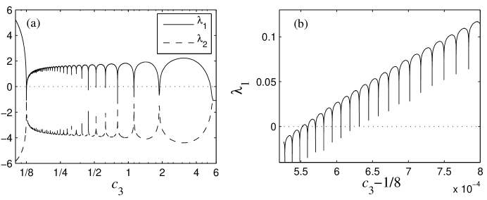
      Figure 9: (a) Lyapunov exponents ($\lambda_{1}\geq\lambda_{2}$) of system (70) forced by (73) ($\varepsilon/N=1$ is arbitrarily adopted). In the interval $0.125552\ldots<c_{3}<5.3695\ldots$, $\lambda_{1}$ is mostly positive except at hundreds of narrow windows where it becomes negative (to coincide with $\lambda_{2}$). (b) In this panel we see how $\lambda_{1}$ presents dips that accumulate at $c_{3}=1/8$; the dips are so narrow that the sampling is not able to resolve the intervals where $\lambda_{1}=\lambda_{2}$.

      Figure 9 shows that there are many disjoint intervals of $c_{3}$ on which the trivial solution of Eq. (70) is unstable. It proves that there are many disjoint unstable regions of the invariant torus $\mathcal{M}$ emerging from $\Delta_{1}=1/2$. These unstable regions are inside the region limited by $\Delta_{1}=\frac{1}{2}+\frac{119}{30}\frac{\varepsilon^{2}}{N^{2}}+0.125552\frac{\varepsilon^{3}}{N^{3}}+O(\varepsilon^{4})$ and $\Delta_{1}=\frac{1}{2}+\frac{119}{30}\frac{\varepsilon^{2}}{N^{2}}+5.3695\frac{\varepsilon^{3}}{N^{3}}+O(\varepsilon^{4})$; and inside a twin region with opposite signs in the cubic terms (dotted regions in Fig. 1).

Appendix : Asymptotic expansions of boundary curves in Fig. 1 ($N=5$) and Fig. 5 ($N=4$)

Asymptotic expansions in $\varepsilon$ of lines (a) to (h) in Fig. 1, which divide stable regions and unstable regions of the invariant torus $\mathcal{M}$ for $N=5$, are

$$(\rm{a,b}) \Delta_{1}=\frac{1}{2}+\frac{119}{30}\frac{\varepsilon^{2}}{N^{2}}\mp\frac{1}{4}\left(\frac{8681209}{17391218+5894\sqrt{8738809}}\right)^{1/2}\frac{\varepsilon^{3}}{N^{3}}+O(\varepsilon^{4}),$$

$$(\rm{c}) \Delta_{1}=1+\frac{2}{3}\frac{\varepsilon^{2}}{N^{2}}-\frac{689009}{362880}\frac{\varepsilon^{4}}{N^{4}}+O(\varepsilon^{5}),$$

$$(\rm{d}) \Delta_{1}=1+\frac{5}{3}\frac{\varepsilon^{2}}{N^{2}}+\left(\frac{1027631}{241920}+k_{1}\right)\frac{\varepsilon^{4}}{N^{4}}+O(\varepsilon^{5}),$$

$$(\rm{e}) \Delta_{1}=2-\frac{5}{3}\frac{\varepsilon^{2}}{N^{2}}-\frac{139753}{241920}\frac{\varepsilon^{4}}{N^{4}}+O(\varepsilon^{5}),$$

$$(\rm{f}) \Delta_{1}=2-\frac{2}{3}\frac{\varepsilon^{2}}{N^{2}}+\left(-\frac{136655}{48384}+k_{2}\right)\frac{\varepsilon^{4}}{N^{4}}+O(\varepsilon^{5}),$$

$$(\rm{g,h}) \Delta_{1}=3-\frac{161}{60}\frac{\varepsilon^{2}}{N^{2}}\mp\left(\frac{191\sqrt{18481}-24281}{28800}\right)^{1/2}\frac{\varepsilon^{3}}{N^{3}}+O(\varepsilon^{4}),$$

where $k_{1}$ and $k_{2}$ are some positive constant which are not obtained analytically.

Asymptotic expansions of boundaries (a’) to (h’) of the $n:m$ Arnold tongues in Fig. 1 are

$$(\rm{a^{\prime},b^{\prime}}) \Delta_{1}=\frac{1}{2}+\frac{119}{30}\frac{\varepsilon^{2}}{N^{2}}\mp\frac{1}{8}\frac{\varepsilon^{3}}{N^{3}}+O(\varepsilon^{4}),$$

$$(\rm{c^{\prime}}) \Delta_{1}=1+\frac{2}{3}\frac{\varepsilon^{2}}{N^{2}}-\frac{684751}{241920}\frac{\varepsilon^{4}}{N^{4}}+O(\varepsilon^{5}),$$

$$(\rm{d^{\prime}}) \Delta_{1}=1+\frac{5}{3}\frac{\varepsilon^{2}}{N^{2}}+\frac{1027631}{241920}\frac{\varepsilon^{4}}{N^{4}}+O(\varepsilon^{5}),$$

$$(\rm{e^{\prime}}) \Delta_{1}=2-\frac{5}{3}\frac{\varepsilon^{2}}{N^{2}}-\frac{291373}{241920}\frac{\varepsilon^{4}}{N^{4}}+O(\varepsilon^{5}),$$

$$(\rm{f^{\prime}}) \Delta_{1}=2-\frac{2}{3}\frac{\varepsilon^{2}}{N^{2}}-\frac{136655}{48384}\frac{\varepsilon^{4}}{N^{4}}+O(\varepsilon^{5}),$$

$$(\rm{g^{\prime},h^{\prime}}) \Delta_{1}=3-\frac{161}{60}\frac{\varepsilon^{2}}{N^{2}}\mp\frac{1}{3}\frac{\varepsilon^{3}}{N^{3}}+O(\varepsilon^{4}).$$

Asymptotic expansions of the lines (i) to (u) in Fig. 5, which divide stable regions and unstable regions of the invariant torus $\mathcal{M}$ for $N=4$, are

$$(\rm{i}) \Delta_{1}=\frac{58}{\sqrt{805}}\frac{\varepsilon}{N}+O(\varepsilon^{2}),$$

$$(\rm{j}) \Delta_{1}=\frac{1}{3}+\frac{193}{30}\frac{\varepsilon^{2}}{N^{2}}-\frac{6767219}{84000}\frac{\varepsilon^{4}}{N^{4}}+\frac{102957740948201549}{59535676200000}\frac{\varepsilon^{6}}{N^{6}}+O(\varepsilon^{7}),$$

$$(\rm{k}) \Delta_{1}=\frac{1}{3}+\frac{193}{30}\frac{\varepsilon^{2}}{N^{2}}-\frac{145573959475337}{3308633832000}\frac{\varepsilon^{4}}{N^{4}}+O(\varepsilon^{5}),$$

$$(\rm{l}) \Delta_{1}=\frac{1}{2}+\frac{23}{6}\frac{\varepsilon^{2}}{N^{2}}+2\frac{\varepsilon^{3}}{N^{3}}-\frac{202777}{7560}\frac{\varepsilon^{4}}{N^{4}}-\frac{72568}{1575}\frac{\varepsilon^{5}}{N^{5}}+O(\varepsilon^{6}),$$

$$(\rm{m}) \Delta_{1}=\frac{1}{2}+\frac{593}{106}\frac{\varepsilon^{2}}{N^{2}}+O(\varepsilon^{3}),$$

$$(\rm{n}) \Delta_{1}=1+\frac{4}{3}\frac{\varepsilon^{2}}{N^{2}}-\frac{24289}{4320}\frac{\varepsilon^{4}}{N^{4}}+O(\varepsilon^{5}),$$

$$(\rm{p}) \Delta_{1}=2-\frac{168449}{47505}\frac{\varepsilon^{2}}{N^{2}}+O(\varepsilon^{3}),$$

$$(\rm{q}) \Delta_{1}=2-\frac{47}{15}\frac{\varepsilon^{2}}{N^{2}}+\frac{1}{4}\frac{\varepsilon^{3}}{N^{3}}-\frac{241399}{378000}\frac{\varepsilon^{4}}{N^{4}}+\frac{1339}{56700}\frac{\varepsilon^{5}}{N^{5}}+O(\varepsilon^{6}),$$

$$(\rm{r}) \Delta_{1}=3-\frac{239}{42}\frac{\varepsilon^{2}}{N^{2}}-\frac{168549449269}{41374295424}\frac{\varepsilon^{4}}{N^{4}}+O(\varepsilon^{5}),$$

$$(\rm{s}) \Delta_{1}=3-\frac{239}{42}\frac{\varepsilon^{2}}{N^{2}}-\frac{11279063}{3259872}\frac{\varepsilon^{4}}{N^{4}}-\frac{12019873522646189}{6354207699840000}\frac{\varepsilon^{6}}{N^{6}}+O(\varepsilon^{7}),$$

$$(\rm{t,u}) \Delta_{1}=4-\frac{719}{90}\frac{\varepsilon^{2}}{N^{2}}-\frac{1658470531}{265356000}\frac{\varepsilon^{4}}{N^{4}}\mp\frac{\sqrt{63584702081}}{3302208}\frac{\varepsilon^{5}}{N^{5}}+O(\varepsilon^{6}).$$

Asymptotic expansions of boundaries (i’) to (u’) of the $n:m$ Arnold tongues in Fig. 5 are

$$(\rm{i}^{\prime}) \Delta_{1}=2\frac{\varepsilon}{N}+O(\varepsilon^{2}),$$

$$(\rm{j^{\prime}}) \Delta_{1}=\frac{1}{3}+\frac{193}{30}\frac{\varepsilon^{2}}{N^{2}}-\frac{8249819}{84000}\frac{\varepsilon^{4}}{N^{4}}+O(\varepsilon^{5}),$$

$$(\rm{k^{\prime}}) \Delta_{1}=\frac{1}{3}+\frac{193}{30}\frac{\varepsilon^{2}}{N^{2}}-\frac{6767219}{84000}\frac{\varepsilon^{4}}{N^{4}}+\frac{1286745722182601}{742041300000}\frac{\varepsilon^{6}}{N^{6}}+O(\varepsilon^{7}),$$

$$(\rm{l^{\prime}}) \Delta_{1}=\frac{1}{2}+\frac{23}{6}\frac{\varepsilon^{2}}{N^{2}}-2\frac{\varepsilon^{3}}{N^{3}}+O(\varepsilon^{4}),$$

$$(\rm{m^{\prime}}) \Delta_{1}=\frac{1}{2}+\frac{23}{6}\frac{\varepsilon^{2}}{N^{2}}+2\frac{\varepsilon^{3}}{N^{3}}-\frac{202777}{7560}\frac{\varepsilon^{4}}{N^{4}}-\frac{7752}{175}\frac{\varepsilon^{5}}{N^{5}}+O(\varepsilon^{6}),$$

$$(\rm{n^{\prime}}) \Delta_{1}=1-\frac{2}{3}\frac{\varepsilon^{2}}{N^{2}}+O(\varepsilon^{4}),$$

$$(\rm{o^{\prime}}) \Delta_{1}=1+\frac{4}{3}\frac{\varepsilon^{2}}{N^{2}}-\frac{17029}{4320}\frac{\varepsilon^{4}}{N^{4}}+O(\varepsilon^{5}),$$

$$(\rm{p^{\prime}}) \Delta_{1}=2-\frac{47}{15}\frac{\varepsilon^{2}}{N^{2}}-\frac{1}{4}\frac{\varepsilon^{3}}{N^{3}}+O(\varepsilon^{4}),$$

$$(\rm{q^{\prime}}) \Delta_{1}=2-\frac{47}{15}\frac{\varepsilon^{2}}{N^{2}}+\frac{1}{4}\frac{\varepsilon^{3}}{N^{3}}-\frac{241399}{378000}\frac{\varepsilon^{4}}{N^{4}}+\frac{5027}{6300}\frac{\varepsilon^{5}}{N^{5}}+O(\varepsilon^{6}),$$

$$(\rm{r^{\prime}}) \Delta_{1}=3-\frac{239}{42}\frac{\varepsilon^{2}}{N^{2}}-\frac{12094031}{3259872}\frac{\varepsilon^{4}}{N^{4}}+O(\varepsilon^{5}),$$

$$(\rm{s^{\prime}}) \Delta_{1}=3-\frac{239}{42}\frac{\varepsilon^{2}}{N^{2}}-\frac{11279063}{3259872}\frac{\varepsilon^{4}}{N^{4}}-\frac{68218740201013}{50833661598720}\frac{\varepsilon^{6}}{N^{6}}+O(\varepsilon^{7}),$$

$$(\rm{t^{\prime},u^{\prime}}) \Delta_{1}=4-\frac{719}{90}\frac{\varepsilon^{2}}{N^{2}}-\frac{1658470531}{265356000}\frac{\varepsilon^{4}}{N^{4}}\mp\frac{5}{64}\frac{\varepsilon^{5}}{N^{5}}+O(\varepsilon^{6}).$$

References

- [1] Y. Kuramoto, Chemical Oscillations, Waves, and Turbulence, Springer-Verlag, Berlin, 1984.
- [2] S. H. Strogatz, From Kuramoto to Crawford: exploring the onset of synchronization in populations of coupled oscillators, Physica D 143 (2000) 1–20.
- [3] J. A. Acebrón, L. L. Bonilla, C. J. P. Vicente, F. Ritort, R. Spigler, The Kuramoto model: a simple paradigm for synchronization phenomena, Rev. Mod. Phys. 77 (2005) 137–185.
- [4] A. Pikovsky, M. Rosenblum, J. Kurths, Synchronization: A Universal Concept in Nonlinear Sciences, Cambridge University Press, Cambridge, 2001.
- [5] S. C. Manrubia, S. S. Mikhailov, D. H. Zanette, Emergence of Dynamical Order, World Scientific, Singapore, 2004.
- [6] H. Daido, Intrinsic fluctuations and a phase transition in a class of large populations of interacting oscillators, J. Stat. Phys. 60 (1990) 753–800.
- [7] N. J. Balmforth, R. Sassi, A shocking display of synchrony, Physica D 143 (2000) 21–55.
- [8] H. Hong, H. Chaté, H. Park, L.-H. Tang, Entrainment transition in populations of random frequency oscillators, Phys. Rev. Lett. 99 (18) (2007) 184101.
- [9] E. J. Hildebrand, M. A. Buice, C. C. Chow, Kinetic theory of coupled oscillators, Phys. Rev. Lett. 98 (5) (2007) 054101.
- [10] M. A. Buice, C. C. Chow, Correlations, fluctuations, and stability of a finite-size network of coupled oscillators, Phys. Rev. E 76 (3) (2007) 031118.
- [11] Y. Maistrenko, O. Popovych, O. Burylko, P. A. Tass, Mechanism od desynchronization in the finite-dimensional Kuramoto model, Phys. Rev. Lett. 93 (2004) 084102.
- [12] Y. L. Maistrenko, O. V. Popovych, P. A. Tass, Desynchronization and chaos in the Kuramoto model, Lect. Notes in Phys. 671 (2005) 285–306.
- [13] Y. L. Maistrenko, O. V. Popovych, P. A. Tass, Chaotic attractor in the Kuramoto model, Int. J. of Bif. and Chaos 15 (2005) 3457–3466.
- [14] O. V. Popovych, Y. L. Maistrenko, P. A. Tass, Phase chaos in coupled oscillators, Phys. Rev. E 71 (2005) 065201.
- [15] L. Y. Chen, N. Goldenfeld, Y. Oono, Renormalization group theory for global asymptotic analysis, Phys. Rev. Lett. 73 (10) (1994) 1311–1315.
- [16] L.-Y. Chen, N. Goldenfeld, Y. Oono, Renormalization group and singular perturbations: Multiple scales, boundary layers, and reductive perturbation theory, Phys. Rev. E 54 (1) (1996) 376–394.
- [17] H. Chiba, approximation of vector fields based on the renormalization group method, SIAM J. Appl. Dyn. Syst. 7 (2008) 895–932.
- [18] H. Chiba, Extension and unification of singular perturbation methods for ODEs based on the renormalization group method, (submitted).
- [19] G. Benettin, L. Galgani, A. Giorgilli, J.-M. Strelcyn, Lyapunov characteristic exponents for smooth dynamical systems and for Hamiltonian systems, Meccanica 15 (1980) 9.
- [20] D. Topaj, A. Pikovsky, Reversibility vs. synchronization in oscillator lattices, Physica D 170 (2002) 118–130.
- [21] Z. Liu, Y.-C. Lai, M. A. Matías, Universal scaling of Lyapunov exponents in coupled chaotic oscillators, Phys. Rev. E 67 (4) (2003) 045203.
- [22] O. G. Galkin, Phase-locking for dynamical systems on the torus and perturbation theory for Mathieu-type problems, J. Nonlinear Sci. 4 (1994) 127–156.