Quantum Hall droplet laterally coupled to a quantum ring

Abstract

We study a two-dimensional cylindrically-symmetric electron droplet separated from a surrounding electron ring by a tunable barrier using the exact diagonalization method. The magnetic field is assumed strong so that the electrons become spin-polarized and reside on the lowest Fock-Darwin band. We calculate the ground state phase diagram for 6 electrons. At weak coupling, the phase diagram exhibits a clear diamond structure due to the blockade caused by the angular momentum difference between the two systems. We find separate excitations of the droplet and the ring as well as the transfer of charge between the two parts of the system. At strong coupling, interactions destroy the coherent structure of the phase diagram, while individual phases are still heavily affected by the potential barrier.

I Introduction

Fractional quantum Hall (FQH) fluids are observed at low temperature in clean two-dimensional electron gas exposed to a perpendicular magnetic field.tsui ; laughlin ; jain Each of them possesses unique topological order and is characterized by a number of universal invariants such as the Hall conductance and the fractional charges and braiding statistics of the elementary quasiparticle excitations.wen_adv ; nayak In quantum Hall droplets realizable in semiconductor quantum dots, a microscopic number of electrons forms an analogous correlated fluid. While the universalities are no longer exactly valid, the system can be accurately studied by various non-perturbative numerical methods combined with the understanding of the quantum Hall effects.henri ; saarikoski_pf

In this paper, we investigate a cylindrically-symmetric electron droplet separated from a surrounding electron ring by a tunable barrier. The magnetic field is assumed strong so that the electrons are spin-polarized and reside on the lowest Fock-Darwin band. fock We find the ground state phase diagram for 6 electrons. When the ring and dot are weakly coupled, the ground state angular momenta form a diamond structure, following from the conservation of the total angular momentum in the combined system. This structure is gradually lost as the systems become strongly coupled. Finally, the effects of the potential wall when all the electrons are in the dot are analyzed.

An earlier theoretical study of transport properties of a similar ring-dot structure, albeit with weaker magnetic field, showed evidence of a transport blockade due to the system geometry.guclu Later it was suggested that due to the piecewise linear dependence of the singlet-triplet splitting, a ring-dot geometry would be a good candidate for a realization of magnetic field controllable pair of spin qubits.szafran We are unaware of experiments conducted with this type of concentric laterally coupled quantum-dot-quantum-ring systems. However, in a recent experiment with coupled concentric quantum rings, Aharonov-Bohm periods matching the radius of both rings were found.muhle Persistent current and capacitance oscillations in side coupled and embedded ring-dot systems have been studied.buttiker Interference and phase phenomena in a quantum dot molecule embedded in a ring interferometer have been experimented,ihn and the Fano effect in a side coupled quantum ring and dot has been experimentally observed.fuhrer

The rest of the paper is organized as follows. In Section II, we present the model and the numerical methods. Section III contains the results summarized in Section IV.

II Model and method

The system is modelled by an effective-mass Hamiltonian

$$H=\sum^{N}_{i=1}\left[\frac{({\bf p}_{i}+\frac{e}{c}{\bf A}_{i})^{2}}{2m^{*}}+V(r_{i})\right]+\sum_{i<j}\frac{e^{2}}{\epsilon r_{ij}}\ ,$$ (1)

where $N$ is the number of electrons, and ${\bf A}$ is the vector potential of the homogeneous magnetic field ${\bf B}$ perpendicular to the plane. The material dependent parameters are $m^{*}=0.067m_{e}$, the effective mass of an electron, and $\epsilon=12.7$ (CGS), the dielectric constant of GaAs semiconductor medium. The confinement potential and the barrier between the quantum dot and quantum ring are given by

$$V(r)=\frac{m^{*}\omega_{0}^{2}r^{2}}{2}+C\delta(r-r_{0})\ .$$ (2)

The potential barrier separating the two subsystems is approximated by a delta function at radius $r_{0}$ scaled by strength $C$. In this model that aims to capture the essential properties, we neglect the effects of small thickness of the sampletolo and screening by near-by metallic gates to the Coulomb interaction.

In the calculations, we set the confinement strength $\hbar\omega_{0}$ to $2\,{\rm meV}$ as its scaling should merely shift the ranges of magnetic fields for different phases. Lengths are written in units of oscillator length $l=\sqrt{\hbar/(m^{*}\omega)}$, where $\omega=\sqrt{\omega_{0}^{2}+(\omega_{c}/2)^{2}}$ and $\omega_{c}=eB/(m^{*}c)$ is the cyclotron frequency. The ground state of Eq. (1) is solved by constructing the many-body Hamiltonian matrix in the basis of spin-polarized lowest Fock-Darwin band and finding its lowest eigenstate by the Lanczos diagonalization. The former constitutes a Landau level projection, an approximation that is valid at the high magnetic field regime.siljamaki

The single-particle wave functions in oscillator units read

$$\langle z|m\rangle=\tfrac{1}{\sqrt{\pi m!}}z^{m}e^{-z\bar{z}/2}\ ,\ \ m\geqslant 0\ ,$$ (3)

where $z=x+iy$. The non-trivial quantities are the interaction matrix elements $\langle m^{\prime},n^{\prime}|1/r_{12}|m,n\rangle$. Utilizing the angular momentum conservation $m^{\prime}+n^{\prime}=m+n$, these can be written in terms of

$$M^{l}_{mn}=\langle m+l,n|1/r_{12}|m,n+l\rangle\ ,\ \ l,m,n\geqslant 0\ ,$$ (4)

for which a particularly stable analytic formula has been derived by Tsiper. tsiper_c

The first step in our analysis is to select the tunable parameters and calculate the ground state angular momentum phase diagram. For illustrational reasons, we content ourselves to two continuous parameters, the magnetic field $B$ and the position of the potential barrier $r_{0}$. By application of the following scaling trick, which corresponds to curvilinear representation of the tunable parameters, the number of Lanczos diagonalizations needed to compute a phase diagram can be greatly reduced.

Up to a constant shift, the energy $E$ of the ground state $|\Psi\rangle$ of the ring-dot system for a fixed total angular momentum $M$ reads

$$E=\left(\hbar\omega-\frac{\hbar\omega_{c}}{2}\right)M+\hbar\omega\left[\frac{CV_{B}}{\hbar\omega l^{2}}+\frac{l}{a_{*}}V_{C}\right]\ ,$$ (5)

where $a_{*}=4\pi\epsilon\hbar^{2}/(m^{*}e^{2})$ is the effective Bohr radius, $V_{B}=\langle\Psi|\sum_{i}\delta(r_{i}-r_{0})|\Psi\rangle$ in units of $1/l^{2}$, and $V_{C}=\langle\Psi|\sum_{i<j}1/{r_{ij}}|\Psi\rangle$ in units of $1/l$. Hence, we find it convenient to scale the strength of the potential barrier as $C=(l^{3}/a_{*})\hbar\omega\beta$ (see Fig. 1) with a dimensionless potential barrier strength parameter $\beta$, fixed for a given phase diagram. The ground state phase diagram is then efficiently computed by performing the exact diagonalization at each angular momentum value at each position (in units of $l$) of the barrier, after which the magnetic field dependence of the energies can be easily obtained without need for doing the diagonalization at each magnetic field value. After the angular momenta of adjacent phases are determined, the exact value of the magnetic field $B$ at the boundary is solved from an algebraic equation. This also means that the wave functions in a given phase remain the same except for scaling of $l$ as we move in the $B$-direction. As the energy differences of the single-particle states scale roughly as $1/B$ at high magnetic fields, the effect of the barrier is expected, despite the decrease of $C$, to slightly increase with increasing magnetic field.

Figure 1: Scaling of the potential barrier parameter $C=(l^{3}/a_{*})\hbar\omega\beta$ with the magnetic field for $\beta=1$.

III Results

III.1 Phase diagrams

In the following, we consider the ground states of ring-dot systems with weak and strong coupling as a function of the magnetic field $B$ and the position of the potential barrier $r_{0}$. The corresponding phase diagrams in the case of $N=6$ electrons are shown in Fig. 2(a) for a weak coupling $\beta=1$ and Fig. 2(b) for a stronger coupling $\beta=0.2$. The angular momentum $M$ increases as the magnetic field gets stronger and most of the phases belong to a regular diamond structure that is explained below.

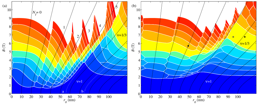
Figure 2: (Color online) (a) The ground state angular momentum phase diagram for a strong barrier ($\beta=1$) six-electron system as a function of the position of the potential barrier $r_{0}$ indicated by black lines, and the magnetic field $B$. The curvilinearity of the co-ordinate axis is due to the reason that when we move in the vertical direction in the phase diagram, $r_{0}$ in units of the oscillator length $l$ remains dimensionless constant as the magnetic field changes. The diagram separates into seven branches according to the number of electrons in the inner droplet $N_{I}$ indicated in the figure. (b) The same for a weak barrier ($\beta=0.2$). The color (lightness) indicates the angular momentum. For example, yellow (the lightest gray) corresponds to $M=45$, the angular momentum for filling fraction $\nu=1/3$ state found at large $r_{0}$.

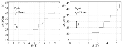
Figure 3: The ground state angular momentum along lines of constant $r_{0}$ in the $N_{I}=6$ branch of Fig. 2(a).

In both diagrams, the bottom phase corresponds to the minimum angular momentum of the maximum density droplet, in which the $N$ lowest angular momentum orbitals are compactly occupied. The wave function is the same as for the integer quantum Hall effect filling fraction $\nu=1$

z1z2⋯zN⋮⋮⋮⋮z1N−1z2N−1⋯zNN−1=𝒩​∏i<j(zi−zj)​e−∑i=1Nzi​z¯i/2,𝜓subscript𝑧1…subscript𝑧𝑁superscript𝑒superscriptsubscript𝑖1𝑁subscript𝑧𝑖subscript¯𝑧𝑖2⋅superscript𝜋𝑁12⋯𝑁fragments fragmentsz1fragmentsz2⋯fragmentsz𝑁⋮⋮⋮⋮fragmentsz1𝑁1fragmentsz2𝑁1⋯fragmentsz𝑁𝑁1𝒩subscriptproduct𝑖𝑗subscript𝑧𝑖subscript𝑧𝑗superscript𝑒superscriptsubscript𝑖1𝑁subscript𝑧𝑖subscript¯𝑧𝑖2\begin{split}\psi(z_{1},\ldots,z_{N})=&\frac{e^{-\sum_{i=1}^{N}z_{i}\bar{z}_{i}/2}}{\sqrt{\pi^{N}1!\cdot 2!\cdots N!}}\begin{tabular}[]{|cccc|}$1$&$1$&$\cdots$&$1$\\ $z_{1}$&$z_{2}$&$\cdots$&$z_{N}$\\ $\vdots$&$\vdots$&$\vdots$&$\vdots$\\ $z_{1}^{N-1}$&$z_{2}^{N-1}$&$\cdots$&$z_{N}^{N-1}$\\ \end{tabular}\\ =&\mathcal{N}\prod_{i<j}(z_{i}-z_{j})e^{-\sum_{i=1}^{N}z_{i}\bar{z}_{i}/2}\ ,\end{split}

11⋯111⋯1 (6)

with angular momentum $M=N(N-1)/2$.

At higher angular momenta above $\nu=1$, the potential barrier leads to the partition of the phase diagram according to the number of electrons $N_{I}=0,1,2,3,4,5,$ and $6$ in the inner electron droplet, or equivalently $N-N_{I}$ in the outer. At small $r_{0}$, when the $\delta$-function potential is close to the center of the external parabolic confinement potential, the density at the center vanishes and the electrons form a ring-like structure. When $r_{0}$ is increased by moving the potential barrier farther away from the origin, electrons tunnel into the quantum dot at the center of the system one by one. Finally, all electrons are in the dot, and the barrier only compresses the system giving rise to a reduced radius of the electron density by shifting the ground state transitions to higher magnetic fields and reorganizing the electron configuration. We start the detailed analysis of the phase diagrams from this regime.

We first analyse the system following lines a and b of Fig. 2(a). The corresponding angular momenta are shown in Fig. 3. As the magnetic field gets stronger, the successive phases tend to have angular momentum difference six (a) or five (b), as the electrons favour either a hexagonal configuration or a pentagonal configuration with one electron at the center.tolo Two exceptions are the small $M=35$ phase along line a and the $M=21$ phase along line b, which corresponds to a $\nu=1$ state with a hole at the center. The pentagonal phases have slightly larger radius than the corresponding phases that support hexagonal electron configurations so that the compression eventually favours the hexagonal configuation and counter-intuitively actually reduces the density near the center. A notable exception is the strong yellow (lightest gray) phase continuously connected to the Laughlin state at filling fraction $\nu=1/3$ with the wave function

$$\psi(z_{1},\ldots,z_{N})=\mathcal{N}\prod_{i<j}(z_{i}-z_{j})^{3}e^{-\sum_{i=1}^{N}z_{i}\bar{z}_{i}/2}\$$ (7)

and angular momentum $M=3N(N-1)/2$ that supports both the pentagonal and hexagonal electron configurations.

III.2 Weak coupling

Let us now analyze more carefully each branch in the weak coupling phase diagram. For this purpose, we define the angular momentum of the dot as $M_{D}=\sum_{m}n_{m}m$, where the sum is taken up to such $m$ that $\sum_{m}n_{m}=N_{I}$. If this orbital is shared between the ring and the dot, only the corresponding fraction of $n_{m}$ is employed in place of $n_{m}$. The angular momentum of the ring is then obtained from the total angular momentum as $M_{R}=M-M_{D}$. Note that in the coupled system $M_{R}$ and $M_{D}$ are in general not exact integers since the wave function typically contains superpositions of the two systems with different angular momenta summing to a given total angular momentum.

Figs. 4(a-f) show $M$ and $M_{R}$ as a function of $B$ along lines of constant $r_{0}$ chosen from branches $N_{I}=0$ to $N_{I}=5$ of the phase diagram. The corresponding occupation numbers for each ground-state angular momentum at the first magnetic field value on each plateau are listed in Figs. 4(g-l), where number of electrons in the dot $N_{I}$ run from $0$ to $5$.

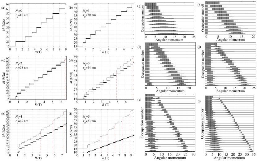
Figure 4: (Color online) The total ground state angular momentum (solid-line) and the angular momentum of the ring (black dots) along lines of constant $r_{0}$ in the $N_{I}=0,1,2,3,4$ and $5$ branches of Fig. 2(a). The vertical dashed red lines mark the transitions of the inner system. Occupation numbers for the ground states in panels (a-f) evaluated at the first magnetic field value at each plateau, the uppermost corresponding to $B=0$ T.

In Figs. 4(a) and (g) the angular momentum difference $\Delta M$ is always 6 indicating that the electrons form a hexagonal ring. Next in Figs. 4(b) and (h), $\Delta M=5$ and $M=M_{R}$ so that one electron occupies the $m=0$ orbital and the remaining five electrons are in the ring. Fig. 4(c) and (i) tell similar story, where now two first orbitals are occupied while the remaining 4 electrons are in the ring yielding $\Delta M=4$ and $M-M_{R}=1$. At about 6.5 T, there is a transition in the inner system as two electrons at the center excite to $m=1$ and $m=2$ giving $M-M_{R}=3$. In Fig. 4(d) and (j), there are two such transitions as $M-M_{R}$ is first 3, then it increases to 6 and finally to 9. In Figs. 4(e,k) and (f,l), we have similarly the frequent excitations of the ring with $\Delta M=2$ and $1$, respectively, and the less frequent excitations of the dot with $\Delta M=4$ and $5$, respectively. In the occupation numbers (Figs. 4(g-l)), these transition are seen such that subsequent states differ either by the inner or outer (or both) system moving one unit to the right.

We thus see that for $N_{I}<6$ the premier mechanism for gaining angular momentum is to periodically give the incremental angular momentum to the electrons of the exterior ring, which leads to the angular momentum difference $\Delta M=N-N_{I}$ for successive phases. The magnetic field range of each phase is then roughly a constant. The subsidiary mechanism is to increase the angular momentum of the inner system, which typically involves creation of a vortex near the center. In this case, the angular momentum shift is around $N$ depending on whether all or merely the inner electrons move radially outwards.

The transfer of electrons in and out of the quantum ring should be observable in the Aharonov-Bohm magnetic period.szafran We also expect the creation of vortices in the electron droplet to be observable in the conductivity in analogy with findings of Ref. muhle, for concentric quantum rings. In fact, by comparing the discs defined by the radius of density maximum in the quantum dot between the vertical dashed red lines in Fig. 4, we found that the area of the disc increased approximately by one in oscillator units at each transition, which in the limit $\omega_{0}\rightarrow 0$ corresponds to one magnetic flux quantum. Similar behaviour is observed for the area enclosed by the density maximum of the ring.

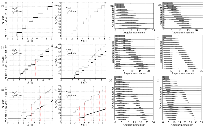
Figure 5: (Color online) The same as Fig. 5 for $\beta=0.2$.

The regular diamond structure in Fig. 2(a) is due to the symmetry blockade caused by the fact that the transfer of charge in and out of the droplet constitutes an immense change in the angular momentum as a large number of radially localized angular momentum orbitals fit in the space between the ring and the dot. We remark that the phases tend to get thinner in $r_{0}$ direction as we move to larger $r_{0}$ because the same amount of angular momentum orbitals become available for a smaller increase of $r_{0}$. This is due to the fact that the radial size of the orbital with quantum number $m$ is proportional to $\sqrt{m}$ rather than $m$.

The small phases near $r_{0}=0$, more visible for the weaker barrier in Fig. 2(b), are due to the fact that a normal parabolic quantum dot with six electrons supports the pentagonal electron configurations except at $M=21$ and $M=39$.tolo Since the influence of the potential is proportional to its perimeter, at sufficiently small $r_{0}$ the potential can no longer force the hexagonal configuration, and the ground-state angular momenta of a parabolic quantum dot, found also at the limit $r_{0}\rightarrow\infty$, are reacquired.

III.3 Strong coupling

Recall the ground state angular momentum phase diagram for $\beta=0.2$ shown in Fig. 2(b). As the strength of the barrier $\beta$ is weakened, the regular structure of the phase diagram present at a strong barrier strength is gradually lost as the coupling between the inner and outer system becomes larger and a more unilateral collective behaviour extends over the barrier. Due to scaling of the energies with the magnetic field as mentioned in Sec. II, the coherent structure fails first at weak magnetic fields.

Figs. 5(a-f) show $M$ and $M_{R}$ as a function of $B$ along lines of constant $r_{0}$ chosen from branches $N_{I}=0$ to $N_{I}=5$ of the phase diagram with the occupation numbers at each plateau listed in Figs. 5(g-l). Figs. 5(a,g) and (b,h) admit to the explanation of hexagonal and pentagonal electron configurations with 0 and 1 electron at the center as previously. At strong magnetic fields, Figs. 5(c-f) and (i-l) are reminiscent of the weak coupling case with excitations of the dot and the angular momentum of the ring increasing in definite steps. In the higher angular momentum states, the separation into two systems is evident in the occupation numbers. Main difference to the strong barrier case is the spreading of the angular momentum reflecting the strong coupling of the systems, best seen in Fig. 5(l). However, at weak magnetic fields the ring angular momentum is no longer constant suggesting that our simple picture breaks down due to the electron correlations. This is seen on the first few lines of the corresponding occupations in Figs. 5(j-l) where the electrons appear to be either in the dot or an excited dot.

In Fig. 5(i), the three small phases crossed by $r_{0}=40$ nm in Fig. 2(b) still have large weight on the two first orbitals corresponding to 2 electrons at the center and the quantity $N-\sum_{m=0}^{N-1}n_{m}$, where $n_{m}$ is the occupation of angular momentum orbital $m$, is exceedingly close to 1,2, and 3, respectively, demonstrating quantized charge depletion relative to the $\nu=1$ maximum density droplet. For the phases directly above $\nu=1$, the charge depletion is one electron charge to an accuracy of 1‰.

III.4 Edge green’s function

Even when all the electrons are inside the barrier, the compression still affects the edge details of the system. A quantity of interest for the tunnelling experiments that probe the chiral Luttinger liquid theory of the FQH edge in macroscopic samples is the current-voltage power-law dependence $I\propto V^{\alpha}$, and hence (in the thermodynamic limit) the power-law dependence of the edge Green’s function chang

$$G_{e}(z,z_{0})=\langle\psi^{\dagger}(z)\psi(z_{0})\rangle\ ,$$ (8)

which is called the edge Green’s function as it is evaluated along the edge. For an electron disc, we may set $z_{0}=r$ and $z=re^{i\theta}$, where $r$ is about the radius of the disc. According to the theory $|G_{e}|\propto|z-z_{0}|^{-\alpha}\propto|\sin(\theta/2)|^{-\alpha}$, where $\alpha$ reflects the topological order of the FQH phase. The experimental results are somewhat puzzling in that while there appears to be a clear non-Ohmic current-voltage power-law dependence $I\propto V^{\alpha}$ in accordance with the chiral Luttinger liquid theory of the FQH edge chang ; wen_adv , the exact value of the tunnelling exponent $\alpha$ appears to be sample dependent and in general notably less than the supposed universal value derived from the bulk effective theory. A number of mechanisms, including taking into account the long-range nature of the Coulomb interaction and edge reconstruction, whose effect amounts to renormalization of the power-law exponent $\alpha$, have been suggested by several authors chang . However, no clear consensus of the correct picture has been achieved so far.

For the $\nu=1/3$ phase, in which it is possible to continuously interpolate the superposition of the hexagonal and pentagonal electron configurations, the tunnelling exponent $\alpha$ decreases continuously as the compression is increased. This result is in agreement with the findings of Ref. wan, , where with a slightly different confinement potential and 8 electrons the exponent $\alpha$ was found to change after cutting the size of the single-particle basis. Fig. 6 illustrates the determination of the power-law exponent $\alpha$. The oscillations are seen to vanish as the edge is approached and the exponents $\alpha\approx 2.1$ and $2.8$ can be credibly extracted. However, this appears not to be the case for many of the phases below and above $\nu=1/3$ as well as other parts of the phase diagram where heavy oscillations of the edge Green’s function render the extraction of $\alpha$ rather uncertain (see Fig. 7). An exception is the $\nu=1$ phase, which has the power-law behaviour $\alpha=1$ typical of Fermi liquids.

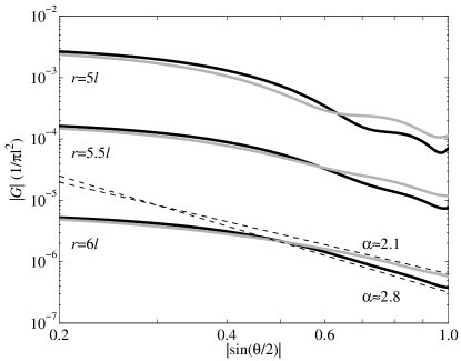
Figure 6: The edge Green’s functions at three radial distances $r$ for the two states in the $\nu=1/3$ topological phase marked by the squares in Fig. 2(b). The black square corresponds to the black line.

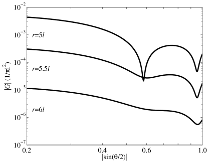
Figure 7: The edge Green’s function at three radial distances $r$ for at the point $r_{0}=30$ nm, $B=5.7$ T, and $\beta=0.2$ marked in the strong coupling phase diagram of Fig. 2(b).

IV Summary

We have studied cylindrically-symmetric electron droplet tunably coupled to a surrounding quantum ring in the strong magnetic field regime. The structure of the ground state angular momentum phase diagram was understood in terms of radial charge transfer, which should be observable in a lateral transport Aharonov-Bohm interferometer experiment. The compression induced by the potential barrier was also found to renormalize the tunnelling exponent of the edge Green’s function.

V Acknowledgements

This study has been supported by the Academy of Finland through its Centres of Excellence Program (2006-2011). ET acknowledges financial support from the Vilho, Yrjö, and Kalle Väisälä Foundation of the Finnish Academy of Science and Letters. We also thank C. Webb for useful discussions.

References

- (1) D. C. Tsui, H. L. Stormer, and A. C. Gossard, Phys. Rev. Lett. 48, 1559 (1982).
- (2) R. B. Laughlin, Phys. Rev. Lett. 50, 1395 (1983).
- (3) J. K. Jain, Phys. Rev. Lett. 63, 199 (1989).
- (4) X.-G. Wen, Adv. Phys. 44, 405 (1995).
- (5) C. Nayak, S. H. Simon, A. Stern, M. Freedman, and S. Das Sarma, Rev. Mod. Phys. 80, 1083 (2008).
- (6) H. Saarikoski and A. Harju, Phys. Rev. Lett. 94, 246803 (2005).
- (7) H. Saarikoski, E. Tölö, A. Harju, and E. Räsänen, Phys. Rev. B 78, 195321 (2008).
- (8) This corresponds to the lowest Landau level in the limit that the harmonic confinement potential of the quantum dot vanishes.
- (9) A. D. Güçlü, Q. F. Sun, H. Guo, and R. Harris, Phys. Rev. B 66, 195327 (2002).
- (10) B. Szafran, F. M. Peeters, and S. Bednarek, Phys. Rev. B 70, 125310 (2004).
- (11) A. Mühle, W. Wegscheider, and R. J. Haug, Appl. Phys. Lett. 91, 133116 (2007).
- (12) M. Büttiker and C. A. Stafford, Phys. Rev. Lett. 76, 495 (1996).
- (13) T. Ihn, M. Sigrist, K. Ensslin, W. Wegscheider, and M. Reinwald, New J. Phys. 9, 111 (2007).
- (14) A. Fuhrer, P. Brusheim, T. Ihn, M. Sigrist, K. Ensslin, W. Wegscheider, and M. Bichler, Phys. Rev. B 73, 205326 (2006).
- (15) E. Tölö and A. Harju, Phys. Rev. B 79, 075301 (2009).
- (16) The Landau-level mixing shifts the transitions to higher magnetic fields, see for example S. Siljamäki, A. Harju, R. M. Nieminen, V. A. Sverdlov, and P. Hyvönen, Phys. Rev. B. 65, 121306(R) (2002).
- (17) E. V. Tsiper, J. Math. Phys. (N.Y.) 43, 1664 (2002).
- (18) A. M. Chang, Rev. Mod. Phys 75, 1449 (2003).
- (19) X. Wan, F. Evers, and E. H. Rezayi, Phys. Rev. Lett. 94, 166804 (2005).