The initial mass function of the rich young cluster NGC 1818 in the Large Magellanic Cloud

Abstract

We use deep Hubble Space Telescope photometry of the rich, young ($\sim$20–45 Myr-old) star cluster NGC 1818 in the Large Magellanic Cloud to derive its stellar mass function (MF) down to $\sim 0.15$ M_⊙. This represents the deepest robust MF thus far obtained for a stellar system in an extragalactic, low-metallicity ([Fe/H] $\simeq-0.4$ dex) environment. Combining our results with the published MF for masses above 1.0 M_⊙, we obtain a complete present-day MF. This is a good representation of the cluster’s initial MF (IMF), particularly at low masses, because our observations are centred on the cluster’s uncrowded half-mass radius. Therefore, stellar and dynamical evolution of the cluster will not have affected the low-mass stars significantly. The NGC 1818 IMF is well described by both a lognormal and a broken power-law distribution with slopes of $\Gamma=0.46\pm 0.10$ and $\Gamma\simeq-1.35$ (Salpeter-like) for masses in the range from 0.15 to 0.8 M_⊙ and greater than 0.8 M_⊙, respectively. Within the uncertainties, the NGC 1818 IMF is fully consistent with both the Kroupa solar-neighbourhood and the Chabrier lognormal mass distributions.

1 Introduction

The shape of the stellar initial mass function (IMF) is of great importance in modern astrophysics. It plays a crucial role in many of the remaining ‘big’ questions, e.g., the formation and evolution of the first stars and galaxies. Whether or not the IMF is universal remains hotly contested (e.g., Scalo 1998, 2005; Eisenhauer 2001; Gilmore 2001; Kroupa 2007; and references therein). Obtaining the IMF is challenging because stellar masses cannot be measured directly, while limitations due to the observational technology used affect accurate analysis of, particularly, the low-mass stars.

Star clusters, both open and globular clusters, represent ideal objects to address many astronomical problems because all of their member stars have the same age and metallicity and are located roughly at the same distance. Much work has been done on the MFs of globular clusters (GCs) in the Milky Way. Paresce et al. (2000) found that the MFs of Galactic GCs are best approximated by a lognormal function, based on their analysis of the MFs of a dozen Galactic GCs for stellar masses below 1 M_⊙. However, since all Galactic GCs are old ($t\ga 10$ Gyr, with typical relaxation times of $\sim 0.1$ Gyr), they can only provide evolutionary information on a single (long) time-scale; stellar and dynamical evolution must obviously have affected the MF at high masses (e.g., de Grijs et al. 2002a,b). The Large Magellanic Cloud (LMC), on the other hand, is a unique laboratory for studying star cluster evolution on a range of time-scales as it contains a large population of rich star clusters with masses similar to those of Galactic GCs and covering ages from 0.001 to 10 Gyr (e.g., Beaulieu et al. 1999; Elson et al. 1999), thus making it possible to study clusters at (almost) all evolutionary stages. Particularly for the rich, young clusters, stellar and dynamical evolution have not yet affected the MF at low masses, so we can attempt to obtain the low-mass IMF of these young clusters from their present-day mass functions (PDMFs). The unprecedented high spatial resolution of the Hubble Space Telescope (HST) allows us to resolve individual stars in dense star clusters at the distance of the LMC, $\sim$50 kpc.

Table 1: Fundamental parameters of NGC 1818.

		Ref.
RA, Dec (J2000)	$05^{\rm h}04^{\rm m}03^{\rm s}$, $-66^{\circ}26^{\prime}00^{\prime\prime}$	1
$M_{V}$ (mag)	$-8.8$	4,6
log(Age yr-1)	$7.65\pm 0.05$	2a
	$7.25\pm 0.40$	2b
[Fe/H] (dex)	$\sim-0.4$	4
$E(B-V)$ (mag)	0.03	3
$(m-M)_{0}$ (mag)	18.58	3
Mass (M⊙)	$2.8\times 10^{4}$	5
$R_{\rm core}$ (pc)	2.1 $\pm$ 0.4	7
$R_{\rm hl}$ (pc)	2.6	8

NGC 1818 is a young, compact cluster (see Table 1 for the cluster’s fundamental parameters). It has been studied extensively (e.g., Will et al. 1995; Elson et al. 1998; Johnson et al. 2001; de Grijs et al. 2002a,b,c). Will et al. (1995) studied the cluster’s IMF using the ESO/MPIA 2.2m telescope at La Silla observatory, Chile, but only for the massive stars ($V\leqslant 22.75$ mag, corresponding to masses $\ga 1.26$ M_⊙). de Grijs et al. (2002a,b) obtained the MF above 1 M_⊙ using (in part) the same data as analysed in this paper and concluded that the cluster’s MF is largely similar to the Salpeter (1955) IMF approximation over this mass range. The cluster’s IMF for stellar masses below 1 M_⊙ is still unknown.

Given the young age of NGC 1818, most of its member stars with masses below 1.0 M_⊙ are still on the pre-main sequence (PMS). Although PMS membership-selection criteria have been established for the separation of PMS stars from low-mass (zero-age) main-sequence objects (Park et al. 2000; Sung et al. 2000), using PMS stars is very challenging on the basis of optical observations alone because these stars are usually very faint overall and therefore difficult to detect with most ground-based instruments. The stellar systems in the LMC are thought to be the best places to search for PMS stars because they do not suffer from either severe crowding or significant extinction (Gouliermis et al. 2006a). The evolution of PMS stars is still rather uncertain (e.g., Baraffe et al. 1998), which implies that the choice of one’s input parameters will significantly affect the predicted PMS evolution. White et al. (1999) compared six PMS evolution models and concluded that the models of Baraffe et al. (1998) resulted in the most consistent ages and masses (Park et al. 2000). On the basis of the best available evolutionary models (Baraffe et al. 1998), in this paper we obtain the low-mass IMF (below 1.0 M_⊙) for the young LMC cluster NGC 1818 based on high-resolution HST data.

Although new evolutionary models for young low-mass stars have appeared in the literature (see for a review Hillenbrand & White 2004) since the comparative analysis of White et al. (1999), we emphasise that the models of Baraffe et al. (1998) use the most up-to-date equation of state (which was validated on the basis of high-pressure experiments) and outer-boundary conditions based on non-grey atmosphere models (see for details Chabrier et al. 2005; Mathieu et al. 2007). More recent models either use an equation of state that is more appropriate for solar-type and more massive stars, but not for the interior conditions of low-mass stars (cf. Yi et al. 2003; Dotter et al. 2008), or approximate grey outer-boundary conditions which provide incorrect effective temperatures and luminosities in the presence of molecules (Palla & Stahler 1999). The Dotter et al. (2008) models use the same atmosphere models (Hauschildt et al. 1999) as Baraffe et al. (1998) while the Siess et al. (2000) models use similar input physics and are very comparable in the low-mass stellar domain. Finally, the Chabrier et al. (2000) models are most suitable for ‘dusty’ conditions, i.e., for objects with lower masses than discussed here. The Baraffe et al. (1998) models have been extensively validated observationally for objects of different ages and masses below 1 M_⊙, using different observational constraints (such as mass-radius and mass-luminosity relationships, colour-magnitude diagrams, spectra and binary systems). The only model suite comparable in terms of input physics and quality are the Siess et al. (2000) models. However, they do not include metallicities below $Z=0.01$.

In Section 2 we present the observations and data-reduction steps in detail. We describe how we obtain the cluster’s low-mass IMF in Section 3. Finally, we discuss our results and provide a summary in Sections 4 and 5.

2 Observations and data reduction

2.1 Observations

As part of HST programme GO-7307, we have a unique set of high-quality imaging observations of NGC 1818, obtained with both the Wide-Field and Planetary Camera-2 (WFPC2) and the Space Telescope Imaging Spectrograph (STIS). The cluster was part of a carefully selected LMC cluster sample (see Beaulieu et al. 1999). It has an age of $\approx 45$ Myr and a mass of $\approx 10^{4}$ M_⊙ (see Hunter et al. 1997; Beaulieu et al. 1999; de Grijs et al. 2002a). WFPC2 is composed of four chips (each containing 800$\times$800 pixels), one Planetary Camera (PC) and three Wide-Field (WF) arrays. The PC’s field of view is about 34$\times$34 arcsec² (with a pixel size of 0.0455 arcsec) and the field of view of each of the WF chips is about 150$\times$150 arcsec² (with a pixel size of 0.097 arcsec). The STIS field of view is 28$\times$52 arcsec², with a pixel size of 0.0507 arcsec.

We obtained WFPC2 exposures through the F555W and F814W filters (roughly corresponding to the Johnson-Cousins $V$ and $I$ bands, respectively), with the PC centred on both the cluster core and its half-mass radius. We have both deep (exposure times of 140 and 300 s for each individual image in F555W and F814W, respectively) and shallow (exposure times of 5 and 20 s, respectively) images with the PC located on the cluster centre (Santiago et al. 2001; de Grijs et al. 2002a). For the exposures centred on the cluster’s half-mass radius we obtained deep observations with a total exposure time of 2500 s in both filters.

Given that NGC 1818 is observed superimposed on the LMC background field, it is important to (statistically) subtract the background stars to obtain clean luminosity and mass functions. We obtained very deep WFPC2 exposures through the F555W and F814W filters from the HST Data Archive of the general LMC background and of a specific background region associated with NGC 1818 (see, for more details, Castro et al. 2001; Santiago et al. 2001; de Grijs et al. 2002a). For the general background the exposure times were 7800 s (F555W) and 5200 s (F814W) (de Grijs et al. 2002a), while they were 1200 s (F555W) and 800 s (F814W) for the images of the specific background field associated with the cluster (Santiago et al. 2001; de Grijs et al. 2002a). Both sets of background fields were significantly deeper than the targeted cluster observations, hence allowing us to properly correct for background effects at the faintest magnitudes covered by our science observations.

We also obtained deep STIS CCD observations in ACCUM imaging mode through the F28$\times$50LP long-pass filter (central wavelength $\lambda_{\rm c}=7230$Å), with the CCD centred on the half-mass radius of NGC 1818. The total exposure time of this observation was 2950 s in a set of 5 observations (see also Elson et al. 1999); each observation was split into two exposures to allow for the removal of cosmic rays by the data-processing pipeline. The deep STIS data allow for the construction of very deep luminosity functions; in fact, STIS (in imaging mode through long-pass filters) is five times more sensitive for faint red objects than WFPC2 (e.g., de Grijs et al. 2002a).

2.2 Data reduction and photometry

We used the iraf/APPHOT package to perform aperture photometry. We compared the different colour-magnitude diagrams (CMDs) for 1-, 2-, 3- and 4-pixel apertures and found that the 2-pixel aperture was best suited for stellar aperture photometry in this cluster since it produced the smallest photometric errors and the tightest main sequence. This radius corresponds to $\sim$0.09 arcsec for the PC chip, $\sim$0.2 arcsec for the WF chips and $\sim$0.1 arcsec for STIS. It is a compromise between the need to include the core of the point-spread function (PSF) but avoid contamination from nearby objects (cf. de Grijs et al. 2002a).

We emphasise that point-spread function (PSF) fitting and aperture photometry are both suitable techniques one can use in the type of environment we are dealing with here. There are pros and cons associated with either method. Here, we have followed established practice for NGC 1818 (and our other sample clusters; cf. de Grijs et al. 2002a,b,c) based on HST observations (see Castro et al. 2001; Santiago et al. 2001; Beaulieu et al. 2001; Johnson et al. 2001; de Grijs et al. 2002a,b,c; Hu et al. 2009), for which we showed that the resulting data quality based on aperture photometry is robust and sufficient. The key issues are that (i) the sky background should be as constant as possible (which is met because of the high-quality HST observations available), (ii) we have carefully determined aperture corrections based on TinyTim simulated PSF analysis (Krist & Hook 2001), and (iii) our error bars reflect the approach used; we base our results on a proper and careful analysis of the observed signal in terms of the error bars. The latter is most crucial and was carefully implemented in our modeling. The photometric uncertainties of the vast majority of our individual STIS magnitudes are less than 0.05 to 0.10 mag, while none of the stars in our final sample have uncertainties greater than 0.20 mag.

We adopted the relations of Whitmore et al. (1999) to correct the resulting photometry for the effects of charge-transfer (in)efficiency (CTE):

$$Y\mbox{-CTE} = 2.3\times 10^{-0.256\times\log({\it BKG})}$$ (1)

$$\times[1+0.245\times(0.0313-0.0087\log{\it CTS}_{\rm obs})$$

$$\times({\rm MJD}-49471)];$$

$$X\mbox{-CTE} = 2.5$$ (2)

$$\times[1+0.341\times(0.00720-0.0020\log{\it CTS}_{\rm obs})$$

$$\times({\rm MJD}-49471)].$$

The total CTE correction is obtained as

$${\it CTS}_{\rm cor} = (1+\frac{Y\mbox{-CTE}}{100}\times\frac{Y}{800}+\frac{X\mbox{-CTE}}{100}\times\frac{X}{800})\times$$ (3)

$${\it CTS}_{\rm obs},$$

where CTS_cor is the number of counts after CTE correction, CTS_obs is the raw number of counts, $Y$-CTE is the CTE loss (in per cent) over 800 pixels in the $Y$ direction and $X$-CTE is the equivalent factor in the $X$ direction, $X$ and $Y$ are the $x$ and $y$ positions of the star in pixels, BKG is the mean number of counts for a blank region of the background field and MJD is the modified Julian date.

Before applying aperture corrections (ACs), we also used iraf/stsdas to correct for the geometric distortion of the WFPC2 chips. We determined the ACs for our photometry based on the model PSFs generated by TinyTim (Krist & Hook 2001). We used single ACs for the entire chip, because if we change the position where we generate the TinyTim PSF image the ACs are very similar (positional differences in the ACs are less than 0.02 mag across the detector). We first constructed artificial TinyTim PSF images for each passband and each chip. Next, we measured the flux within a 2-pixel circular aperture and compared this with the total flux in the artificial PSF, thus giving us the AC for any given filter/chip combination (listed in Table 2). We used the same photometric method for the STIS F28$\times$50LP image.

Table 2: Aperture corrections.

Filter	Chip	AC (mag)
F555W	PC	0.424
	WF2	0.258
	WF3	0.307
	WF4	0.274
F814W	PC	0.607
	WF2	0.282
	WF3	0.334
	WF4	0.298
F28$\times$50LP	STIS	0.506

We adopted the method of Holtzman et al. (1995) to convert the aperture-corrected WFPC2 photometry to the standard Johnson-Cousins $V$ and $I$ passbands:

$$V = -2.5\times\log\dot{C}({\rm F555W})+(-0.052\pm 0.007)\times(V-I)$$ (4)

$$+(0.027\pm 0.002)\times(V-I)^{2}+(21.725\pm 0.005)$$

$$+2.5\times\log(GR)$$

and

$$I = -2.5\times\log\dot{C}({\rm F814W})+(-0.062\pm 0.009)\times(V-I)$$ (5)

$$+(0.025\pm 0.002)\times(V-I)^{2}+(20.839\pm 0.006)$$

$$+2.5\times\log(GR),$$

where $\dot{C}$ is the count rate in 2-pixel apertures and $GR=1.987,2.003,2.006$ and 1.955 for the PC, WF2, WF3 and WF4 chips, respectively (Holtzman et al. 1995).

Figure 1 shows the CMD of NGC 1818 based on our WFPC2 data. Figure 2 represents the spatial distribution of the stars in the NGC 1818 field as observed with WFPC2 and STIS (dots and solid rectangular area, respectively).

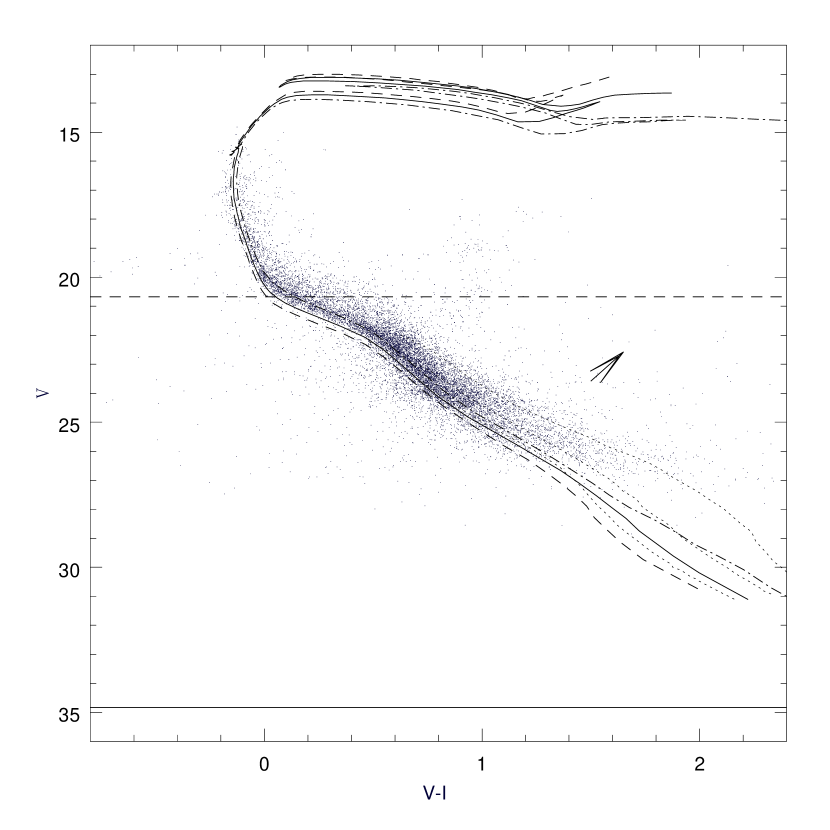
Figure 1: HST/WFPC2 CMD of NGC 1818. The photometry was converted to the standard $V$- and $I$-band filters using Eqs. (4) and (5). From bottom to top (in the direction of the arrow) the three dotted lines represent isochrones (Baraffe et al. 1998) of log(Age yr^-1) = 7.25 (best fit to the average PMS) and metallicities $Z=0.0019,0.006$ and 0.019, respectively. The dashed, solid and dot-dashed lines represent Padova isochrones (Girardi et al. 2000) of log(Age yr^-1) = 7.65 (best fit to the main sequence) and metallicities $Z=0.004,0.008$ and 0.019, respectively. The horizontal dashed and solid lines represent, respectively, the upper and lower magnitude limits to the colour-magnitude space covered by our STIS observations.

Figure 2: Spatial distribution of the stars in NGC 1818. The dots represent the stars detected in the WFPC2 observations. The solid rectangular area indicates the area covered by our STIS observations and the short-dashed square delineates the area used for further analysis in this paper (see Section 3.3).

2.3 Completeness

Because of the cluster’s stellar density gradient, one of the most difficult problems for MF derivation involves completeness correction, which is normally a function of position within a cluster. We used a similar method of completeness correction as de Grijs et al. (2002a). They computed the corrections in circular annuli around the cluster centre. However, we simply computed the equivalent corrections for the entire chip for the exposures centred on the cluster’s half-mass radius, as well as for the entire STIS chip, because both sets of observations are centred on roughly the same position and the area around the half-mass radius is not as crowded as the cluster centre. The effects of sampling incompleteness are constant across our STIS field, within the observational uncertainties (see also de Grijs et al. 2002a). The same method was used for the completeness corrections applied to the background field, although for the magnitude range of interest the completeness of the background field is close to unity.

Figure 3: Completeness curves for NGC 1818. (Top) Solid line: STIS; dotted line: PC (F555W); short-dashed line: PC (F814W). The horizonal dashed line represents the 50 per cent completeness limit. (Bottom) Radially-dependent completeness curves of the STIS observations.

We added an area-dependent number of artificial sources of Gaussian shape to each chip for input magnitudes between 15.0 and 30.0 mag, in steps of 0.5 mag. We then applied the same photometric method to the fields including both the cluster stars and the artificial sources, to quantitatively assess how many artificial stars we can detect after correction for chance blends and superpositions. Figure 3 shows the completeness curves of the STIS and PC chips. The bottom panel shows that the STIS completeness curves are not significantly radially dependent. We therefore used the completeness corrections for the STIS data as a whole (the variation of the different curves near the 50 per cent completeness limit is negligible in relation to the observational uncertainties). The results shown have all been corrected for blending of multiple randomly placed artificial stars and for superposition of artificial and real stars in the cluster region. For our analysis in the remainder of this paper we only consider magnitude ranges that are $\geq 50$ per cent complete.

3 Analysis

3.1 Evolutionary model, age and metallicity

Since the observations were obtained in two WFPC2 and one STIS filter, we obtain three LFs, in the F555W, F814W and F28$\times$50LP bands. These must be converted to a common parameter (e.g., mass) for comparison purposes. de Grijs et al. (2002b) studied the MF of NGC 1818, based on the WFPC2 data, and adopted three mass-luminosity (ML) conversions for stellar masses above $\sim$1.0 M_⊙, for solar and subsolar metallicities and a cluster age of 25 Myr. We can reach much lower masses using the STIS data because of the much longer exposure times employed. All of the stars detected by STIS are faint and (hence) of low mass (assuming that they are cluster members), as is apparent from a direct comparison of the stars in common on the shallower WFPC2 exposures and the deep STIS frames centred on the cluster’s half-mass radius. For the young age of the cluster this implies that most of these objects are likely PMS stars. For the stars in common with the WFPC2 observations (the brighter stars detected on the STIS frames), this is supported by their loci in the CMD, because many stars are located above the zero-age main sequence (ZAMS) of NGC 1818, at least for low masses and on the basis of WFPC2 photometry alone (see Fig. 1). This distribution of the photometric data points is not due to biases caused by photometric uncertainties.

White et al. (1999) concluded that the models of Baraffe et al. (1998) result in the most consistent age and mass estimates, on the basis of a detailed comparison of six PMS evolutionary models. We therefore adopted the Baraffe et al. (1998) models for low-mass (PMS and ZAMS) stars and recalculated the models for the specific filters used in this paper and for a more extended range of metallicities and higher stellar masses (up to 1.4 M_⊙). Although a comparison of the Baraffe et al. (1998) PMS and the Girardi et al. (2000) main sequence models with our observational CMD appears to imply that up to 88 per cent of the stars detected by STIS ($\sim\in$ [22.6,27.8] mag) may be PMS stars, it is difficult to ascertain whether or not a given star is on the PMS, so the full, extended mass coverage of the Baraffe et al. (1998) models significantly aids in the interpretation of our results. In addition, we added photometry in the F28$\times$50LP filter to the model calculations.

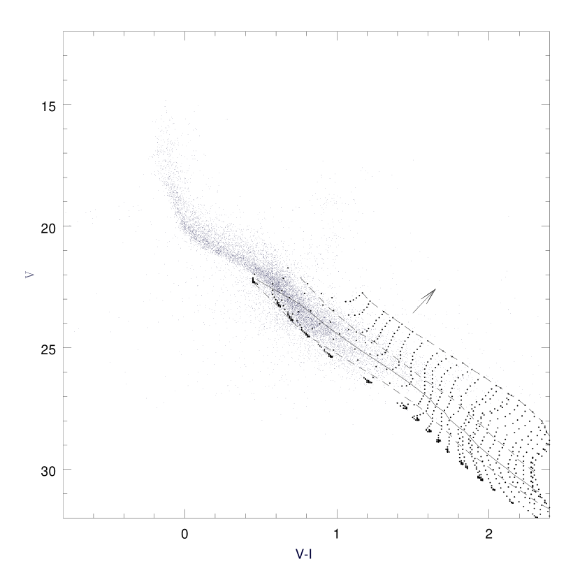
Figure 4: Baraffe et al. (1998) models with $Z$= 0.006 overlaid on the cluster’s CMD. The dotted lines are the PMS evolutionary tracks. The three dashed lines represent isochrones of log(Age yr^-1) = 7.65, 6.85 and 6.0, respectively (in the direction of the arrow). The solid line represents an isochrone of log(Age yr^-1) = 7.25, which traces the most appropriate average age for the PMS stars in the cluster.

Although we cannot use CMD analysis to attack the PMS uncertainties for the bulk of the STIS data, we know that the area observed by STIS overlaps with the WFPC2 observations centred on the cluster’s half-mass radius. Many (more than 1000 after completeness correction) of the faint stars in the STIS image are also detected in our WFPC2 observations and most of the stars in common between the two catalogues are PMS stars. As clearly shown in Fig. 4, the PMS stars observed by WFPC2 seem to exhibit a scatter in age (e.g., compare the youngest and oldest PMS isochrones in Fig. 4 with the data points).

To derive the age of PMS stars, it is common practice to compare their loci on the CMD with respect to the ZAMS (e.g., Park et al. 2000; Gouliermis et al. 2006a). This can be done for the brighter stars in the STIS field of view using the WFPC2 observations in common. Using the CMD of the low-mass stars observed with WFPC2 (Fig. 4), we realized that the PMS stars are distributed in a rather narrow region (see the detailed discussion below) and that most stars are located parallel to the main sequence (Park et al. 2000). Therefore, we can assume that all low-mass PMS stars detected by STIS have a mean age (and spread) centred on the ‘PMS sequence’, so that a MF for the PMS stars can be derived. Older and younger age sequences spanning the full CMD loci of the PMS stars detected in the WFPC2 data are used to measure the uncertainties associated with using this method. This way, the MF derived from the low-mass end of the WFPC2 data can be extended to the much deeper STIS photometry, by adopting a well-justified mean age (and uncertainty) and thus a specific ML conversion. This will allow us to probe well into the subsolar-mass regime at a hitherto unexplored (subsolar) metallicity.

We adopted the Padova isochrones (Girardi et al. 2000) to fit the main-sequence ridge line in the CMD and the Baraffe et al. (1998) evolutionary models to fit the PMS loci. In the direction of the arrow in Fig. 1, the dashed, solid and dot-dashed lines represent the best Padova isochrone fits for metallicities, $Z=0.004,0.008$ and 0.019 (Z_⊙), for log(Age yr^-1) = 7.65 ($\simeq 45$ Myr). The $Z=0.008$ isochrone provides the best fit to the main sequence of NGC 1818. However, the Baraffe et al. (1998) model suite does not include this metallicity, so we compare their models of $Z=0.0019,0.006$ and 0.019 (dotted lines in Fig. 1, from bottom to top in the direction indicated by the arrow). The difference between the models with $Z=0.006$ (Baraffe et al. 1998) and 0.008 (Girardi et al. 2000) is negligible, so we will use the Baraffe et al. (1998) $Z=0.006$ model for our PMS analysis. The dotted lines in Fig. 4 are the corresponding evolutionary tracks for low-mass stars with $Z=0.006$. In the direction of the arrow in Fig 4, the dashed lines represent isochrones of $Z=0.006$ and log(Age yr^-1) = 7.65, 6.85 and 6.0. Any stars located above the middle dashed line are most likely affected by significant photometric scatter (note that the effects of binary stars are small compared to the observed width of the CMD; cf. Hu et al. 2009). We therefore determine the mass of the low-mass stars based on the adopted model of log(Age yr^-1) = 7.25 (solid line in Fig. 4) as it represents the average age of the best-fitting isochrones.

3.2 Background subtraction

As already discussed by Castro et al. (2001), an old red-giant population and an intermediate-age red-clump population are clearly seen in the CMD of NGC 1818. These older components can only be interpreted as field stars in the LMC’s disc. To get a clean MF, the field-star contamination must be subtracted. There are two relevant sets of background observations obtained with WFPC2 available in the HST Data Archive, a background field associated with the cluster itself and a general LMC field. We decided to use the general field because it provides deeper photometry than the background associated with the cluster. (The 50 per cent completeness limit for the general LMC field was determined at $m_{\rm F555W}\simeq 27.5$ mag, while the equivalent limit for the field associated with the cluster occurs at $m_{\rm F555W}\simeq 26.3$ mag.)

Castro et al. (2001) adopted isochrones of old age to fit the background population (see their fig. 5), which implies that the NGC 1818 main sequence is severely contaminated by the low-mass main-sequence field stars. It is therefore of the utmost importance to carefully subtract this contaminating population. In addition, the stars detected in the general background field are all of low mass. Because of the very long exposure time of the general background field (7800 and 5200 s in F555W and F814W, respectively), all high-mass stars are saturated. The mass distribution in the field is therefore obviously different from the cluster MF (cf. the solid curve in Fig. 5) and must be subtracted carefully (and in a statistical sense) from the cluster MFs.

Figure 5: Mass distribution adopting Baraffe et al. (1998) ML relations for different ages in the common WFPC2/STIS area (after background subtraction); the solid curve shows the mass distribution of the general background.

We do not have access to a background field in the STIS F28$\times$50LP passband. Instead, we use the F814W photometry as a proxy for the general background in the STIS field of view because its effective wavelength is closest to the central wavelength of the F28$\times$50LP band. Even so, the observations of the general background are still not as deep as the STIS data. Gouliermis et al. (2006b) suggested that the stellar mass distribution in the field of the LMC follows a broken power-law distribution, based on their study of the general background field of LMC’s inner disc. In addition, the stellar mass function below 1.0 M_⊙ is generally considered to be well approximated by both a broken power-law (e.g., Kroupa 2001; Kroupa et al. 2003; Covey et al. 2008) and a lognormal distribution (e.g., Paresce et al. 2000; Chabrier 2003; Andersen et al. 2008; Hennebelle & Chabrier 2008). Therefore, we adopted both a power-law (with a slope $\Gamma$=1.87$\pm$0.06, where the IMF, $\xi$(m) $\propto$ $m^{\Gamma}$) and a lognormal function to approximate and extrapolate the general-background MF for masses between 0.15 and 0.63 M_⊙, the mass range where we only have STIS photometry.

3.3 The mass function

For WFPC2 we focus on the observations centred on the cluster’s half-mass radius, because they are much deeper (hence reaching lower masses) than the pointings centred on the cluster core, and well outside the most crowded region. As WFPC2 covers a much larger field of view than STIS, we must carefully choose the area in common for a proper comparison of the different MFs. We used the dashed square region shown in Fig. 2 for this purpose, for which we calculated the low-mass MFs in NGC 1818 based on both the high-resolution PC data and the STIS field of view. The MF from the common area on STIS is identical to that from the full STIS field of view and thus the mass distribution of the common area is fully representative of the cluster’s MF as a whole at this distance from the cluster centre.

Figure 6: Mass-luminosity relations for different ages based on the Baraffe et al. (1998) models.

We assume that all low-mass stars observed with STIS have the same age (see Sect. 3.1). The most likely age range for the entire stellar population runs from log(Age yr^-1) = 6.85 to 7.65. The models for different ages are characterized by different ML relations (see Fig. 6). Adopting different models for our luminosity-to-mass conversion will therefore lead to variations in the mass distribution, including in the mass range and the number of stars in each mass interval (see Fig. 5).

Figure 7: Complete MF of NGC 1818, based on background subtraction assuming a power-law IMF at low masses. Open squares: high-mass MF (de Grijs et al. 2002b); solid squares: STIS MF (this paper); triangles: WFPC2 MF (this paper). The dashed lines represent the standard Kroupa (2001) IMF.

Figure 8: Complete MF of NGC 1818, based on background subtraction assuming a lognormal IMF at low masses. The symbol coding is as in Fig. 7. The dashed lines show the standard Kroupa (2001) IMF while the solid line represents the best-fitting lognormal distribution.

The WFPC2 F814W filter has a central wavelength ($\lambda_{\rm c}=8012$Å) which is much closer to that of the STIS F28$\times$50LP passband ($\lambda_{\rm c}=7230$Å) than the WFPC2 F555W filter ($\lambda_{\rm c}=5439$Å). The number of stars detected in the F814W observations is closer to that found in the F28$\times$50LP frames than the stellar numbers in the F555W observations. Figures 7 and 8 show the mass distributions obtained on the basis of the observations in the two filters (F814W and F28$\times$50LP for the WFPC2 and STIS data, respectively) in the common area. The difference between both figures relates to the assumption adopted regarding the shape of the low-mass IMF for background subtraction: in Fig. 7 we assumed a power-law IMF, while in Fig. 8 a lognormal distribution was imposed. The solid squares are based on the STIS data and the triangles originate from the PC. For masses below 0.8 M_⊙, the STIS observations yield more low-mass stars than WFPC2. This may reflect the true mass distribution of the low-mass stars in NGC 1818. For stellar masses greater than 0.8 M_⊙ we use the results from the WFPC2 observations, since the STIS images are saturated at these bright magnitudes. At $\log({\rm Mass}/{\rm M}_{\odot})=-0.1$ and 0.0, where stars were detected on both the WFPC2 and STIS chips, we found 1153 stars in common between the two instruments (see Figs. 7 and 8). All WFPC2 stars used to derive the mass function at high masses are main-sequence stars, while of the STIS-detected stars below 0.8 M_⊙, $\sim 2226$ are PMS candidates (see for details Table 3). We combined the mass distribution from the two sets of observations to construct a clean MF spanning the full range from 0.15 to 1.25 M_⊙, as shown in Figs. 7 and 8.

4 Discussion

de Grijs et al. (2002b) studied the PDMF of NGC 1818 for masses above $\sim$1 M_⊙ based on three ML relations. The results from the different ML relations appear similar, with a PDMF slope closely approximated by the Salpeter (1955) IMF slope ($\Gamma=-1.35$) for the cluster as a whole. In this paper, we cover a mass interval in common with their results, so that we can construct a complete, combined MF for NGC 1818. We adopt the results from de Grijs et al. (2002b) based on the Kroupa, Tout & Gilmore (1993) ML relation (because this IMF extends to the highest stellar masses in NGC 1818) and combine their MF with our own determination of the PDMF for lower masses to obtain a complete MF for stellar masses above 0.15 M_⊙ (Figs. 7 and 8).

The usual method to derive the ages and masses of PMS stars is based on their loci in the CMD (Gouliermis et al. 2006a; Park et al. 2000). Although this approach is not possible for our STIS observations, we can use a priori information to help us constrain the most likely age range. Park et al. (2000) analysed the PMS stars in the young cluster NGC 2264 and found that most were distributed along a sequence parallel to the main sequence. We can use this information to justify our assumption that all PMS stars detected by STIS have the same age, which we obtain by fitting the Baraffe et al. (1998) evolutionary models to the observed sequence.

Figure 9: NGC 1818 MF based on ML relations for different ages.

We already concluded that – based on the WFPC2 observations – the most likely age range spanned by the PMS stars in NGC 1818 covers the interval from log(Age yr^-1) = 6.85 to 7.65. This, combined with the symmetrical spread of the data points between these age boundaries, leads us to adopt a mean age for the NGC 1818 PMS stars of log(Age yr^-1) = 7.25. The resulting MF for the youngest age constraint, combining the STIS and PC data, is shown in the left-hand panel of Fig. 9 and tabulated in Table 3; the right-hand panel shows the equivalent MF for the oldest age constraint. For the youngest age constraint, the best fit to the power-law slope of the MF gives $\Gamma=0.20\pm 0.08$. On the other hand, for log(Age yr^-1) = 7.65, $\Gamma=0.43\pm 0.16$.

Table 3: NGC 1818 mass function.

$\log(m_{\ast}/{\rm M}_{\odot}$)	$N$	$\log(m_{\ast}/{\rm M}_{\odot}$)	$N$
$-$0.80	525	0.36	83
$-$0.70	497	0.44	54
$-$0.60	566	0.52	48
$-$0.35	638	0.60	23
$-$0.10	1099	0.68	25
0.00	399	0.76	29
0.04	350	0.84	23
0.12	252	0.92	18
0.20	240	1.00	15
0.28	80

Our results rely on the assumption that the cluster’s mass function consists of single stars. This seems a reasonable assumption because the effect of unresolved binarity is expected to be very small. Kerber & Santiago (2006) analysed the effect of binaries on MFs containing different binary fractions and characterised by different MF slopes with $\alpha$ down to 0.8. Our slope corresponds to $\alpha$=0.54. The binary fraction at these low masses is poorly known. Marchal et al.(2003) and Delfosse et al. (2004) obtained a binary fraction of about 30 per cent for this low-mass range. L. Kerber (priv. comm.) kindly recomputed the tests done in Kerber & Santiago (2006) and added a binary fraction of 30 per cent, with $\alpha$ down to 0.4. The resulting MF (which is, strictly speaking, a system MF and not a single-star MF) characterised by a binary fraction of 30 per cent is identical to one with no binarity over the entire stellar mass range of interest, within the uncertainties associated with our results, so that we conclude that binarity does not play a crucial role in our results, for neither random pairing nor constant mass-ratio binaries. (Clearly, binaries will affect the final mass function, but the effect is expected to be small or negligible in relation to the uncertainties. Hu et al. [2009] derived $\sim$60 per cent binarity for NGC 1818 for the more massive F-type stars.)

We used iraf/APPHOT for our photometry, leaving the ‘sharpness’ and ‘roundness’ parameters – used to weed out non-astronomical objects – to the default values, as this resulted in a ‘clean’ sample of stars in our field of view. Hu et al. (2009) appropriately adopted background fields observed with WFPC2 to subtract the background of their WFPC2 data. Although we could not obtain background CMDs of similar depth as our STIS observations, the WFPC2 and STIS fields cover a common area on the CMD (see Fig. 1). We carefully compared the loci in common of the CMDs obtained from the various observations (i.e., science data and background fields) and found that there were few stars beyond the main-sequence ridge line of the background field. We therefore adopted an appropriate method to extend the MF of background to a similar depth as the STIS observations (see details in Section 3.2), i.e., our background subtraction was done as properly as possible with the data at hand and hence any remaining Malmquist bias is expected to be minimal.

The stellar mass-dependent dynamical properties of NGC 1818 were discussed by de Grijs et al. (2002b). The half-mass relaxation time-scale of cluster stars with masses below 1.0 M_⊙ is of order a few times $10^{8}$ to $10^{9}$ yr, i.e., much greater than the age of the cluster. Although dynamical evolution in the cluster core may be up to 10 to 20 times faster (cf. de Grijs et al. 2002b), at the half-mass radius the STIS data used here probe a relatively quiescent, representative sample of stellar masses that will have been affected negligibly by dynamical evolution. Note that the loss of some small fraction of low-mass stars in unavoidable, even on the relatively short time-scale probed here. However, given the relatively small mass range probed by our STIS observations, it is unclear to what extent (if any) this is important nor whether to expect a differential effect as a function of stellar mass (e.g., Kroupa 2008, his section 3.2).

This is the first time, to our knowledge, that anyone has probed the stellar MF to such low masses in an extragalactic, low-metallicity environment. This makes it difficult to compare our results with other relevant publications. However, we note that Paresce et al. (2000) found that the IMF of Galactic GCs is best fit by a lognormal function, a result based on analysis of the IMF below 1 M_⊙ of a dozen GCs in the Milky Way. This conclusion is also consistent with Chabrier (2003). In an extragalactic environment, Chiosi et al. (2007) studied the IMF of three young clusters in the Small Magellanic Cloud (SMC), but their observations did not allow them to probe down to similarly low masses as done in this paper; they only reach stellar masses down to $\sim$0.7 M_⊙. However, Da Rio et al. (2009) recently probed the stellar mass function of the stellar association LH 95 in the LMC down to 0.43 M_⊙ and found a similar broken power-law MF based on their HST data.

We emphasize that the MFs based on the youngest and oldest age constraints do not reflect the true underlying mass distribution, but they provide a robust handle on the uncertainties associated with our MF analysis (including the expected effects of the cluster’s binary stellar population; cf. Hu et al. 2009). Instead, the MF for log(Age yr^-1) = 7.25 (middle panel of Fig. 9) is much closer to true mass distribution. It follows a power-law distribution with a slope of $\Gamma=0.46\pm 0.10$ for masses $\leq 0.8$ M_⊙; the MF follows the Salpeter mass distribution for masses $>0.8$ M_⊙ (Figs. 7 and 8).

Although general agreement exists regarding a ‘universal’ Salpeter-like stellar IMF for masses greater than $\sim$1.0 M_⊙ in any environment that is sufficiently well populated (e.g., Kroupa 2001, 2007; Chabrier 2003; Chiosi et al. 2007), few studies have managed to constrain the IMF well below 1 M_⊙ (cf. Paresce et al. 2000; Kroupa 2001, 2007; Chiosi et al. 2007; Covey et al. 2008). Most current low-mass IMF studies find broken power-law or lognormal mass distributions; the exact functional form of the low-mass IMF is still a matter of debate, however. Kroupa (2001) studied the Galactic-field IMF down to 0.01 M_⊙ and found a three-part power-law distribution with turnovers at $\sim$0.08 and $\sim 0.5$ M_⊙ (see also Covey et al. 2008). Chiosi et al. (2007) obtain a similar mass function from their analysis of three clusters in the SMC. Andersen et al. (2008) combine the low-mass stellar mass distributions for seven star-forming regions and conclude that the composite IMF is consistent with a lognomal mass function.

Our MF slope for NGC 1818 above 1.0 M_⊙ (see Figs. 7 and 8 and details in de Grijs et al. 2002b) is consistent with a ‘universal’ Kroupa IMF. Within the uncertainties, the MF slope we find for lower masses ($\la$1.0 M_⊙) is similar to that of Kroupa (2001), supporting a possible ‘universal’ low-mass IMF as well. Given the intrinsic fluctuations in NGC 1818 and the associated uncertainties, its turn-over mass is fully consistent with the equivalent mass of 0.5 M_⊙ suggested by Kroupa (2001). The resolution in mass of our data is insufficient to speculate on the cause of any differences. We re-emphasize here that a satisfactory fit to the low-mass IMF of NGC 1818 can also be obtained on the basis of a lognormal mass function, although significantly broader than the Chabrier (2003) IMF.

Application of different ML relations will result in different masses. From Fig. 6 we see that for masses greater than 0.63 M_⊙ the three ML relations for NGC 1818 are similar, implying that the shape of the MFs for different age assumptions is similar (see Fig. 5). For masses below 0.63 M_⊙ the three ML relations are parallel. The shape derived from models of different ages should therefore be the same within the uncertainties, although the number of stars in each mass interval is different. From Figs. 5 and 9 we find that the shapes of the MFs for different ages are similar, but the slopes vary to some extent.

Although we derived the NGC 1818 MF from 0.15 to 1.25 M_⊙ in this paper, this is not necessarily the initial MF as evolutionary effects, such as (dynamical) mass segregation (de Grijs et al. 2002a,b,c), may have modified the cluster’s IMF. However, given that NGC 1818 is very young ($\sim$45 Myr), stellar and dynamical evolution will not have affected the IMF significantly at the lowest masses. In addition, the location of the common WFPC2/STIS area is far outside the crowded centre of NGC 1818 so that dynamical evolution is unlikely to have modified the IMF to any significant extent at these radii and we can therefore confidently consider the observed MF of the low-mass stars in NGC 1818 as its IMF.

5 Summary and conclusions

In this paper we use deep HST WFPC2 and STIS photometry of the rich young cluster NGC 1818 in the LMC to derive the stellar MF for low-mass stars down to $\sim 0.15$ M_⊙. To the best of our knowledge, this is the deepest MF thus far obtained for a stellar system in an extragalactic, low-metallicity environment (although somewhat – but not quite – rivalled by the recent work of Da Rio et al. 2009).

Combining our results with the MF for stellar masses above 1.0 M_⊙ derived by de Grijs et al. (2002b), we obtain a complete PDMF of NGC 1818. This PDMF is most likely a good representation of the cluster’s IMF, particularly at low masses. This is so because NGC 1818 is very young and the observations are centred on a field at the cluster’s uncrowded half-mass radius, so that stellar and dynamical evolution of the cluster is unlikely to have significantly affected the NGC 1818 IMF at low masses. Adopting a Kroupa-type power-law mass distribution as a convenient fitting tool, the IMF in NGC 1818 is best described by a broken power-law distribution with slopes of $\Gamma=0.46\pm 0.10$ and $\Gamma\simeq-1.35$ (Salpeter-like) for masses in the range from 0.15 to 0.8 M_⊙ and greater than 0.8 M_⊙, respectively. Our derived IMF is therefore fully consistent, within the uncertainties, with the ‘standard’ Kroupa (2001) broken power-law IMF for the solar neighbourhood. Given the observational uncertainties, the low-mass IMF is also well approximated by a lognormal distribution. At the present time, we cannot robustly distinguish between either functional form. To do so, one would need to probe down to the stellar/brown-dwarf transition region. This is, however, very challenging to achieve for clusters at Magellanic Cloud distances.

References

- (1) Andersen M., Meyer M. R., Greissl J., Aversa A., 2008, ApJ, 683, L183
- (2) Baraffe I., Chabrier G., Allard F., Hauschildt P. H., 1998, A&A, 337, 403
- (3) Beaulieu S. F, Elson R. A. W., Gilmore G. F., Johnson R. A., Tanvir N., Santiago B. X., 1999, in: New Views of the Magellanic Clouds, Chu Y.-H., Suntzeff N., Hesser J., Bohlender D., eds., IAU Symp. 190, (ASP: San Francisco), p. 460
- (4) Castro R., Santiago B. X., Gilmore G. F., Beaulieu S., Johnson R. A., 2001, MNRAS, 326, 333
- (5) Chabrier G., 2003, PASP, 115, 763
- Chabrier et al. (2000) Chabrier G., Baraffe I., Allard F., Hauschildt P., 2000, ApJ, 542, 464
- Chabrier et al. (2005) Chabrier G., Baraffe I., Allard F., Hauschildt P. H., 2005, in: Resolved Stellar Populations, Chavez M., Valls-Gabaud D., eds., (ASP: San Francisco), in press (astro-ph/0509798)
- (8) Chiosi E., 2007, A&A, 466, 165
- (9) Covey K. R., Hawley S. L., Bochanski J. J., West A. A., Reid I. N., Golimowski D. A., Davenport J. R. A., Henry T., 2008, AJ, 136, 1778
- (10) Da Rio N., Gouliermis D. A., Henning T., 2009, ApJ, in press (arXiv:0902.0758)
- (11) de Grijs R., Johnson R. A., Gilmore G. F., Frayn C. M., 2002a, MNRAS, 331, 228
- (12) de Grijs R., Gilmore G. F., Johnson R. A., Mackey A. D., 2002b, MNRAS, 331, 245
- (13) de Grijs R., Gilmore G. F., Mackey A. D., Wilkinson M. I., Beaulieu S. F., Johnson R. A., Santiago B. X., 2002c, MNRAS, 337, 597
- (14) Delfosse X., Beuzit J.-L., Marchal L., Bonfils X., Perrier C., Ségransan D., Udry S., Mayor M., Forveille T., 2004, in: Spectroscopically and Spatially Resolving the Components of Close Binary Stars, Hilditch R. W., Hensberge H., Pavlovski K., eds., ASP Conf. Ser., (ASP: Sab Francisco), Vol. 318, p. 166
- Dotter et al. (2008) Dotter A., Chaboyer B., Jevremović D., Kostov V., Baron E., Ferguson J. W., 2008, ApJS, 178, 89
- (16) Eisenhauer F., 2001, in: Starburst galaxies: near and far, Tacconi L., Lutz D., eds., (Springer: Heidelberg), p. 24
- (17) Elson R., Sigurdsson S., Davies M., Hurley J., Gilmore G., 1998, MNRAS, 300, 857
- (18) Elson R., Tanvir N., Gilmore G., Johnson R. A., Beaulieu S., 1999, in: New Views of the Magellanic Clouds, Chu Y.-H., Suntzeff N., Hesser J., Bohlender D., eds., IAU Symp. 190, (ASP: San Francisco), p. 417
- (19) Elson R., Freeman K., Lauer T., 1989, ApJ, 347, 69
- (20) Gilmore G., 2001, in: Starburst galaxies: near and far, Tacconi L., Lutz D., eds., (Heidelberg: Springer), p. 34
- (21) Girardi L., Bressan A., Bertelli G., Chiosi C., 2000, A&AS, 141, 371
- (22) Gouliermis D., Brandner W., Henning Th., 2006a, ApJ, 636, L133
- (23) Gouliermis D., Brandner W., Henning Th., 2006b, ApJ, 641, 838
- Hauschildt, Allard, & Baron (1999) Hauschildt P. H., Allard F., Baron E., 1999, ApJ, 512, 377
- Hennebelle & Chabrier (2008) Hennebelle P., Chabrier G., 2008, ApJ, 684, 395
- Hillenbrand & White (2004) Hillenbrand L. A., White R. J., 2004, ApJ, 604, 741
- (27) Holtzman J. A., Burrows C. J., Casertano S., Hester J. J., Trauger J. T., Watson A. M., Worthey G., 1995, PASP, 107, 1065
- (28) Hu Y., Deng L., de Grijs R., Goodwin S. P., Liu Q., 2009, ApJ, submitted (arXiv:0801.2814)
- (29) Hunter D. A., Light R. M., Holtzman J. A., Lynds R., O’Neil E. J., Grillmair C. J., 1997, ApJ, 478, 124
- (30) Johnson R.A., Beaulieu S. F., Gilmore G. F., Hurley J., Santiago B. X., Tanvir N. R., Elson R. A. W., 2001, MNRAS, 324, 367
- (31) Kerber L. O., Santiago B. X., 2006, A&A, 452,155
- Krist (2001) Krist, J., Hook, R., 2001, The Tiny Tim User’s Guide, Version 6.0 (http://www.stsci.edu/software/tinytim/)
- (33) Kroupa P., 2008, in: The Cambridge -body Lectures, Aarseth S., Tout C., Mardling R., eds., (Springer: Heidelberg), Lecture Notes in Physics, vol. 760, p. 181
- (34) Kroupa P., Tout C. A., Gilmore G. F., 1993, MNRAS, 262,545
- (35) Kroupa P., 2001, MNRAS, 322, 231
- (36) Kroupa P., Weidner C., 2003, ApJ, 598, 1076
- (37) Kroupa P., 2007, in: Resolved Stellar Populations, Valls-Gabaud D., Chavez M., eds., (ASP: San Francisco), in press (astro-ph/0703124)
- (38) Marchal L., Delfosse X., Forveille T., Ségransan D., Beuzit J.-L., Udry S., Perrier C., Mayor M., Halbwachs J.-L., 2003, in: Brown Dwarfs, Martín E., ed., IAU Symp. 211, p. 311
- (39) Mathieu R. D., Baraffe I., Simon M., Stassun K. G., White R., 2007, Protostars and Planets V, Reipurth B., Jewitt D., Keil K., eds., (Univ. of Arizona Press: Tucson), p. 411
- Palla & Stahler (1999) Palla F., Stahler S. W., 1999, ApJ, 525, 772
- (41) Paresce F., De Marchi G., 2000, ApJ, 534, 870
- (42) Park B., Sung H., Bessell M., Kang Y., 2000, AJ, 120, 894
- (43) Salpeter E. E., 1955, AJ, 101, 1865
- (44) Santiago B. X., Beaulieu S., Johnson R., Gilmore G. F., 2001, A&A, 369, 74
- (45) Scalo J., 1998, in: The stellar initial mass function, Gilmore G., Howell D., eds., ASP Conf. Ser., (ASP: San Francisco), vol. 142, p. 201
- scalo (05) Scalo J., 2005, in: The initial mass function 50 years later, Corbelli E., Palle F., Zinnecker H., eds., ApSS Library, vol. 327, p. 23
- (47) Siess L., Dufour E., Forestini M., 2000, A&A, 358, 593
- (48) Sung H., Chun M., Bessell M., 2000, AJ, 120, 333
- (49) Tout C. A., Pols O. R., Eggleton P. P., Han Z., 1996, MNRAS, 281, 257
- van den Bergh (1981) van den Bergh S., 1981, A&AS, 46, 79
- (51) White R. J., Ghez A. M., Reid I. N., Schultz G., 1999, ApJ, 520, 811
- (52) Whitmore B., Heyer I., Casertano S., 1999, PASP, 111, 1559
- (53) Will J. M., Bomans D.J., de Boer K.S., 1995, A&A, 295, 54
- Yi, Kim, & Demarque (2003) Yi S. K., Kim Y.-C., Demarque P., 2003, ApJS, 144, 259