Suppression of selection among broken-symmetry states by cross-correlated noises in double-well system

Abstract

Suppression of selection among broken-symmetry states has been found in double-well system resulting from two simultaneous correlated white noises, one additive and the other multiplicative. Symmetry-asymmetry-symmetry transition is re-entrant as a function of the additive noise intensity for small multiplicative noise.

1 Introduction

The study of nonlinear dynamical systems perturbed cross-correlated noises has become an attractive subject in recent years [1, 2, 3, 4, 5, 6, 7, 8, 9]. The cross-correlated noise processes were first considered by Fedchenia [10] in the context of hydrodynamics of vortex flow of fluctuations from a common origin that appear in the time evolution equation of dimensionless modes of flow rates. First Fulinski and Telejko discuss a bistable kinetic model under the simultaneous influence of additive and multiplicative Gaussian white noises in 1991 [11]. Behavior of dynamical model is a qualitative change of the state of a system as the degree of correlation between noises increased. An appropriate formalism and basic relations for cross-correlated noises were developed in the pioneering study of Wu et al. [12]. The effect of two correlated white noises on the giant suppression of the escape rate in a double-well system has received in Ref. [13]. Cross-correlation in bistable system can induce re-entrant phase transition [14]. The authors of Ref. [15] have investigated the steady-state regime of the bistable kinetic system in the presence of correlations between the noises. The authors of Ref. [16] proposed a new mechanism for a noise-induced current by correlated additive and multiplicative noises under symmetric periodic potentials. In reference [17], the idea of correlation between additive and multiplicative noises has been generalized to the study of stochastic resonance. We concluded that the noise was found to change the stability of the metastable system: maximum of bimodal distribution passes into minimum and vice versa while changing one of the correlated noises [18]. As a result, the initially asymmetric system can be reduced to symmetric one.

In this work, we focus on simultaneous influence of additive and multiplicative noises on double-well system. For describing the stationary properties of the system we should simultaneously consider the additive thermal noise and the multiplicative parametric fluctuations.

The paper is organized as follows. In next section, the general model of the double-well system under cross-correlated noises is briefly discussed. The model we analyze consist of a system with symmetric potential and small asymmetric potential component. In section 3 we present derivation of stationary probability distribution function in the Gibbs form. In section 4 we show the results obtained by numerical integrating the dynamical stochastic equations. The final section summarizes the main results of the paper.

2 Model

We consider a bistable system with potential consisting of a symmetric double-well term

$$V_{s}(x)=\frac{\lambda}{4}\left(x^{2}-a^{2}\right)^{2}$$ (1)

and an additional small asymmetric term:

$$V_{a}(x)=\frac{\Delta}{a}\left(x-a\right).$$ (2)

The parameter $\Delta$ fixes asymmetry of the potential. It is a small interaction or bias that selects among the broken-symmetry states. The full potential is given by

$$V(x)=V_{s}(x)+V_{a}(x).$$ (3)

We consider a potential of the type depicted in Fig. 1, with a metastable minimum at $x_{+}=+1$ and a stable minimum of $x_{-}=-1$. Thereto value of $a=1$ were used for computation hereinafter in this paper.

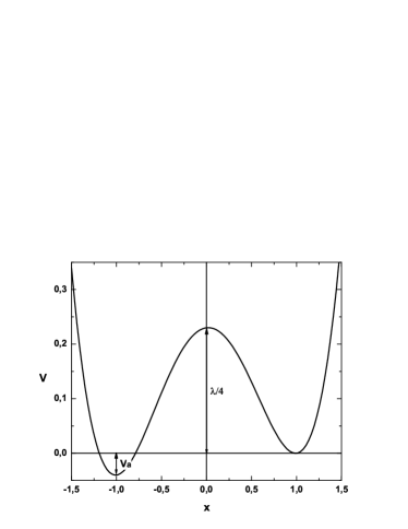
Figure 1: Various types of bistable potentials of the form given by Eq. (3) for $\lambda=1$. (a) symmetric potential $\Delta=0$; (b) asymmetric potential $\Delta=1$.

Note, such weakly asymmetric case, when right well is slightly higher than left one, corresponds smaller density of states in the right well than in the left one. Following Callan and Coleman [19] we call the phase corresponding to the minimum at position $x_{+}$ the false vacuum and the one corresponding to the minimum at position $x_{-}$ the true vacuum. Callan and Coleman presented an approach for analyzing the decay of an unstable vacuum in the framework of Euclidean quantum field theory.

For the system coupled to noisy reservoir the relevant Langevin equation of motion can be written as

$$\frac{\partial x}{\partial t}=-\frac{\partial V}{\partial x}+\varepsilon\left(t\right).$$ (4)

The first term corresponds to the dissipative term as well as the external applied force. The second term in Eq. (4) refers to an external additive noise. We assume that barier potential $\lambda$ fluctuates

$$V(x)=\frac{\lambda\left(t\right)}{4}\left(x^{2}-a^{2}\right)^{2}+\frac{\Delta}{a}\left(x-a\right),\lambda\left(t\right)=\lambda+\xi\left(t\right).$$ (5)

In general, we express the thermal fluctuation of the system as additive noise and the effect of the external environmental fluctuation on the system as multiplicative noise. A model with a fluctuating barrier and an additive noise was used in Ref. [20]. Linear fluctuations of the potential barrier were considered uncorrelated or correlated to the additive noise. The noises $\varepsilon\left(t\right)$ and $\xi\left(t\right)$ denote white Gaussian noises with zero mean and correlation function

$$\langle\varepsilon\left(t\right)\varepsilon\left(t+\tau\right)\rangle=2\epsilon^{2}\delta\left(\tau\right),$$ (6)

$$\langle\xi\left(t\right)\xi\left(t+\tau\right)\rangle=2\sigma^{2}\delta\left(\tau\right).$$ (7)

Hence the equation of motion can be obtained from Eq. (4) with using expression (5)

$$\frac{\partial x}{\partial t}=-\lambda x\left(x^{2}-a^{2}\right)-\frac{\Delta}{a}-x\left(x^{2}-a^{2}\right)\xi\left(t\right)+\varepsilon\left(t\right).$$ (8)

Below we assume Eq. (8) to be the Stratonovich stochastic differential equation with the supplementary condition

$$\langle\varepsilon\left(t\right)\xi\left(t+\tau\right)\rangle=\langle\xi\left(t\right)\varepsilon\left(t+\tau\right)\rangle=2\chi\epsilon\sigma\delta\left(\tau\right).$$ (9)

Value $\chi$ denotes the degree of correlation between additive $\varepsilon\left(t\right)$ and multiplicative $\xi\left(t\right)$ noises. The correlation between the multiplicative and additive noises realizes the hierarchical coupling of the system to the heat bath. Here $\epsilon$ and $\sigma$ are the strength of noises $\varepsilon\left(t\right)$ and $\xi\left(t\right)$, respectively.

3 Stationary probability distribution function

From equation (8) with conditions (6), (7) we can get the stochastic equivalent Langevin equation with one white-noise term [12]

$$\frac{\partial x}{\partial t}=\Phi\left(x\right)+\Gamma\left(x\right)\gamma\left(t\right),$$ (10)

where $\Phi\left(x\right)=-\lambda x\left(x^{2}-a^{2}\right)-\Delta/a$, and $\gamma\left(t\right)$ is a Gaussian white noise having zero mean magnitude and a delta-like correlation function

$$\langle\gamma\left(t\right)\gamma\left(t+\tau\right)\rangle=2\delta\left(\tau\right).$$ (11)

The expression for value $\Gamma\left(x\right)$ is determined by the following simple procedure: Let the correlation of $\Gamma\left(x\right)\gamma\left(t\right)$ in Eq. (10) be equal to the correlation of $-x\left(x^{2}-a^{2}\right)\xi\left(t\right)+\varepsilon\left(t\right)$ in Eq. (8). Following this approach, one can see that the required expression is

$$\Gamma\left(x\right)=\left[\sigma^{2}\varphi^{2}\left(x\right)+2\chi\epsilon\sigma\varphi\left(x\right)+\epsilon^{2}\right]^{1/2},$$ (12)

where

$$\varphi\left(x\right)=-x\left(x^{2}-a^{2}\right).$$ (13)

The equation (10) to be understood in the Stratonovich interpretation.

The Fokker-Plank equation corresponding to the stochastic differential equation (10) reads

$$\frac{\partial P\left(x,t\right)}{\partial t}=-\frac{\partial}{\partial x}\left\{\Phi\left(x\right)+\frac{1}{2}\frac{\partial}{\partial x}\left[\Gamma\left(x\right)\frac{\partial}{\partial x}\Gamma\left(x\right)\right]\right\}P\left(x,t\right).$$ (14)

This equation governs the time evolution of the system’s probability distribution $P\left(x,t\right)$ at time $t$. In the case of natural or instantly reflected boundary condition no probability current exists. The stationary probability distribution being

$$P_{st}\left(x\right)=N\cdot\exp\left\{\int_{0}^{x}du\frac{\Phi\left(u\right)-\Gamma\left(u\right)\Gamma^{\prime}\left(u\right)}{\Gamma^{2}\left(u\right)}\right\},$$ (15)

where $N$ denotes a normalization constant. The simplest way to analyze the stochastic dynamics of a system expressed by Eq.(10) is to take the Gibbs form of the stationary probability distribution function

$$P_{st}\left(x\right)\sim\exp\left\{-V_{eff}\left(x\right)\right\}.$$ (16)

The extrema of the effective potential $V_{eff}$ correspond to the stationary fixed points of the noise-sustained dynamics. For a bistable system, the probability distribution has two maxima which correspond to the stochastic steady states. Noted that the stationary probability distribution exhibits a symmetric bimodal structure for $\Delta=0$ and $\chi=0$.

4 Numerical simulation

We numerically simulated the double-well stochastic system described by Eq. (8). For that we employed the second-order stochastic Runge-Kutta type method (Heun’s algorithm) for integrating the dynamical equations of motion [21] with an integration time step $\Delta t=10^{-3}$. Gaussian white noise is generated using the Box-Muller algorithm. All calculated quantities are dimensionless.

Fig.2 displays the phase diagram of the model in the $\chi-\varepsilon$ and $\chi-\sigma$ parameter planes for fixed parameters $\sigma$ and $\varepsilon$ respectively.

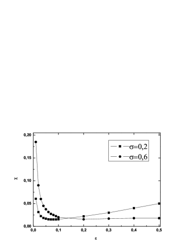
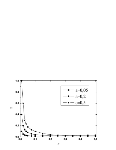
Figure 2: The phase diagram. (a) The plot of the degree of correlation $\chi$ between the multiplicative and additive noises vs the additive noise intensity $\varepsilon$ for fixed values of $\sigma$. (b) The plot of the degree of correlation $\chi$ between the multiplicative and additive noises vs the multiplicative noise intensity $\sigma$ for fixed values of $\varepsilon$.

The region with left maximum peak and right maximum peak are separated by a line of equal probability. On this line the potential $V_{eff}\left(x\right)$ is formal invariant under $x\rightarrow-x$ while the function $P_{st}\left(x\right)$ is a symmetric function of $x$. Thus noise suppressed of selection among broken-symmetry states. For $\sigma$ not too large the increase of the additive noise intensity causes the re-entrant ( symmetric-asymmetric-symmetric probability) transition.

In order to eliminate the influence of mutually correlated noises on the double-well system in Fig.3 we show the same curves in the $\chi-\lambda$ parameter planes. This representation clear indicate that for deep potential low degree of correlation between noises is quite enough for suppression of selection among broken-symmetry states. Moreover, the influence of additive noise $\varepsilon$ decreases with increase of $\lambda$.

Figure 3: Plot of $\chi$ vs $\lambda$ for fixed values of $\sigma$ and $\varepsilon$.

It must be emphasized that the lines in figures 2 to 3 correspond to stationary probability distribution function with symmetric maxima and separate two sectors corresponding a spontaneous breakdown of parity. As already mentioned, existence of cross-correlation between additive and multiplicative noises may lead to symmetrization of the stationary probability distribution. For $\chi=0$ and $\Delta\neq 0$ the shape of distribution is asymmetric.

5 Discussion

In this paper, we have analyzed the behavior of a double-well system under cross-correlated noises. In part, we have studied numerically for the lines corresponding to equal probability of maxima of this bistable system. We have shown that the cross-correlated noises suppressed of selection among broken-symmetry states. For $\sigma$ not too large this effect is re-entrant as a function of $\varepsilon$. Only the combined actions of the multiplicative noise and the additive noise causes such behavior. When the noises are uncorrelated, the stationary probability distribution exhibits an asymmetric bimodal structure for $\Delta\neq 0$ and a symmetric bimodal structure for $\Delta=0$.

References

- [1] J.R. Chaudhuri, S. Chattopadhyay and S.K. Banik, J. Chem. Phys. 128, 154513 (2008).
- [2] S.I. Denisov, A.N. Vitrenko, W. Horsthemke and P. Hänggi, Phys. Rev. E 73, 036120 (2006).
- [3] Y. Jin and W. Xu, Chaos, Solitons and Fractals 23, 275 (2005).
- [4] X. Luo and S. Zhu, Phys. Rev. E 67, 021104 (2003).
- [5] D. Mei, C. Xie, and L. Zhang, Phys. Rev. E 68, 051102 (2003).
- [6] B.C. Bag, Phys. Rev. E 66, 026122 (2002).
- [7] M. Gitterman, Phys. Rev. E 65, 031103 (2002).
- [8] L. Cao and D. J. Wu, Phys. Rev. E 62, 7478 (2000).
- [9] Y. Jia, S.-n. Yu, and J.-r. Li, Phys. Rev. E 62, 1869 (2000).
- [10] I.I. Fedchenia, J. Stat. Phys. 52, 1005 (1988).
- [11] A. Fulinski and T. Telejko, Phys. Lett. A 152, 11 (1991).
- [12] D.-j. Wu, L. Cao and S.-z. Ke, Phys. Rev. E 50, 2496 (1994).
- [13] A. J. R. Madureira, P. Hänggi and H.S. Wio, Phys. Lett. A 217, 248 (1996).
- [14] J.-h. Li and Z.-q. Huang, Phys. Rev. E 53, 3315 (1996).
- [15] Y. Jia and J.-r. Li, Phys. Rev. E 53, 5786 (1996).
- [16] S.Z. Ke, D.J.Wu and L. Cao, Eur. Phys. J. B 12, 119 (1999).
- [17] C.J. Tessone, H.S. Wio, and P. Hänggi, Phys. Rev. E 62, 4623 (2000).
- [18] Iu. Gudyma and B.Ivans’kii, Mod. Phys. Lett. B 20, 1233 (2006).
- [19] C.G. Callan and S. Coleman, Phys. Rev. D 16, 1762 (1977).
- [20] I.I. Fedchenia and N.A. Usova, Z. Phys. B 50, 263 (1983); 52, 69 (1983).
- [21] M.S. Miguel and R. Toral, in Instabilities and nonequilibrium structures VI, En.Tirapegui, J.Martinez and R.Tiemann, eds. (Kluwer Academic Publishers, Dordrecht, 2000), p. 35.