Threshold levels in Economics

Abstract

In this paper, we present theorems specifying the critical values for series associated with debts arranged in the order of their duration.

Key words: Crisis 2008, economic security, debts, duration, inflation.

1 Introduction

The mathematical theory used by economists up to now is probability theory and optimization theory. These theories cannot explain significant changes brought about by computerization just as, at the beginning of the 20th century, the classical physics could not interpret new experiments.

Nowadays the mathematical background of economics is the so-called complexity theory (A. N. Kolmogorov, 1956) and the closely-related theory of mathematical prediction (R.Solomonoff, 1964) as well as some other arithmetic (addition rules) introduced by the author [1].

The threshold values guaranteeing economic security, which are cited by the economists, are rather nebulous (see for example [2]).

These values correspond to the violation of economic security, while it is of interest to find the threshold values beforehand so that correction measures can be taken.

Let me give a simple example of a critical number. Recall the “trick” of Korovjev, aka Fagot, in the novel “Master and Margarita” by Mikhail Bulgakov. Banknotes of 10-ruble denomination were scattered among the spectators at a variety show. We assume that all the variants of permutation of $n$ banknotes among $k$ spectators are equiprobable (the chaos assumption). In that case, if the number of spectators is greater than $\sqrt{n}lnn$, then there is a large probability that $k-\sqrt{n}lnn$ spectators will not get anything at all.

But if the spectators are combined into groups so that the number of groups is $\sqrt{n}$, then there is a large probability that all the groups will get some banknotes, which will be than divided in a friendly manner among all the members according to the rules of ordinary arithmetic. This represents the amount of intervention of ordinary arithmetic (state management) into the arithmetic of a chaotic market, which is determined by the excess of indicators over the corresponding critical number.

In real economics, corporate bodies (firms), not natural persons, are analogs of the spectators. Laws of ordinary arithmetic and planning act within each firm where there is no economic competition. But there is economic competition among firms. State regulatory intervention is necessary in cases where the critical number is exceeded and some firms go bankrupt.

In the case of the bankruptcy of a firm, its employees become unemployed. And, in that case, it is up to the state to take care of them, otherwise, there may be trouble for the employed citizens. Therefore, the state must intervene in free economic relations and plan the corresponding actions where necessary. The amount of such intervention depends on the excess of the predicted value over the critical number.

As I have already pointed out on numerous occasions, another way to fight the “inexorable law of numbers” is to introduce a multi-currency system, which increases the barter component .

Let me give an example.

Suppose we want to deposit two kopecks in two different banks (see [3]; then we can say that there are three possibilities: (1) put both kopecks into one of the banks; (2) put both kopecks into the other bank; (3) one kopeck in one bank, the other, in the other one. Here it is of no consequence which of the two coins we deposit in the first bank and what is its year of issue. Now imagine a situation in which we are depositing one kopeck and one pence instead of two kopecks. In that case, we have four options rather than three, because it is significant which coin we placed in what bank, and so the variant in which the coins are placed in different banks yields two different options: (a) one kopeck to bank 1 and one pence to bank 2; (b) one kopeck to bank 2 and one pence to bank 1.

The first case corresponds to the Bose–Einstein statistics that leads, as is well known, to the Bose–Einstein condensate. In financial mathematics, this phenomenon [4] yields threshold values. In the second case, the number of variants corresponds to the Boltzmann statistics, which, however, does not encompass such a phenomenon.

Let me give a second example. The members of a family wish to change their flat into two flats. Nowadays, in Russia, the flat in question is sold and then two flats are bought with the help of real-estate agencies. This procedure takes at least two months. In Soviet times, there were long exchange chains, which can now be optimized using computers and data bases. If the price of flats rapidly changes during the flat-exchange process, then, due to the uniform variation of prices, the parties do not lose anything if all the flats are exchanged at the same time. Since such an exchange chain corresponds to the Boltzmann statistics, there is no Bose condensate.

There is yet another method, which was described in Bulgakov’s novel: the 10-ruble banknotes turned into sweet wrappers. But, in that case, there is no more trust in 10-ruble banknotes, which leads to a downturn in the economy, as is happening now in our country where the banks are afraid of giving out ruble credits.

If the government does not intervene, then such processes may occur spontaneously, leading to undesirable losses. There is no way to avoid mathematical laws. As Admiral Kolchak put it, there is “this inexorable law of numbers” by which he apparently meant superiority in numbers.

The separation of the money supply from the debt total is an approximation just as the quantum statistical physics of bosons is an approximation of scalar quantum field theory in its Hamiltonian version[5, 6, 7]. In the latter theory, particles and holes can be created and annihilated in the same way as money annihilates debts.

There is also a rapid turnover in debts; they are annihilated and created anew. However, in the mean, both debts and assets are quite obvious even more so than money and money turnover.

If we use an electronic bank card for payments, then this increases the rate of turnover in the same way as e-mail increases the postal delivery rate. However, we must find the weak limit with respect to these rapid variations so as to obtain threshold values to be discussed in what follows.

The concept of the mean rate of turnover defined in textbooks in economics as the ratio of GDP to the amount of the available money was meaningful only in the case of gold coins. But, nowadays, it is the same weak limit, which is practically used when in estimating bank assets.

In the same way, in the thermodynamic limit of the total system, the number of particles $N^{+}$ and holes $N^{-}$ is preserved (the model of ions–electrons in a plasma; see [8]). Hence the sum

$$N^{+}+N^{-}=N_{\text{total}}$$ (1)

is also preserved.

But if we consider a subsystem in which the number $N^{-}$ has increased due to external action, then, in the first equilibrium approximation, it turns out that $N_{\text{total}}$ is preserved, and hence $N^{+}$ is decreased. At the same time, the total energy after deduction of the infinite energy of vacuum is preserved. Approximately,

$$\varepsilon\sum_{-k}^{\infty}iN_{i}=\cal{E},$$ (2)

where $\cal{E}$ is the total energy, $\varepsilon$ is the energy of one particle, and

$$\sum_{i=-k}^{\infty}N_{i}=N.$$ (3)

Making the replacement $i+k=j$, we obtain

$$\varepsilon\sum_{j=0}^{\infty}(j-k)N_{j-k}=\cal{E}.$$ (4)

Taking (3) into account, we can write

$$\varepsilon\sum_{i=0}^{\infty}iN_{i}={\cal E}+\frac{k(k+1)}{2}\,N\varepsilon.$$ (5)

Here the term $k(k+1)/2$ tends to infinity as $k\to\infty$. This is the analog of the energy of vacuum, which must be deducted. A rigorous proof of passages to the limit with deduction of infinities is difficult. An attempt to justify these passages mathematically (such as the passage to nonrelativistic quantum field theory) was made in [5], [6], and [7].

How to interpret the law of conservation of the sum $N^{+}+N^{-}$ (the sum of assets and liabilities) in economics? Although a significant role in economics is played by the psychological factor, this law, nevertheless, corresponds to mathematical laws in the mean (after averaging over subjects and time).

Let us assume that a young family borrows some money for education, mortgage, and a car. This stimulates the family to earn more money. If one-half of the increased income is used to repay the loan, and the other half goes toward increasing the assets, then we have $N^{+}+N^{-}=\text{const}$.

Debts and assets treated separately are, in fact, the result of averaging over rapid transitions “credits$\leftrightarrow$incomes.”

In practice, both debts (liabilities) and money (assets) are calculated, although, as pointed out above, they are averaged over rapidly varying turnovers “money$\leftrightarrow$debts.”

Therefore, pre-crisis American banks can be associated with, for example, the time series of their assets and they can be classified according to the size of their assets. The journal “Forbes” classifies the richest people by the mean size of their fortune. From a mathematical point of view, we are not interested in the names of persons or banks, but in their numbers ordered in the same way as in “Forbes,” beginning with the greatest fortune, and also their variation over sufficiently large time intervals. Only from these time series, can we determine economic threshold values by using the theorems given below in this paper.

Let us begin by considering debts. In addition to other features of a debt, such as the percentage, each debt $s$ is characterized by its period of repayment (pay-out period) $l$. The ratio of the debt size to its pay-out period is the quantity of immediate interest to the borrower, because it determines the amount of extra effort per day needed to repay the debt in time. If there are debts $s_{i}$, $i=1,2,\dots,k$, with pay-out periods $l_{i}$, then the sum of the ratios of debts to their pay-out periods represents the amount of extra money to be earned each day. The ratio of $\sum_{i=1}^{k}s_{i}/l_{i}$ to the amount of all the debts $\sum_{i=1}^{k}s_{i}$ is the mean period of repayment of all debts.

Here we present a criterion and a certain critical constant (threshold level). If the mean period of repayment of debts is greater than this level, then the borrower is bankrupt. This quantity is just as precise as the number of spectators at Koroviev’s performance; the important thing is that it depends on quantities specified by the series $\{s_{i}\}$ and $\{s_{i}/l_{i}\}$. This looks like a mathematical mystery. However, this phenomenon is related to a remarkable physical fact, namely, the existence of the Bose–Einstein condensate for a Bose gas. In our case, this means that if this number is greater than the critical number, then the debts turn out to be long-term ones, which usually are mortgages.

People did not believe in this physical phenomenon for a long time, but, finally, got used to it. And there exist many experiments that confirm this phenomenon. In deterministic physics, it has no easy explanation. But there is an explanation in economics. There are few experiments involving a crisis: it seems that there is just one such world-wide experiment. In this sense, economics can enrich physics, just as it helped the author to explain the so-called $\lambda$-point in the Bose condensate of Helium-4 and the Thiess–Landau model (see below).

The war in Iraq required substantial loans, mostly internal ones (such as from insurance companies) and a subsystem (financial bodies and the defence industry) having received $N^{-}$ credits (debts, holes) decreased the number of particles (the total energy being constant) according to the law (1); this means that the turnover of particles (the Bose-gas temperature) increased or, as the economists put it, the subsystem has heated up and there began an abrupt upturn in the economy of the subsystem. Naturally, this resulted in an increase of mortgage (floating) interests, while most of the people living in mortgaged houses was not involved in the system where incomes were growing. Hence the mortgage crisis occurred and this was followed by the crisis of insurance companies dealing with mortgages (and also long-term credits), etc. This is a rather deterministic explanation of Bose condensate. It is up to physicists and, especially, specialists in mathematical physics to try to carry over this explanation to scalar Hamiltonian field theory and use it for the deduction of the Bose-condensate phenomenon.

Let us now turn to the opposite phenomenon, inflation (it is opposite in the sense that, as shown above, the debt crisis leads to deflation).

Here the situation is more complex, but it easily explains inflation at the time when the currency was in the form of gold coins. One could also calculate the GDP at that time, but, in contrast to the present time, one could calculate the number of gold coins in circulation more precisely (although bills of credit were also used, but they could hardly be used to buy goods in a shop; they could be bought up in order to bring about a bankruptcy). At present, banknotes are seldom used in shops abroad, mostly bank cards and cheques, which, in fact, are bills of credit.

Therefore, in textbooks on economics, there is a tradition of long standing to state the main law of economics as follows: the mean rate of turnover of money (gold coins) is equal to the ratio of the GDP to the total number of gold coins.

The GDP of a country is composed of similar quantities associated with its constituent parts (regions) and these quantities, in turn, involve quantities corresponding to finer structures. In such series, one can precisely calculate the threshold turnover rate possessing the following property: if the mean turnover rate is less than this threshold value, then inflation occurs, as a result of which smaller coins (copecks in Russia) are no longer used, while gold coins disappear into money boxes or chests.

Remark 1.

All the critical constants given above are highly sensitive to a phenomenon called “protectionism.”

Suppose that, in our example, Koroviev took pity on those spectators that did not get any banknotes and he gave them one banknote in “aid.” Thus, he changed the situation by equating such people to those who got one banknote by the “market” law. This is the same as if the unemployment benefit were raised to the level of the wages of some categories of workers. Then these workers would find themselves to be on the same “zero” level of unemployed persons.

If the debts of the debtors are restructured to a longer period, then those who took credits (such as mortgage) for such long periods are threatened.

Then the kind Koroviev should have added some money to those spectators who had grabbed just one banknote. Thus, if credit owners suffer as a result of “protectionism,” they should be the ones to get help in the first place.

Since the law of conservation of energy in the physics of particles–holes–photons that are created and annihilated at a great rate is valid in the mean, it follows that the number of particles and holes is preserved in the mean, too. Despite a tremendous rate of debts–money transitions, in modern computer economics, assets and liabilities are preserved in the mean in the weak limit, and we can consider the time series of these quantities.

2 Koroviev’s trick and partition theory in number theory

Let us return to Koroviev’s trick.

Assume that there were $n$ banknotes and $k$ persons in the audience, where

$$k>\frac{1}{\pi}\sqrt{\frac{3}{2}}\sqrt{n}\ln n$$.

We certainly assume that all versions of distributing $n$ banknotes among $k$ persons are equiprobable. Let us state a theorem of number theory.

Let $n$ be a positive integer. By a partition of $n$ we mean a way to represent a natural number $n$ as a sum of natural numbers. Let $p(n)$ be the total number of partitions of $n$, where the order of the summands is not taken into account, i.e., partitions that differ only in the order of summands are assumed to be the same. The number $p_{k}(n)$ of partitions of a positive integer $n$ into $k$ positive integer summands is one of the fundamental objects of investigation in number theory.

In a given partition, denote the number of summands (in the sum) equal to 1 by $N_{1}$, the number of summands equal to 2 by $N_{2}$, etc., and the number of summands equal to $i$ by $N_{i}$. Then $\sum N_{i}=k$ is the number of summands, and the sum $\sum iN_{i}$ is obviously equal to the partitioned positive integer. Thus, we have

$$\sum_{i=1}^{\infty}iN_{i}=n,\qquad\sum_{i=1}^{\infty}N_{i}=k,$$ (6)

where the $N_{i}$ are natural numbers not exceeding $k$.

These formulas can readily be verified for the above example. Here all the families $\{N_{i}\}$ are equiprobable.

The distribution for the parastatistics $N_{i}\leq k$ and $\sum N_{i}=k$ is determined from the relations

$$\sum_{i=1}^{n}\frac{1}{e^{b(i+\kappa)}-1}-\frac{k}{e^{bk(i+\kappa)}-1}=k,\qquad\sum_{i=1}^{n}\bigg{(}\frac{i}{e^{b(i+\kappa)}-1}-\frac{ik}{e^{bk(i+\kappa)}-1}\bigg{)}=n,$$ (7)

where $b>0$ and $\kappa>0$ are constants defined from relations (7), $n/k$ is sufficiently large, and the numbers $n$ and $k$ are also large, and we can pass (by using the Euler–Maclaurin summation formula) to the integrals (for the estimates for this passage, see [9]),

$$\int_{0}^{\infty}\bigg{(}\frac{1}{e^{b(x+\kappa)}-1}-\frac{k}{e^{bk(x+\kappa)}-1}\bigg{)}\,dx \cong k,$$ (8)

$$\int_{0}^{\infty}\bigg{(}\frac{x}{e^{b(x+\kappa)}-1}-\frac{kx}{e^{bk(x+\kappa)}-1}\bigg{)}\,dx \simeq n.$$ (9)

It can be proved that $\kappa=0$ gives the number $k_{0}$ with satisfactory accuracy. Hence,

$$k_{0}=\int_{0}^{\infty}\bigg{(}\frac{1}{e^{bx}-1}-\frac{k_{0}}{e^{bk_{0}x}-1}\bigg{)}\,dx.$$

Consider the value of the integral (with the same integrand) taken from $\varepsilon$ to $\infty$ and then pass to the limit as $\varepsilon\to 0$. After making the change $bx=\xi$ in the first term and $bk_{0}x=\xi$ in the second term, we obtain

$$k_{0} =\frac{1}{b}\int_{\varepsilon b}^{\infty}\frac{\,d\xi}{e^{\xi}-1}-\int^{\infty}_{\varepsilon bk_{0}}\frac{\,d\xi}{e^{\xi}-1}=\frac{1}{b}\int^{\varepsilon bk_{0}}_{\varepsilon b}\frac{\,d\xi}{e^{\xi}-1}$$ (10)

$$\sim\frac{1}{b}\int^{\varepsilon bk_{0}}_{\varepsilon b}\frac{\,d\xi}{\xi}=\frac{1}{b}\{\ln(\varepsilon bk_{0})-\ln(\varepsilon b)\}=\frac{1}{b}\ln k_{0}.$$ (11)

On the other hand, making the change $bx=\xi$ in (9), we obtain

$$\frac{1}{b^{2}}\int^{\infty}_{0}\frac{\xi\,d\xi}{e^{\xi}-1}\cong n.$$

This gives

$$b=\bigg{(}{\sqrt{n}}\bigg{/}{\sqrt{\int_{0}^{\infty}\frac{\xi\,d\xi}{e^{\xi}-1}}}\,\bigg{)}^{-1},\qquad k_{0}=\frac{1}{2}\frac{\sqrt{n}}{\sqrt{\pi^{2}/6}}\ln n(1+o(1)).$$ (12)

Now let us find the next term of the asymptotics by setting

$$k_{0}=c^{-1}n^{1/2}\ln c^{-1}n^{1/2}+\alpha n^{1/2}+o(n^{1/2}),\qquad\text{where}\quad c=\frac{2\pi}{\sqrt{6}}\,.$$

Furthermore, using the formula

$$k_{0}=c^{-1}n^{1/2}\ln k_{0}$$

and expanding $\ln k_{0}$ in

$$\frac{\alpha}{c^{-1}\ln c^{-1}n^{1/2}}\,,$$

we obtain

$$\alpha=-2\ln\frac{c}{2}$$.

Thus, we have obtained the Erdős formula [10].

Let us show that, if $k>k_{0}$, then $\kappa<\nobreak 0$.

Lemma 1.

Let $n>k\gg k_{0}$. Suppose that $\kappa=-\mu$ and $\mu>0$. In this case, equations (8) and (9) have solutions with $\mu>k^{-1/2-\delta}$, where $\delta>\nobreak 0$ is as small as desired.

Proof.

Indeed, consider relations (8) and (9). Making the change $\xi-\mu=\eta$, and then $b\eta=\varphi$, we obtain

$$n =\frac{1}{b^{2}}\int_{0}^{\mu}\frac{k\xi\,d\xi}{1-e^{-k\xi}}-\frac{1}{b^{2}}\int_{0}^{\mu}\frac{\xi\,d\xi}{1-e^{-\xi}}+\frac{1}{b^{2}}\int_{0}^{\infty}\bigg{(}\frac{\xi}{e^{\xi}-1}-\frac{k\xi}{e^{k\xi}-1}\bigg{)}\,d\xi,$$ (13)

$$k =\frac{1}{b}\int_{\varepsilon}^{\mu}\bigg{(}\frac{k}{1-e^{-k\xi}}-\frac{1}{1-e^{-\xi}}\bigg{)}\,d\xi+\frac{1}{b}\int_{\varepsilon}^{\infty}\bigg{(}\frac{1}{e^{\xi}-1}-\frac{k}{e^{\xi k}-1}\bigg{)}\,d\xi.$$ (14)

After making the change $k\xi=x$ in the corresponding integrals, we see that

$$n =\frac{1}{b^{2}}\frac{1}{k}\int_{0}^{\mu k}\frac{x\,dx}{1-e^{-x}}+o\bigg{(}\frac{1}{b^{2}}\bigg{)},$$ (15)

$$k =\frac{1}{b}\int_{0}^{\mu k}\frac{\,dx}{1-e^{-x}}+o\bigg{(}\frac{\ln k}{b}\bigg{)}$$ (16)

as $k\to\infty$. Therefore, $\mu k\ll\sqrt{k}$; for instance, $\mu k\geq\sqrt{k^{1-\delta}}$ for any $1>\delta>0$.

This relation can be satisfied provided that $\mu>(\sqrt{k^{1+\delta}})^{-1}$. This proves the lemma. ∎

The logarithm of the number of variants is the Hartley entropy, and the entropy for a parastatistic is known.

$$S(k_{0})\sim bn+\int_{0}^{\infty}\ln\frac{1-e^{-(k+1)bx}}{1-e^{-bx}}\,dx.$$ (17)

But if $\kappa<0$, the entropy is of the form

$$S(k)=bn-\kappa k+\sum_{j=1}^{\infty}\ln\frac{1-e^{-(k+1)b(j-\kappa)}}{1-e^{-b(j-\kappa)}}\sim bn-\kappa k+\int_{0}^{\infty}\ln\frac{1-e^{-(k+1)b(x-\kappa)}}{1-e^{-b(x-\kappa)}}\,dx.$$ (18)

Lemma 2.

The ratio

$$\frac{p_{k}(n)}{p_{k_{0}}(n)}=e^{S(k)-S(k_{0})}\geq e^{-(\mu k)^{1-\delta}},$$ (19)

where $\delta>0$.

Proof.

We can write

$$S(k) =bn-\mu k+\int_{-\mu}^{0}\ln\frac{1-e^{-(k+1)b\xi}}{1-e^{-b\xi}}\,d\xi+\int_{0}^{\infty}\ln\frac{1-e^{-(k+1)bx}}{1-e^{-bx}}\,dx$$

$$=S(k_{0})-\mu k+\int_{0}^{\mu}\ln\frac{e^{(k+1)b\xi}-1}{e^{b\xi}-1}\,d\xi.$$ (20)

The estimate

$$\int_{0}^{\mu}\ln\frac{e^{(k+1)b\xi}-1}{e^{b\xi}-1}\,d\xi$$

yields the assertion of Lemma 2 after the calculation of the maximum of the expression under the sign of logarithm. ∎

A rigorous proof of the weak convergence to the Bose–Einstein distribution of sequences corresponding to an ideal Bose gas of dimension greater than two is given in a remarkable work of A. Vershik [11]. For the dimension $d\leq 2$, this proof is valid for the parastatistic discussed above. The following theorem holds.

Theorem 2.1.

1) Suppose that $p_{k}(n)$ is the number of partitions of an integer $n$ into $k\leq k_{0}$ summands and $N_{i}$ is the number of occurrences of the integer $i\leq k$ in these partitions. Then the difference

$$b\sum_{i=1}^{k}N_{i}\varphi(bi)-\int_{0}^{\infty}\varphi(x)\left\{\frac{1}{e^{x+\kappa}-1}-\frac{k}{e^{k(x+\kappa)}-1}\right\}\,dx,$$ (21)

where the function $\varphi(x)$ is any bounded piecewise smooth (with finitely many discontinuities) function continuous at the points $bi$, tends in probability to zero as $k\to\infty$.

2) Let $k>k_{0}+o(k_{0})$, and suppose that $k_{0}$ spectators got at least one bank note each; hence the distribution (21) is valid for them. Let $N_{0}$ be the number of spectators without bank notes. In that case, obviously,

$$P\left(|N_{0}-(k-k_{0})|>\delta_{1}k_{0}\right)\leq e^{-(k-k_{0})^{1/2-\delta}},$$ (22)

where $\delta>0$ and $\delta_{1}>0$ are arbitrarily small and do not depend on $n$. Here $P$ is the ratio of the number of variants satisfying the condition in parentheses in (22) to $p_{k_{0}}(n)$.

Further, the occurrence of the numbers $i\leq A/b$, where $A$ is an arbitrarily large number independent of $b$, satisfies the relation

$$b\sum_{i=1}^{[A/b]}N_{i}\varphi(bi)-\int_{0}^{\infty}\varphi(x)\left\{\frac{1}{e^{x}-1}-\frac{k_{0}}{e^{k_{0}x}-1}\right\}\,dx\xrightarrow{\mathsf{P}}0\qquad\text{as}\quad n\to\infty.$$

Proof.

The formula for the parastatistic

$$R(x)=\int_{0}^{x}\bigg{(}\frac{1}{e^{b(x+\kappa)}-1}-\frac{k}{e^{bk(x+\kappa)}-1}\bigg{)}\,dx,$$

given in physics textbooks obviously follows from the rigorous relation for the parastatistic and Stirling’s decomposition formula. Sharper estimates [12] are not needed for the proof.

Our further proof is quite similar to that of Vershik’s theorem [11].

The use of the Euler–Maclaurin theorem and estimates for the passage from sums to integrals yields Theorem 1.

For $k\leq\sqrt{n}$, using the Banach–Steinhaus theorem, we can obtain weak convergence in formula (21).

The proof of inequality (22) follows from Lemmas 1 and 2, because, by performing the change $N_{0}=k-(k_{0}+o(k_{0}))$, we do not change the number of partitions ${p_{k_{0}}(n)}$. ∎

Remark 2.

In physics, the parameter $b$ is called inverse temperature and the parameter $\kappa$ is the chemical potential taken with a negative sign; the dimension $d$ of the space in which a quantum ideal gas is considered is two in our case.

With regard to the value of the dimension, we shall follow the physics literature in contrast to [3], where dimension was defined as the quantity half as large as the physical dimension. The quantity $d$ can be associated with the so-called Pareto distribution and its rate of decrease. It is related to spectral density.

In the physics literature, it is universally stated (in contrast to [13]) that there is no Bose condensate in the two-dimensional case (for $d=2$). The same statement is contained in [11]. Indeed, formally, it is not a Bose condensate, but the condensate of a parastatistic.

Let us consider a financial example in which the dimension $d=2$ occurs.

Example 1.

Japanese candles on the stock exchange. On the stock exchange, the data on prices in a given time scale (such as hour intervals) is given as four prices: opening price, highest price, lowest price, and closing price. This allows reduction in the amount of stored data as well in the time of their processing.

These four prices are usually represented as “Japanese candles.” The extreme points of the upper and lower segments denote, respectively, the highest and the lowest price for a given day, while the upper and the lower base of the rectangle (body of the candle) denote, respectively, the opening and closing prices if the rectangle is white and the closing and opening prices if the rectangle is black (see Fig. 6.3/1 in [3])

Thus, the Japanese candle is the symbol indicating the variation of the price of a particular financial tool (share) on the stock exchange. We shall number them in decreasing order of frequency.

Not only Japanese candles on the stock market, but also the whole world financial system relies on the positive values of $\kappa$ ($\kappa>0$), provided that $\kappa\to 0$ as $b\to 0$. Then it demonstrates a sufficiently rapid growth. However, no wars must break out; for $\kappa<\nobreak 0$, they may lead to the global financial catastrophe.

Lately, there is a growing tendency to group shares into equivalent sets (similar to grouping words into descriptors). For an investor, shares of one group may replace one another just as pronouns and rare synonyms may replace repeating words and thus change the statistics describing the occurrence of words. Investors try to avoid repetition to a greater degree than do writers, who try to prevent the repetition of the same words: the greater the range of goods bought, the less the risk to incur losses. The rank on the graph 6.3/2 from [3]) is the number of a candle (numbered in ascending order with respect to candle size); in this case, the fractal dimension $\alpha$ is $1$.

Figuratively speaking, if the spectators in our example with the conjuring trick are divided into groups so that the number of groups is greater than the critical number, but exceeds it by only a small amount, then the spectators in each group will be nervous about the amount of bank notes they will be getting, and hence will be active. But if it turns out that the number of groups is much less than the critical number, than the spectators will be sure that they will get a lot of bank notes with large probability, and hence will be passive, or as P. Milyukov put it, they will “bask in the state of blissful idiotism” or, which is still worse, become obscurantists.

3 The dimensions $d=1$ and $0<d<2$

Just as above, let us consider the dimension $d=1$. If, in physics, the dimension $d=2$ corresponds to a plane, then the dimension $d=1$ corresponds to a line.

First, consider the one-dimensional case of a Bose condensate, which is important in physical problems, in the notation used in statistical physics: $\cal E$ is the energy, $k=N$ is the number of particles, $\varepsilon i$ are the energy levels, and $n={\cal E}/{\varepsilon}$.

Let the dimension be $d=1$.

Define the constants $b$ and $\kappa$ from the following relations:

$$\varepsilon\int_{0}^{\infty}\xi\left(\frac{1}{e^{b(\xi+\kappa)}-1}-\frac{N}{e^{bN(\xi+\kappa)}-1}\right)d\sqrt{\xi} =\cal E,$$ (23)

$$\int_{0}^{\infty}\left(\frac{1}{e^{b(\xi+\kappa)}-1}-\frac{N}{e^{bN(\xi+\kappa)}-1}\right)d\sqrt{\xi} =N.$$ (24)

First, let us determine $b$ from the relation

$$n=\frac{1}{2}\int_{0}^{\infty}\frac{\sqrt{\xi}\,d\xi}{e^{b\xi}-1}=\frac{1}{b^{3/2}}\int_{0}^{\infty}\frac{\sqrt{\xi}\,d\xi}{e^{\xi}-1}\,.$$ (25)

Hence

$$b=\frac{1}{(2n)^{2/3}\left(\int^{\infty}_{0}\frac{\sqrt{\xi}\,d\xi}{e^{\xi}-1}\right)^{2/3}}\,.$$ (26)

We use the following identity:

$$\int^{\infty}_{0}\left(\frac{1}{x^{2}}-\frac{1}{x^{2}(1+\alpha x^{2})}\right)\,dx=\sqrt{\alpha}\int_{0}^{\infty}\frac{\,d\xi}{1+\xi^{2}}\,.$$ (27)

Let us find $N_{cr}$ from the relation

$$N_{cr}=\frac{1}{2}\int\left(\frac{1}{\sqrt{\xi}(e^{b\xi}-1)}-\frac{N_{cr}}{\sqrt{\xi}e^{bN_{cr}\xi}-1}\right)\,d\xi=\frac{1}{\sqrt{b}}\int_{0}^{\infty}\left(\frac{1}{e^{\xi^{2}}-1}-\frac{N_{cr}}{e^{\xi^{2}N_{cr}}-1}\right)\,d\xi.$$ (28)

Subtracting ${1}/{\xi^{2}}$ from both terms of the difference, we obtain $k_{0}=N_{cr}=k_{0}$, which determines the transition to the Bose condensate,

$$k_{0} =\frac{1}{\sqrt{b}}\int\left(\frac{1}{e^{\xi^{2}}-1}-\frac{1}{\xi^{2}}\right)+\frac{1}{\sqrt{b}}\int\left(\frac{1}{\xi^{2}}-\frac{1}{\xi^{2}(1+\frac{k_{0}}{2}\xi^{2})}\right)\,d\xi$$

$$\qquad-\frac{1}{\sqrt{b}}\int\left(\frac{k_{0}}{e^{k_{0}\xi^{2}}-1}-\frac{k_{0}}{k_{0}\xi^{2}(1+\frac{k_{0}}{2}\xi^{2})}\right)\,d\xi.$$ (29)

In view of the relations

$$\frac{1}{\sqrt{b}}\int\left(\frac{k_{0}}{e^{k_{0}\xi^{2}}-1}-\frac{k_{0}}{k_{0}\xi^{2}(1+\frac{k_{0}}{2}\xi^{2})}\right)\,d\xi=\frac{\sqrt{k_{0}}}{\sqrt{b}}\int_{0}^{\infty}\left(\frac{1}{e^{\eta^{2}}-1}-\frac{1}{\eta^{2}(1+\frac{\eta^{2}}{2})}\right)d\eta$$ (30)

and

$$\frac{1}{\eta^{2}(1+\frac{\eta^{2}}{2})}=\frac{1}{\eta^{2}}-\frac{1}{2}\frac{1}{(1+\frac{\eta^{2}}{2})}$$ (31)

solving the quadratic equation for $x=\sqrt{k_{0}}$, we obtain $k_{0}\approx 4c^{2}n^{2/3}$, where

$$c=\int_{0}^{\infty}\left(\frac{1}{e^{\xi^{2}}-1}-\frac{1}{\xi^{2}}\right)\,d\xi\left(\frac{1}{2}\int_{0}^{\infty}\frac{\sqrt{\xi}\,d\xi}{e^{\xi}-1}\right)^{2/3},$$

Lemma 3.

Let $n>k\gg k_{0}$. Suppose that $\kappa=-\mu$ and $\mu>0$. In this case, Eqs. (23) and (24) have the solutions $k^{-1/3}\gg\mu>k^{-1/3-\delta}$, where $\delta>\nobreak 0$ is arbitrarily small.

Consider relations (23) and (24). Making the change of variables $\xi-\mu=\eta$ and then $b\eta=\varphi$, we obtain

$$n =\frac{1}{b^{3/2}}\int_{0}^{\mu}\frac{k\xi d\sqrt{\xi}}{1-e^{-k\xi}}-\frac{1}{b^{3/2}}\int_{0}^{\mu}\frac{\xi d\sqrt{\xi}}{1-e^{-\xi}}+\frac{1}{b^{3/2}}\int_{0}^{\infty}\left(\frac{\xi}{e^{\xi}-1}-\frac{k\xi}{e^{k\xi}-1}\right)d\sqrt{\xi},$$ (32)

$$k =\frac{1}{\sqrt{b}}\int_{\varepsilon}^{\mu}\left(\frac{k}{1-e^{-k\xi}}-\frac{1}{1-e^{-\xi}}\right)d\sqrt{\xi}+\frac{1}{\sqrt{b}}\int_{\varepsilon}^{\infty}\left(\frac{1}{e^{\xi}-1}-\frac{k}{e^{\xi k}-1}\right)d\sqrt{\xi}.$$ (33)

After making the change $k\xi=x$ in the corresponding integrals, we see that, as $k\to\infty$,

$$n =\frac{1}{b^{3/2}}\frac{1}{\sqrt{k}}\int_{0}^{\mu k}\frac{xd\sqrt{x}}{1-e^{-x}}+o\left(\frac{1}{b^{3/2}}\right),$$ (34)

$$k =\frac{1}{\sqrt{b}}\int_{\mu}^{\mu k}\frac{d\sqrt{x}}{1-e^{-x}}+o\left(\frac{\ln k}{\sqrt{b}}\right).$$ (35)

Hence $(\mu k)^{3/2}\ll\sqrt{k}$; in particular, $k\gg(\mu k)^{3}>k^{1-\delta}$ for any $1>\delta>0$.

The estimate of the entropy is similar to that in Lemma 2.

Theorem 3.1.

1) Suppose that $N_{i}$ is the number of particles on the level $\varepsilon i$, $N\leq k_{0}$, and all the variants $\{N_{i}\}$ satisfying the condition

$$\sum_{i=1}^{\infty}{N_{i}}=N$$,

are equiprobable under the condition

$$\varepsilon\sum_{i=0}^{\infty}|i|^{2}N_{i}=\cal{E}$$.

Then the difference

$$b^{1/2}\sum_{i=1}^{\infty}N_{i}\varphi(bi)-\frac{1}{2}\int_{0}^{\infty}\varphi(x)\frac{1}{|x|^{1/2}}\left\{\frac{1}{e^{x+\kappa}-1}-\frac{N}{e^{N(x+\kappa)}-1}\right\}\,dx,$$ (36)

where the function $\varphi(x)$ is any bounded piecewise smooth function continuous at the points $bi$, tends in probability to zero as $N\to\infty$.

2) Now let $N>k_{0}+o(k_{0})$.

The ratio of the number of variants in which the number $N_{0}$ of particles in the condensate occurs more rarely than the number

$$N-4c^{2}n^{2/3}-o(n^{2/3}),$$ (37)

where

$$c=\int_{0}^{\infty}\left(\frac{1}{e^{\xi^{2}}-1}-\frac{1}{\xi^{2}}\right)\,d\xi\left(\frac{1}{2}\int_{0}^{\infty}\frac{\sqrt{\xi}\,d\xi}{e^{\xi}-1}\right)^{2/3},$$

to the total number of variants tends to zero faster than

$$e^{-(N-4c^{2}n^{2/3})^{1/3-\delta}},$$

where $\delta$, $1/2>\delta>0$, is any arbitrarily small number independent of $N_{0}$.

Now consider the case of the dimension $0<d<2$.

What does it mean from from the viewpoint of Koroviev’s conjuring trick? Suppose that tickets were sold for different prices. The most expensive ticket provides its owner with the largest area $S_{\max}$ in the auditorium and, therefore, the largest area for collecting the bank notes. The prices of other tickets decrease monotonically with the size of the area alotted to spectators. If all the areas are the same and equal to $S_{\max}$, as in Koroviev’s trick, then we have the situation considered in Theorem 1, which corresponds to dimension $d=2$. But if the areas decrease in size, then the dimension is $d<2$. Let us find the threshold numbers in this situation.

Let us find constants $b$ and $\kappa$ from the following relations:

$$\int_{0}^{\infty}\xi\left\{\frac{1}{e^{b(\xi+\kappa)}-1}-\frac{k}{e^{bk(\xi+\kappa-1)}}\right\}d\xi^{\alpha} =n,$$ (38)

$$\int_{0}^{\infty}\left\{\frac{1}{e^{b(\xi+\kappa)}-1}-\frac{k}{e^{bk(\xi+\kappa-1)}}\right\}d\xi^{\alpha} =k.$$ (39)

For $\kappa=0$, we have

$$n=\int\frac{\xi\,d\xi^{\alpha}}{e^{b\xi}-1}=\frac{1}{b^{1+\alpha}}\int_{0}^{\infty}\frac{\eta d\eta^{\alpha}}{e^{\eta}-1}.$$ (40)

Hence

$$b=\frac{1}{n^{1/(1+\alpha)}}\left(\int_{0}^{\infty}\frac{\xi\,d\xi^{\alpha}}{e^{\xi}-1}\right)^{1/(1+\alpha)}.$$ (41)

Then, assuming the probabilistic limit to be equal to $n$, for the critical number $k_{0}$, we obtain

$$k_{0} =\int_{0}^{\infty}\left\{\frac{1}{e^{b\xi}-1}-\frac{k_{0}}{e^{k_{0}b\eta}-1}\right\}\,d\xi^{\alpha}$$

$$=\frac{1}{b^{\alpha}}\int_{0}^{\infty}\left(\frac{1}{e^{\xi}-1}-\frac{1}{\xi}\right)\,d\xi^{\alpha}+\frac{1}{b^{\alpha}}\int_{0}^{\infty}\left(\frac{1}{\xi}-\frac{1}{\xi(1+(k_{0}/2)\xi)}\right)\,d\xi^{\alpha}$$

$$\qquad-\frac{k_{0}^{1-\alpha}}{b^{\alpha}}\int_{0}^{\infty}\left\{\frac{k_{0}^{\alpha}}{e^{k_{0}\xi}-1}-\frac{k_{0}^{\alpha}}{k_{0}\xi(1+(k_{0}/2)\xi)}\right\}\,d\xi^{\alpha}.$$ (42)

Denote

$$c=\int_{0}^{\infty}\left(\frac{1}{\xi}-\frac{1}{e^{\xi}-1}\right)\,d\xi^{\alpha}.$$

After the replacement $k_{0}\xi=\eta$, we obtain

$$\frac{k_{0}^{1-\alpha}}{b^{\alpha}}\int_{0}^{\infty}\left\{\frac{k_{0}^{\alpha}}{e^{\eta}-1}-\frac{k_{0}^{\alpha}}{\eta(1+\eta/2)}\right\}\,d\xi^{\alpha}$$

$$\qquad=\frac{k_{0}^{1-\alpha}}{b^{\alpha}}\int_{0}^{\infty}\left\{\frac{1}{e^{\eta}-1}-\frac{1}{\eta(1+\eta/2)}\right\}d\eta^{\alpha}$$

$$\qquad=\frac{k_{0}^{1-\alpha}}{b^{\alpha}}\left\{\int_{0}^{\infty}\left(\frac{1}{e^{\eta}-1}-\frac{1}{\eta}\right)+\int_{0}^{\infty}\frac{d\eta^{\alpha}}{2(1+\frac{\eta}{2})}\right\}=-c\frac{k_{0}^{1-\alpha}}{b^{\alpha}}+c_{1}\frac{k_{0}^{1-\alpha}}{b^{\alpha}}\,.$$ (43)

Since

$$\frac{1}{\eta(1+\eta/2)}=\frac{1}{\eta}-\frac{1}{2(1+\eta/2)}$$ ,

denoting

$$c_{1}=\int_{0}^{\infty}\frac{d\eta^{\alpha}}{2(1+\frac{\eta}{2})}\,,$$

we can write

$$\int_{0}^{\infty}\left(\frac{1}{\xi}-\frac{1}{\xi(1+\frac{k_{0}}{2}\xi)}\right)\,d\xi^{\alpha}=\frac{k_{0}}{2}\int_{0}^{\infty}\frac{\,d\xi^{\alpha}}{1+\frac{k_{0}}{2}\xi}=\left(\frac{k_{0}}{2}\right)^{1-\alpha}\int_{0}^{\infty}\frac{d\eta^{\alpha}}{1+\eta}=c_{1}\left(\frac{k_{0}}{2}\right)^{1-\alpha}.$$ (44)

Hence

$$k_{0} =-\frac{1}{b^{\alpha}}c_{1}+\frac{1}{b^{\alpha}}c\left(\frac{k_{0}}{2}\right)^{1-\alpha}-\frac{k_{0}^{1-\alpha}}{b^{\alpha}}\int_{0}^{\infty}\left\{\frac{1}{e^{\eta}-1}-\frac{1}{\eta(1-\frac{\eta}{2})}\right\}d\eta^{\alpha}-\frac{1}{2}\int\frac{d\eta^{\alpha}}{1+\frac{\eta}{2}}\cdot\frac{k_{0}^{1-\alpha}}{b^{\alpha}}$$

$$=-\frac{1}{b^{\alpha}}c+\frac{k_{0}^{1-\alpha}}{b^{\alpha}}c.$$ (45)

Therefore,

$$k_{0}=k_{0}(\alpha)\approx c^{1/\alpha}n^{1/(1+\alpha)}\left(\int^{\infty}_{0}\frac{\xi\,d\xi^{\alpha}}{e^{\xi}-1}\right)^{-1/(1+\alpha)}+o\left(n^{1/(1+\alpha)}\right).$$ (46)

Lemma 4.

Let $n>k\gg k_{0}$. Suppose that $\kappa=-\mu$ and $\mu>0$. In this case, Eqs. (23) and (24) have the solutions

$$k^{-1/(\alpha+1)}\gg\mu>k^{-1/(\alpha+1)-\delta}$$,

where $\delta>\nobreak 0$ is arbitrarily small.

Consider the relations (23) and (24). Making the change of variables $\xi-\mu=\eta$ and then $b\eta=\varphi$, we obtain

$$n =\frac{1}{b^{\alpha+1}}\int_{0}^{\mu}\frac{k\xi\,d\xi^{\alpha}}{1-e^{-k\xi}}-\frac{1}{b^{\alpha+1}}\int_{0}^{\mu}\frac{\xi\,d\xi^{\alpha}}{1-e^{-\xi}}+\frac{1}{b^{\alpha+1}}\int_{0}^{\infty}\left(\frac{\xi}{e^{\xi}-1}-\frac{k\xi}{e^{k\xi}-1}\right)\,d\xi^{\alpha},$$ (47)

$$k =\frac{1}{b^{\alpha}}\int_{\varepsilon}^{\mu}\left(\frac{k}{1-e^{-k\xi}}-\frac{1}{1-e^{-\xi}}\right)\,d\xi^{\alpha}+\frac{1}{b^{\alpha}}\int_{\varepsilon}^{\infty}\left(\frac{1}{e^{\xi}-1}-\frac{k}{e^{\xi k}-1}\right)\,d\xi^{\alpha}.$$ (48)

After making the change $k\xi=x$ in the corresponding integrals, we see that, as $k\to\infty$,

$$n =\frac{1}{b^{\alpha+1}}\frac{1}{k^{\alpha}}\int_{0}^{\mu k}\frac{xd{x^{\alpha}}}{1-e^{-x}}+o\left(\frac{1}{b^{2}}\right),$$ (49)

$$k =\frac{1}{b^{\alpha}}\int_{\mu}^{\mu k}\frac{\,dx^{\alpha}}{1-e^{-x}}+o\left(\frac{\ln k}{b^{\alpha}}\right).$$ (50)

Hence $(\mu k)^{\alpha+1}\ll k^{\alpha}$; in particular,

$$k^{\alpha/(\alpha+1)}\gg\mu k>k^{\alpha/(\alpha+1)-\delta}$$,

for any $1>\delta>0$.

$$k_{0}=k_{0}(\alpha)\approx c^{1/\alpha}n^{1/(1+\alpha)}\left(\int^{\infty}_{0}\frac{\xi\,d\xi^{\alpha}}{e^{\xi}-1}\right)^{-1/(1+\alpha)}+o\left(n^{1/(1+\alpha)}\right).$$ (51)

The estimate of the entropy is similar to that given in Lemma 2.

Thus, we have proved the following theorem.

Theorem 3.2.

1) Let the dimension be $0<d<2$, let $\alpha=d/2$, and let

$$\widetilde{k}_{0}(\alpha)=c^{1/\alpha}n^{1/(1+\alpha)}\bigg{(}\int^{\infty}_{0}\frac{\xi\,d\xi^{\alpha}}{e^{\xi}-1}\bigg{)}^{-1/(1+\alpha)}\!\!,\quad\text{where}\quad c=\int_{0}^{\infty}\bigg{(}\frac{1}{\xi}-\frac{1}{e^{\xi}-1}\bigg{)}\,d\xi^{\alpha}.$$

Let all the variants $\{N_{i}\}$ satisfying the condition

$$\sum_{i=0}^{\infty}N_{i}=k$$,

are equiprobable under the condition

$$\sum_{i=0}^{\infty}i^{1/\alpha}N_{i}=n$$,

where $n$ is not integer, and let $k<\widetilde{k}_{0}(\alpha)$.

Then the difference

$$b^{\alpha}\sum_{i=1}^{\infty}N_{i}\varphi(bi)-\alpha\int_{0}^{\infty}\frac{\varphi(x)}{x^{1-\alpha}}\left\{\frac{1}{e^{x+\kappa}-1}-\frac{k}{e^{k(x+\kappa)}-1}\right\}\,dx,$$ (52)

where the function $\varphi(x)$ is any bounded piecewise smooth function continuous at the points $b_{i}$, tends in probability to zero as $k\to\infty$.

2) Let $k>\widetilde{k}_{0}(\alpha)+o(\widetilde{k}_{0}(\alpha))$. Then

$${\mathbf{P}}\Big{\{}\big{|}N_{0}-\big{[}k-\widetilde{k}_{0}(\alpha)\big{]}\big{|}\geq\delta_{1}n^{1/(1+\alpha)}\Big{\}}\leq e^{-|k-\widetilde{k}_{0}(\alpha)|^{\alpha/(\alpha+1)-\delta}},$$ (53)

where $\delta$ and $\delta_{1}$ are as small as desired and independent of $n$ and $\mathbf{P}$ stands for the ratio of the number of variants satisfying the condition in the brackets to the total number of versions corresponding to the value $k=\widetilde{k}_{0}(\alpha)$.

The elements of the sequence $N_{1},N_{2},\dots,N_{i}$, $i\leq A/b$, where $A$ is an arbitrarily large number independent of $b$, satisfy the relation

$$b^{\alpha}\sum_{i=1}^{[A/b]}N_{i}\varphi(bi)-\int_{0}^{\infty}\frac{\varphi(x)}{x^{1-\alpha}}\left\{\frac{1}{e^{x}-1}-\alpha\frac{\widetilde{k}_{0}(\alpha)}{e^{\widetilde{k}_{0}(\alpha)x}-1}\right\}\,dx\xrightarrow{\mathsf{P}}0\qquad\text{as}\quad n\to\infty.$$

In conclusion, let us show how the theorems given above can be applied to debts.

Consider the decreasing sequence $l_{i}$ of durations, and let $l_{1}$ denote the largest duration (the largest debt repayment time). Suppose that the weak limit of the sum of the debts with respect to a certain time interval corresponding to this duration is $\overline{N}_{i}$. Consider the sequence of flows ${\cal{E}}_{i}=\overline{N}_{i}l_{1}/l_{i}$.

Let ${\cal{E}}_{0}=\overline{N}_{i_{0}}l_{1}/l_{i_{0}}$ be the minimal value of this series for all $i$. Let us extrapolate ${\cal{E}}_{i}/{\cal{E}}_{0}$,  $i=1,\dots$ , by a smooth curve $\lambda(x)$.

Suppose that the integrals

$$I_{1}(b)=\int_{0}^{\infty}\frac{dx}{e^{b\lambda(x)}-1}\qquad\text{and}\qquad I_{2}(b)=\int_{0}^{\infty}\frac{\lambda(x)}{e^{b\lambda(x)}-1}\,dx$$

are convergent. Then the threshold value with respect to the mean duration $T=\sum{\cal{E}}_{i}/\sum\overline{N}_{i}$ is of the form ${I_{2}(b)}/{I_{1}(b)}$, i.e., we must have $T\geq{I_{2}(b)}/{I_{1}(b)}$; otherwise, a debt crisis occurs (see [21], [33]).

The parameter $b$ can be determined as follows. Consider the sum $M_{s}=\sum_{i=s}^{i=as}\overline{N}_{i}l_{1}/l_{i}$ for sufficiently large $s\sim 1/b$, i.e., for flows with sufficient short durations on the interval $x=sb$, $x=asb$, such that $\lambda(x)$ is the line segment $\lambda^{\prime}(x)=k$. Then, in view of [3, 33],

$$M_{s}\cong\int_{bs}^{as}\frac{kx\ dx}{e^{kx}-1},\qquad\sum_{i=s}^{as}\overline{N}_{i}\cong\frac{1}{b}\int_{bs}^{abs}\frac{dx}{(e^{kx}-1)}.$$

Hence the relation

$$T_{s}=\sum_{i=s}^{as}\frac{\overline{N}_{i}l_{1}}{l_{i}}\bigg{/}\sum_{i=s}^{as}\overline{N}_{i}\sim\frac{1}{b}\int_{bs}^{abs}\frac{kx\ dx}{e^{kx}-1}\bigg{/}\int_{bs}^{abs}\frac{dx}{(e^{kx}-1)}$$

yields the asymptotic values of $b$.

In the foregoing, we proved theorems on threshold values in the most important case where the integral $I_{1}$ is divergent. How can we apply them to the debt crisis problem.

If the relation $2>d>0$ holds asymptotically on a segment near $\lambda(x)=0$, then, in view of Theorem 3, the threshold value of the relative mean duration $T$ is $T_{\text{cr}}=c_{0}c^{-1/\alpha}b^{-\alpha}$, where the quantity $b$ is calculated as described above and $c_{0}=\int_{0}^{\infty}\xi(e^{\xi}-1)^{-1}\,d\xi^{\alpha}$.

In particular cases, the introduction of a multicurrency system (an increase in the share of barter) can be calculated by combining Bose statistics with Boltzmann statistics.

Let us note the following. To change $N_{1}$ into $N_{0}$, we must shift the numbering by one. Then the number $n$ will change. It is easy to see that, instead of $n$, one must take $\overline{n}$ equal to $n-k$ (compare with formulas (2)–(5)).

Laws of economics and physics have much in common, which was noted by Adam Smith as early as the 18th century. At present, there is a special branch of science called econophysics. On the other hand, economic problems helped the author to better understand the mechanism of some physical laws [3], namely, the nature of Bose condensate and describe it in deterministic terms.

There is also the so-called impulse (explosive) flicker noise. There were no explanations or formulas for this well-known phenomenon. The author provided a mathematical explanation for this fact also related to the parastatistics given above.

The “explosive flicker noise” of the Chernobyl atomic power station posed [34], as it were, a problem for the author, who had become an expert in passages to the limit. Judging by the good agreement with experiments (see, for example, [16], [18], [19], [20]), this problem had been solved before the “anniversary” of this tragic event.

Appendix A General Addenda

“…it is a terrible thing for a man to find out suddenly

that all his life he has been speaking nothing but the truth.”

Oscar Wilde, “The Importance of Being Earnest,” 1895.

In the years 1989–1991, the author spent a great deal of time trying explain to the country’s leading economists and politicians the relevant mathematical results concerning the coming catastrophe in the USSR economy.

The author’s articles in the Soviet press (1989–1991)

The situation at that time, when the cost of one personal computer was about the same as that of 1000 cubic meters of timber, was reminiscent of the beginning of commerce in tropical Africa, when European traders would exchange worthless little mirrors for ebony and gold. Having in mind economists and politicians (not mathematicians), I called the relevant mathematics “tropical,”  since I felt that the term “idempotent analysis” used by mathematicians for this branch of mathematics would sound disharmonious to the ear of an economist or a politician.

Although at that time I was able to publish articles in newspapers and even talk to some of the highest political leaders, I did not succeed in convincing anyone. Before the 1998 default, I also tried, but not as hard.

Here is a list of my publications in the Soviet press in 1989-1991.

1. “Are we destined to foretell?”, Kommunist, No. 13, 1989, pp. 89–91.

2. “Who has what prices?”, Pravda, March 8, 1991.

3. “The ruble under the dollar’s thumb (how to restore the blood flow in our economy),” Nezavisimaya Gazeta, March 26, 1991.

4. “And all the goods will flow abroad,” Torgovaya Gazeta, No. 68, June 6, 1991.

5. “The law of the broken thermos bottle,” Poisk, No. 3 (89), March 11, 1991.

6. “How to avoid a total catastrophe,” Izvestiya, No. 187, August 7,1991. [On August 19, 1991, the putsch began, and on December 8, 1991, The Belovezhskoe agreement on the disintegration of the Soviet Union was signed.]

7. “How does the state intend to pay its debts?”, Torgovaya Gazeta, March 22, 1995.

8. “How does a pound of rubles fare against one of their pound sterling?”, Literaturnaya Gazeta, November 27, 1996.

9. “The authors of the catastrophe are those who strive to become the saviors,” Izvestiya, September 24, 1998.

In the paper [32], I touched upon the question of how hard it was to explain to our leadership the mathematical laws which indicated the way out of the crisis cycle. It is even more difficult, I think, to explain them to foreign politicians.

Let me quote an excerpt from an interview I gave to the Minnesota Daily (published June 1, 1990, page 11, during Gorbachev’s visit to the US). “Victor Maslov $\langle\cdots\rangle$ said the biggest problem is that the current Soviet leaders have no idea about the average citizen’s struggles. $\langle\cdots\rangle$ He said a large portion of the real economy in the Soviet Union is dependent on the black market – a fact that goes unrecognized by the government. “The government has lots of good ideas but when they try to put these ideas to our people, it is not good because they have not investigated the real situation”, Maslov said. $\langle\cdots\rangle$ Maslov said it might be beneficial for Soviet leaders to speak with economists here, but added that the economists might be unfamiliar with the unique problems facing the Soviet Union.”

I had in mind the Nobel Prize winner V. V. Leontiev and Leo Hurwicz (the future Nobel Prize winner), whom I succeeded in convincing in the inexpediency of measures proposed to alleviate the “tropical” situation in the USSR. But they both said that they cannot intervene because they are not experts in the Soviet economy.

Excerpta from “Expertise and Experiments” (Novy Mir, no. 1, 1991)

As an addition to what was explained in [32], let me present some excerpts from my article in the once popular journal Novy Mir. The article was submitted to the journal in 1989, but since Novy Mir did not appear at all in 1990 (because of financial difficulties), the article was published only in January 1991. In it, I developed the conclusions that follow from the application of idempotent analysis to economic problems of the USSR.

Since it is impossible to avoid mathematical rules, a second currency, the dollar, began functioning in the country, the USSR disintegrated, and the Islamic revolution spread to several countries. The Pol Pot regime in Cambodia was crushed by my father-in-law, Le Duan [Le Duc Anh], but as an attractor (see below), it did not disappear.

A.1 EXPERTISE AND EXPERIMENTS

Excerpts from the author’s article in “Novy Mir”, No. 1, 1991. The heading and comments in square brackets $[\,\cdot\,]$ were added by the editor of the translation.

[Computer-aided panel of experts]

It is natural [to save the Soviet economy] not to act by trial and error, but to begin by picking a panel of experts, representing different sections of the population, to search for compromise solutions, to analyze a huge number of variants, and choose the optimal one among them. $\langle\cdots\rangle$ It is precisely a panel of experts, expressing the averaged opinion of various strata of society, their possible reaction, the means used by various sections of the population to circumvent certain laws and regulations, that can replace statistical data and the study of the rules, partially market-oriented, partially semi-legal, which people employ in practice. $\langle\cdots\rangle$

The expert system must be conductive to an optimal and careful intervention in the existing systems of social relationships, taking into account the psychology of the Soviet person. $\langle\cdots\rangle$ It is only the interaction of a panel of experts with a computer that can succeed in establishing a stable equilibrium between the centralized, the regional, and the market segments of the economy in their complex mutual relations. The expert system allows testing out various versions of rules and regulations not on the living population, as had so unfortunately been done during the partial prohibition of vodka, but by means of computer modeling aided by the panel of experts. The result of such testing must be made public and be verifiable.

If by means of effective measures we will succeed in stopping the USSR economy from falling apart, which may lead to the actual disintegration of the Soviet Union, then according to a simple calculation, the optimal solution would not be integration with Europe, but with Japan, South Korea, with countries where the development of electronics in many years ahead of ours and far in front, say, of that of heavy industry.

[Three currencies]

As an example, let me describe the solution of the problem of making the ruble convertible proposed by the expert system. $\langle\cdots\rangle$

The impossibility of spending rubles to buy needed goods and the instability of the situation in the country, as well as the instinctive equalitarian attitude of various segments of the population, impelled people who had amassed large sums in rubles to exchange them for dollars and deposit the dollars in foreign banks. These circumstances lead to the depreciation of Soviet made goods, their flow out of the country, and thus to colossal economic losses for the state. $\langle\cdots\rangle$

The presently existing [in 1989] huge discrepancy in the exchange rate of the ruble against the dollar for different types of goods and services contributes to the deepening of the economic crisis, and, as computer modeling has shown, it cannot be overcome in the framework of the two-currency system without a significant increase of social tension. $\langle\cdots\rangle$

We are familiar with the three-currency system introduced during the NEP period [the New Economic Policy in Soviet Russia in the 1920ies] involving the ruble, the chervonets [banknote equivalent to the 10 ruble gold coin], and the dollar, as well as the three-currency system presently working in different regions of Russia and involving the ruble, the dollar, and the “certificate for specific goods” (the latter can be exchanged for the type of merchandise specified on it).

The expert panel proposed a rather paradoxical compromise version: rubles, dollars, “general-purpose certificates.” The latter are coupons or cards that can be exchanged for a wide choice of goods. This version is the one that won the contest supervised by computers together with the panel of experts. Thus the system most manageable by means of price regulation is described by the following model.

The salaries in rubles remain the same, but in addition to the salary, employees are given all-purpose certificates of nominal value equal to the salary for the same position in the 1980ies. Using these certificates, one would be able to purchase essential goods for rubles, as well as certain items needed for comfort (automobiles, vacuum cleaners, TV sets, refrigerators). Besides, these certificates or coupons could be used jointly with rubles for services, rent, travel expenses. $\langle\cdots\rangle$

The fundamental question of what goods can be sold for dollars, or for certificates plus rubles, and what priorities should be chosen cannot be answered without the help of the panel of experts (and ratified by the Supreme Soviet). $\langle\cdots\rangle$

The buying and selling of certificates on the black market should not be forbidden or hampered.

The advantage of the proposed system is its flexibility and stability, the weakness of its reaction to unexpected changes such as strikes, popular uprisings, etc. The latter can only lead to a higher inflation rate of the ruble, which will only accelerate the passage to a convertible currency.

[Long-term forecast and attractors]

The difference between an expert system giving the optimal recipe at any given moment and a system providing a long-term recipe (taking into account the far away future), is similar to the difference between tactics and strategy. One can be a good tactician but a poor strategist. The mathematical part of the system that I have described is tactical. Its implementation is laborious, but possible. But when it is necessary to give long-term predictions while influencing their evolution, the problem becomes significantly more complex.

The situation may be compared with the diagnosis and the therapy of an illness. The diagnostic expert system, which assists the group of doctors in choosing the best therapy for the patient at the given moment, crucially differs from the expert system predicting the course of the illness in the long term while influencing its development. The patient has several options: to be totally cured, or becoming a chronic sufferer of the disease, and so on. Any of the options that may be realized in the long term will be called an attractor. Clearly, in order to create such an expert system, it is necessary to input into the computer’s memory all the possible pathways for evolving to the chronic state. Besides the optimal trajectories of the changes in the patient’s health resulting from the prescribed therapy, the computer must show which of these trajectories lead to one of the various attractors. $\langle\cdots\rangle$

A similar, but much more complicated mathematical problem arises in creating an expert system with strategic goals that would model social and economic phenomena. Such a system must take into account social, political, and economic regimes that existed in the past, and those that arose recently. These can be the regimes implemented in Western countries, the national-socialist systems of Spain, Italy, or Germany, and, finally, “unique” regimes (the Khomeny regime in Iran, the “communist” regime of Pol Pot in Cambodia), which have no analogs, but are theoretically possible. Their symptoms must be studied and input in the computer’s memory. If the trajectories of solutions tend towards such attractors, this must be taken in consideration. $\langle\cdots\rangle$

Such a strange attractor arises in the situation around Germany, where East German citizens either emigrated to West Germany in order to earn hard currency there, or didn’t work at all, since their salaries in the West would be 10 times larger. They were awaiting reunification with West Germany as a kind of emigration together with their homes and factories. The computer extrapolates this into the following “strange” attractor: at first, East Germany will rejoin West Germany, later so will Poland (under less favorable conditions), then the Baltic states, then the Russian Federation. The result will be an economic conquest of the territories that Hitler dreamed of. $\langle\cdots\rangle$

In studying long-term processes, we essentially lose the possibility of efficiently using the experts, since they will have to describe the evolution of the world outlook of the corresponding social stratum in twenty-thirty years time on the basis of their present reaction. Nevertheless, the experts should still be called upon to predict the changes in the basic viewpoint of the given segment of society. $\langle\cdots\rangle$

If for the initial axiom we accept the existence of evolution laws not yet understood, it is just as absurd to complain about them and condemn their functions as it would be to accuse Archimedes’ principle of the responsibility of somebody drowning. The laws must be studied and one must act within a sufficiently wide framework of these laws. $\langle\cdots\rangle$

This would be a first step towards the understanding of the actual laws of human society. It is extremely difficult to give a mathematical formalization of long-term evolution (unlike the case of a tactical expert system), nevertheless we should strive to such an understanding. At least in order to give a forecast from the outside.

Appendix B Addenda for the physicists

B.1 Phase transition to the condensate state and from the condensate state as transition to another type of energy

The principle of “social-economic profitability” exemplified by the grouping of firms (spectators) into cells was carried over by the author to the Bose gas condensate: the same grouping into dimers, trimers, and clusters occurs in an ideal gas according to the author’s conception. The ideal gas is a model in which particles are regarded as points, and hence there exists only translational motion. If the temperature $T$ drops below $T_{\text{cr}}$, then the number $N-N_{\text{cr}}$ of particles crosses into the Bose condensate with large probability, and this, according to the author’s theory [21] means that points combine into pairs (dimers); therefore, we now have the vibratory motion of oscillators (three-dimensional oscillators or six-dimensional particles), which implies that the heat capacity is proportional to $T^{3}$ (see the figure). If the gas is rotated at a certain rate or flows in a capillary with a given velocity or convection of the ideal gas is assumed, then some pairs acquire additional integrals of motion and we obtain a mixture of two-dimensional and six-dimensional particles. This explains the Thiess–Landau two-liquid model. In addition, as is seen from the calculation given below, two-dimensional particles (the one-dimensional oscillator) at a lower temperature $T_{\lambda}<T_{0}$ furnish a heat capacity of the form of the $\lambda$–point near the critical value $T_{\lambda}$ (see Theorem 1). Therefore, this concept is consistent with the Thiess–Landau model and with the concept of $\lambda$-point [27].

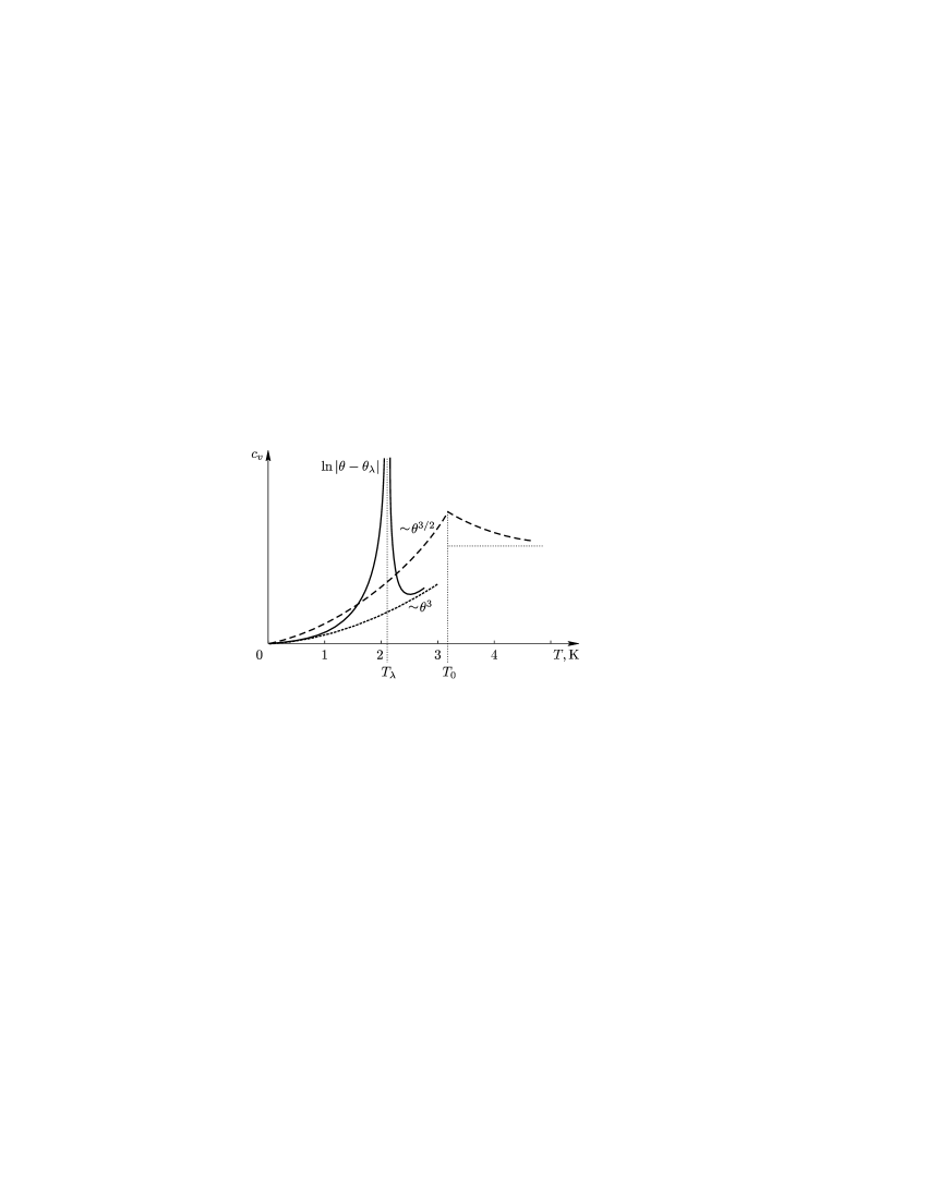
Figure 1: The graph of the heat capacity $c_{v}$ for a quantum Bose gas. In the region of temperatures $0<\theta<1$ on the Kelvin scale, the dependence $c_{v}\sim\theta^{3}$ is typical, and so is the dependence $-\ln|\theta_{\lambda}-\theta|$ in the region of the $\lambda$-point. The graph of the heat capacity of an ideal Bose gas is depicted by the dotted line.

The energy $\cal{E}$ defined at the beginning of Sec. 3 is called global. The quantity $\cal{E}\gg\varepsilon$ is a constant nonstandard number. We studied the $N$-particle Schrödinger equation for symmetric gas molecules interacting in a constant volume $V$ by the Lennard-Jones law (see [15]).

It has turned out that, in the limit, as $N$ (density) increases, the interaction simultaneously decreases, while the energy $\cal{E}\gg\varepsilon$ remains constant, there occurs (under ultrasecond quantization [22] generalizing the Bardeen–Cooper–Schrieffer method for Cooper pairs) a phase transition for $N>N_{\text{cr}}$ from one spectral series [23] to two other series associated with superfluidity (one-dimensional vibrational motion $d=2$ and three-dimensional chaotic vibrational motion $d=6$).

In essence, the particular form of the Lennard-Jones potential in these limit transitions was of no importance; we used only the fact of the existence of a discrete negative (hole) spectrum contributing to the formation of vibrating pairs [24].

Transitions of such type are useful in economic theory, because they are general and are independent of the form of interaction. The transition to the spectrum corresponding to superfluidity is one from chaotic state to joint motion (convection of a gas). A similar situation occurs for flicker noises.

Here the phase transition explains the passage from the individualistic desire to get rich quickly (in Koroviev’s trick, the situation for $k<\sqrt{n}$) to the collective unification with one common aim in mind (convection; in the conjuring trick, the situation for $k\gg\sqrt{n}\ln\ n$). The phase transition to a condensate shows that the cluster individualization of dimers is partially preserved.

In our example of the transition to the condensate state of an ideal Bose gas, there occurs a partial unification into dimers (clusterization) and partial superfluidity. It is the latter phenomenon that leads to the phase transition of zeroth order (the author invoked this transition to explain the so-called spouting effect of Allen and Jones) [31].

Recall that such transitions from one type of energy to other types occur in local spectral series for a fixed constant, but very large global energy $\cal{E}$.

We have regarded the transition to the Bose-condensate state as transition of the kinetic energy of an ideal three-dimensional gas to the vibrational energy of a two-particle ideal (two-point chaotic) gas. The appearance of the $\lambda$-point was interpreted by the author as partial convection, and hence, in view of the momentum conservation law, as one-dimensional vibrational (two-dimensional chaotic) dimension [17]. This explains the two-liquid Thiess–Landau model. A detailed justification of this interpretation was given in [25].

Turbulence was interpreted by the author as transition from the condensate state of a nonchaotic laminary flow to the state of partially chaotic turbulent flow and, therefore, as transition from one type of energy to another type [26], [28].

The Boltzmann equation bewildered mathematicians and physicists by its disagreement with the laws of the classical mechanics of many particles. We explain this discrepancy by the phase transition of the classical condensate (nonchaotic) state to the condensate chaotic one. Only using this approach, can one obtain a rigorous deduction of the Boltzmann equation. The transition to the condensate state yields the solution of the Gibbs paradox problem [21].

One of the important transitions of explosive noise energy is the transition from the potential energy of overhanging snow or rock avalanches to the kinetic energy of moving avalanches, which depends on the random values of the mass and height of the avalanche. The critical value at which this transition can occur, just as that of explosive flicker noise, can be calculated by means of the spectral expansion of the time series.

It is known that both the sociological statistics [29], [30] and animal population statistics correspond to flicker noises.

B.2 On Explosive Flicker Noises

Consider the time series

$$b_{0},b_{1},b_{2},\dots,b_{s},\ \ \sum^{s}_{i=0}b_{i}^{2}\gg 1.$$

Using Kotelnikov’s theorem, we obtain the Fourier series

$$f(t)=\sum_{i=0}^{s}a_{i}\cos\biggl{(}\frac{\pi it}{s}\biggr{)}$$

assuming that the values $b_{j}$,  $j=0,1,\dots,s$, are given at integer points $t=j$. Therefore,

1) $\frac{1}{s}\sum_{i=0}^{s}a_{i}^{2}=\frac{1}{s}\sum^{s}_{i=0}b_{i}^{2}=A_{0}$,  $A_{0}s\gg 1$;

2) the energy $E_{s}$ is

$$E_{s}=\frac{1}{A_{0}}\int_{0}^{2\pi}\biggl{(}\frac{df}{dt}\biggr{)}^{2}(t)\,dt.$$

Hence we have

$$\frac{1}{A_{0}}\sum_{i=0}^{s}i^{2}a^{2}_{i}=\frac{E_{s}s^{2}}{\pi^{2}}.$$ (54)

As is well known, by the spectral density of an interval $l<s$ we mean [36] the mean square of the amplitude; namely,

$$A_{l}=\frac{1}{s-l}\sum_{i=l}^{s}a^{2}_{i}.$$

These definitions can be applied to the case of ordinary noises if take into account their stochastic nature; see, for example, [36].

We have white noise when the spectral density does not decrease. We have a Wiener process when the spectral density decreases as $l^{-2}$,  $s\gg l$.

Here we define explosive flicker noise as noise in the sense of the paper [37] in Secs. 2 and 3.

Let $\cal{E}$ denote the total energy

$${\cal E}=\frac{1}{A_{0}}\sum_{i=0}^{s}i^{2}a_{i}^{2}=\frac{E_{s}s^{2}}{\pi^{2}},\quad s\gg 1.$$ (55)

Definition 1.

By explosive flicker noise we mean a sequence $\{a_{i}^{2}s_{i}\}^{s}_{i=1}$, where the $s_{i}\geq 0$ are integers, such that all the collections $\{a_{i}s_{i}\}^{s}_{i=1}$ are equiprobable under the conditions

$$\sum_{i=0}^{s}s_{i}\leq s,\quad\left[\frac{1}{A_{0}}\sum_{i=0}^{s}a^{2}_{i}s_{i}\right]=s,\quad\frac{1}{A_{0}}\sum_{i=0}^{s}i^{2}a_{i}^{2}s_{i}={\cal E}.$$ (56)

The quantity ${\cal E}$ is called the global energy of explosive flicker noise and $E_{s}$ is its temperature. The process of transition from $s$ to $s+1$ is called an indeterminate process in a sense contrary to the sense of Markov.

Thus, the probability of occurrence of any sequence from the collection $\{a_{i}^{2}s_{i}\}^{s}_{i=1}$ coincides with the probability of occurrence of the sequence $a_{i}^{2},\ i=0,1,2,\dots,s$ satisfying conditions (56). Such a collection $\{a_{i}^{2}s_{i}\}$ is said to be trajectory-probability equivalent to the sequence $a_{i}^{2}$,  $i=0,1,2,\dots,s$.

This means that the input sequence ${a_{i}^{2}}/{A_{0}}$ is a random sample from the given equiprobable collection. This sample is “smooth” in contrast to the other variants of the collection, which “oscillates” about this sample. Only it satisfies the condition on the spectral density (as though it is the weight of the trajectory $s_{i}a_{i}^{2}$,  $i=0,1,2,\dots,s$) Therefore, although we consider “spectral density”, these concepts do not coincide with universally accepted ones, and this fact can lead to a misunderstanding among specialists in the field of random processes. But here we use these concepts in another sense and for special types of noises, namely, explosive flicker noises.

For explosive flicker noises, we present a theorem similar to Theorem 3 from [37]. But, first, let us find the threshold value for $E_{s}$ as a function of $s$. We have

$$\frac{\cal E}{s}=\frac{E_{s}s}{\pi^{2}}\,.$$ (57)

The threshold value for this ratio was, in fact, calculated in Theorems 1-3 from [37], because using the notation $s=N$ in Theorem 2 in that paper or that in Theorems 1 and 3, we obtain ${\cal E}=n$,  $s=k$.

In [37], the critical value $k_{0}$ was calculated as a function of $n$, and if $k_{0}$ is given just as in the above case, then the ratio $n/k$ as a function of $k$ yields the critical value $E_{s}^{\text{cr}}$ as a function of $s$. This is similar to the calculation of the critical temperature for a Bose gas using $N_{\text{cr}}$ [38]. Then Theorem 3 from [37], where $\alpha$ is the rate of decrease of the spectral density, can be carried over to explosive flicker noises in the following form.

Let us define the constants $\beta$ and $\kappa$ from the relations

$$\int_{0}^{\infty}\xi\left(\frac{1}{e^{\beta(\xi+\kappa)}-1}-\frac{s}{e^{\beta s(\xi+\kappa)}-1}\right)d\xi^{\gamma} ={\cal E},$$ (58)

$$\int_{0}^{\infty}\left(\frac{1}{e^{\beta(\xi+\kappa)}-1}-\frac{s}{e^{\beta s(\xi+\kappa)}-1}\right)d\xi^{\gamma} =s,$$ (59)

where $\gamma=1/2-\alpha/4>0$.

Denote

$$c=\int_{0}^{\infty}\left(\frac{1}{\xi}-\frac{1}{e^{\xi}-1}\right)d\xi^{\gamma},\qquad c_{0}=\int_{0}^{\infty}\frac{\xi d\xi^{\gamma}}{e^{\xi}-1}\,.$$

Then

$$E_{s}^{\text{cr}}(\alpha)=\pi^{2}c_{0}c^{-1/\gamma}\beta^{-\gamma},$$ (60)

where $\beta$ is defined from (58) for $\kappa=0$.

Theorem B.1.

1) Let $E_{s}\geq E_{s}^{\text{cr}}(\alpha)$. Let $0<\alpha<2$, and let all the variants $\{s_{i}a_{i}^{2}\}$ satisfying the condition

$$\left[\frac{1}{A_{0}}\sum_{i=0}^{s}a^{2}_{i}s_{i}\right]=s$$

be equiprobable under the condition

$$\frac{1}{A}_{0}\sum_{i=0}^{\infty}|i]^{2}a^{2}_{i}s_{i}={\cal E}.$$

Then the difference

$$\frac{\beta^{\gamma}}{A_{0}}\sum_{i=1}^{s}a^{2}_{i}s_{i}\varphi(\beta i)-\gamma\int_{0}^{\infty}\varphi(x)\frac{1}{|x|^{1-\gamma}}\left\{\frac{1}{e^{x+\kappa}-1}-\frac{s}{e^{s(x+\kappa)}-1}\right\}dx,$$ (61)

where the function $\varphi(x)$ is any bounded piecewise smooth (with finitely many discontinuities) function continuous at the points $\beta i$, tends in probability to zero as $s\to\infty$.

2) Let $E_{s}<E_{s}^{\text{cr}}(\alpha)$. Then, for $s_{0}$, the following ratio holds:

$${\mathbb{P}}\Big{\{}\big{|}s_{0}-\big{[}s-\widetilde{s}(\alpha)\big{]}\big{|}\geq\delta_{1}\widetilde{s}(\alpha)\Big{\}}\leq e^{-|s-\widetilde{s}(\alpha)|^{\gamma/(1+\gamma)}},$$ (62)

where

$$\widetilde{s}(\alpha)=c^{1/\gamma}c_{0}^{1/(1+\gamma)}{\cal E}^{1/(1+\gamma)}$$

and where $\delta$ and $\delta_{1}$ are as small as desired and independent of ${\cal E}$ and $\mathbf{P}$ stands for the ratio of the number of variants satisfying the condition in the brackets to the total number of versions corresponding to the value $s=\widetilde{s}(\alpha)$. For $i<\widetilde{s}(\alpha)+o(\widetilde{s}(\alpha))$, $i<A/\beta$, where $A$ is an arbitrarily large number independent of $\beta$, the following relation holds:

$$\frac{\beta^{\gamma}}{A_{0}}\sum_{i=1}^{[A/\beta]}a_{i}^{2}s_{i}\varphi(\beta i)-\gamma\int_{0}^{\infty}\varphi(x)\frac{1}{|x|^{1-\gamma}}\left\{\frac{1}{e^{x}-1}-\frac{\widetilde{s}(\alpha)}{e^{\widetilde{s}(\alpha)x}-1}\right\}dx\xrightarrow{\mathsf{P}}0\qquad\text{as}\quad s\to\infty.$$

In view of the relation $\sum_{i=o}^{s}s_{i}<s$, this means that $s_{0}$ equal to $s-\widetilde{s}(\alpha)$ occurs in many variants with probability

$$1-\exp\{-|s-\widetilde{s}(\alpha)|^{\gamma/(1+\gamma)-\delta}\}$$.

For $\gamma=0$, we have an analog of Theorem 1 from [37].

The second part of the theorem means an explosive transition to another kind of energy for $s\gg s_{0}(\alpha)$ if the global energy ${\cal E}$ remaind constant, because $s_{0}a_{0}^{2}$ makes no contribution into the global energy of explosive flicker noise (cf. [39]).

This can explain both the transition of turbulent flow (flicker noise according to the Taylor conjecture for Kolmogorov’s law) to laminar flow and the transition of an irreversible process described by the Boltzmann equation and Boltzmann’s $H$-theorem to a fully reversible deterministic process with vanishing entropy governed by the laws of the classical mechanics of many particles.

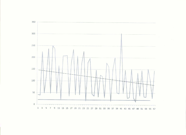
Figure 2: An example of the average money flow. Abscissa axis: days; ordinate axis: average

Eighty years ago, the phenomenon of frequency-proportional fluctuations in electric voltage, i.e., the flickering noise [40], was discovered in electronic devices. In processes with such a spectrum, the energy is pumped from high-frequency to low-frequency fluctuations, and there is a possibility of large-scale catastrophic outbursts. I would not solve this mysterious problem, just as the mysterious problem of the turbulence origination, if I did not notice that the amplitudes of oscillations about the average value of debt flows were tremendous (see Fig. 2). Both problems are in fact equivalent to each other in their mathematical statement.

The transition to turbulence is a phase transition from the Taylor spectrum [40]–[53] to the Kolmogorov spectrum.

References

- [1] P. Lotito, J.-P. Quadrat, and E. Mancinelli, “Traffic assignment and Gibbs–Maslov semirings,” in Idempotent Mathematics and Mathematical Physics, International Workshop, February 3–10, 2003, Vienna, Austria (Amer. Math. Soc., Providence, RI, 2005), pp. 209–219.
- [2] V. A. Dvoryankov, Economic Security: Theory and Possibility of Threats (MO MANPO, Moscow, 2000) [in Russian].
- [3] V. P. Maslov, Quantum Economics, 2nd ed. (Nauka, Moscow, 2006) [in Russian].
- [4] V. P. Maslov, Approximation Probabilities, the Law of Quasistable Markets, and Phase Transitions from the ”Condensed” State, arXiv:math/0307265v1 [math. PR], 19 Jul 2003.
- [5] V. P. Maslov and O. Yu. Shvedov, A Third-Quantized Approach to Large-N Field Models, arXiv:hep-th/9807134.
- [6] V. P. Maslov and O. Yu. Shvedov, Renormalization of the Semiclassical Hamiltonian Field Theory, arXiv:hep-th/9807061.
- [7] V. P. Maslov and O. Yu. Shvedov, Initial Conditions for Semiclassical Field Theory, arXiv:hep-th/9709151.
- [8] V. P. Maslov, “The notions of entropy, Hamiltonian, temperature, and thermodynamical limit in the theory of probabilities used for solving model problems in econophysics,” Russian J. Math. Phys. 9 (4), 437-445 (2002).
- [9] V. P. Maslov and V. E. Nazaikinskii. “On the distribution of integer random variables satisfying two linear relations,” Mat. Zametki 84 (1), 69–98 (2008) [Math. Notes 84 (1–2), 73–99 (2008)].
- [10] P. Erdős, “On some asymptotic formulas in the theory of partitions,” Bull. Amer. Math. Soc. 52, 185–188 (1946).
- [11] A. M. Vershik, “Statistical mechanics of combinatorial partitions, and their limit shapes,” Funktsional. Anal. i Prilozhen. 30 (2), 19–39 (1996) [Functional Anal. Appl. 30 (2), 90–105 (1996)].
- [12] V. P. Maslov and V. V. Vyugin, “Variational problems for additive loss functions and Kolmogorov complexity,” Dokl. Ross. Akad. Nauk 390 (5), 595–598 (2003) [Russian Acad. Sci. Dokl. Math. 67 (3), 404–407 (2003)].
- [13] H. Temperley, “Statistical mechanics and the partition of numbers: I. The transition of liquid helium,” Proceedings of the Royal Society of London. Series A, 199 (1058), 361–375 (1949).
- [14] W. Frish, Turbulence, A. N. Kolmogorov’s Heritage (Fazis, Moscow, 1998) [in Russian].
- [15] V. P. Maslov, “On the Superfluidity of Classical Liquid in Nanotubes: I. Case of even number of neutrons,” Russian J. Math. Phys. 14 (3), 304–318 (2007).
- [16] V. P. Maslov, “On the Superfluidity of Classical Liquid in Nanotubes: III,” Russian J. Math. Phys. 15 (1), 61–65 (2008).
- [17] V. P. Maslov, “Theory of chaos and its application to the crisis of debts and the origin of the inflation,” Russian J. Math. Phys. 16 (1), 103–120 (2009).
- [18] A. Noy, H. Park, et al., “Carbon nanotubes in action,” Nanotoday, 2 (6) (2007).
- [19] S. Joseph and N. Aluru, “Why are carbon nanotubes fast transporters of water?” Nano Letters, 8 (2), 452–458 (2008).
- [20] A. I. Skoulidas, D. M. Ackerman, et al, “Rapid transport of gases in carbon nanotubes,” Physical Review Letters 89 (18), 185901-4 (2002).
- [21] V. P. Maslov, Mathematical Conception of Gas Theory, arXiv:0812.4669, 29 Dec 2008.
- [22] V. P. Maslov, Quantization of Thermodynamics and Ultrasecond Quantization (Institute of Computer Studies, Moscow, 2001) [in Russian].
- [23] V. P. Maslov, “Quasi-Particles Associated with Lagrangian Manifolds Corresponding to Semiclassical Self-Consistent Fields,” Russian J. Math. Phys. 2, 527–534 (1994); 3, 123–132, 271–276, 401–406, 529–534 (1995); 4, 117–122, 265–270, 539–546 (1996); 5, 123–130, 273–278, 405–412, 529–534 (1997/98).
- [24] V. P. Maslov, “New look on the thermodynamics of gas and at the clusterizaton,” Russian J. Math. Phys. 15 (4), 494–511 (2008).
- [25] V. P. Maslov, “On the appearance of the -point in a weakly nonideal Bose gas and the two-liquid Thiess–Landau model” Russian J. Math. Phys. 16 (2), 146–172 (2009).
- [26] V. P. Maslov, “Kolmogorov’s law and the Kolmogorov scales in anisotropic turbulence: the occurrence of turbulence as a result of three-dimensional interaction” Teoret. Mat. Fiz. 94 (13), 386–374 (1993).
- [27] V. P. Maslov, “On the Bose condensate in the two-dimensional case, -point and the Thiess–Landau two-liquid model,” Teoret. Mat. Fiz. 159 (1), 20–23 (2009).
- [28] V. P. Maslov and A. I. Shafarevich, “Rapidly Oscillating Asymptotic Solutions of the Navier-Stokes Equations, Coherent Structures, Fomenko Invariants, Kolmogorov Spectrum, and Flicker Noise,” Russian J. Math. Phys. 13 (4), 414–424 (2006).
- [29] V. P. Maslov, “Modeling of political processes and the role of a person in history,” Sociological Studies, No. 10, 75–82 (2005).
- [30] V. P. Maslov, “Mathematics gives the most precise explanation of the revolution. Solzhenitsyn’s views on the revolution explain very little,” Rossiiskii Kto Est’ Kto [The Russian Who’s Who], No. 3, 15–20 (2007).
- [31] V. P. Maslov, The Economic Law of Increase of Kolmogorov Complexity. Transition from Financial Crisis 2008 to the Zero-Order Phase Transition (Social Explosion), arXiv:0812.4737, 29 Dec 2008.
- [32] V. P. Maslov, “Theorems on the debt crisis and the occurrence of inflation,” Math. Notes 85 (1–2), 146–150 (2009).
- [33] V. P. Maslov, “Gibbs and Bose-Einstein distributions for an ensemble for self-adjoint operators in classical mechanics,” Teoret. Mat. Fiz. 155 (2), 775–779 (2008).
- [34] V. P. Maslov, V. P. Myasnikov, and V. G. Danilov, Mathematical Modeling of the Fourth Accident Block of the Chernobyl Atomic Power Station, (Nauka, Moscow, 1987) [in Russian].
- [35] I. A. Kvasnikov, Thermodynamics and Statistical Physics: Theory of Equilibrium Systems (URSS, Moscow, 2002), Vol. 2 [in Russian].
- [36] G. Shafer and V. Vovk, Probability and Finance. It’s Only a Game!, Wiley Ser. Probab. Stat. Financial Eng. Sect. (Wiley, New York, 2001).
- [37] V. P. Maslov, “Threshold levels in Economics and Time Series,” Math. Notes 85 (5), 305–321 (2009).
- [38] L. D. Landau and E. M. Lifshits, Statistical Physics (Nauka, Moscow, 1964) [in Russian].
- [39] V. P. Koverda and V. N. Skokov, “Statistics of avalanches in stochastic processes with a spectrum,” Physica A 338 (9), 1804–1812 (2009).
- [40] Sh. M. Kogan, Uspehi fiz. nauk, 145 (92), 285–328 (1985) [in Russian].
- [41] V. P. Maslov, Asymptotic Methods for Solving Pseudodifferential Equations, Nauka, Moscow, 1987 [in Russian].
- [42] V. P. Maslov, and G. A. Omel’yanov. Geometric Asymptotics for Nonlinear PDE.I, AMS, Providence, Rhode Island, 2001.
- [43] V. P. Maslov, “Rapidly oscillating solutions of a system of dynamical equations for compressible gas,” Physics of Atmosphere and Ocean, 22 (12), 1253–1254 (1986).
- [44] V. P. Maslov, Resonance Vortexes and Consistent Structures in Turbulent Flow, VINITI, Moscow, 1987 [in English].
- [45] V. P. Maslov and G. A. Omel’yanov, “One-phase asymptotics for equations of magnetohydrodynamics for large Reynolds numbers,” Sibirsk Mat. Zh. 29 (5), 172–180 (1988).
- [46] V. P. Maslov, “Beginning of weakly anisotropic turbulence,” in Proceedings of Symposium on Applied and Industrial Mathematics, Venice, 1989 (Kluver Academic Publ., 1991), 15p.
- [47] V. P. Maslov, “Variation of boundary scale from Kolmogorov to Taylor in turbulent flow in dependence of external noise,” Mat. Zametki 50 (3), 154–158 (1991).
- [48] V. P. Maslov and G. A. Omel’yanov, “Rapidly oscillating solution of magnetohydrodynamics equations in the tokamak approximation,” Teoret. Mat. Fiz. 92 (2), 269–292 (1992).
- [49] V. P. Maslov, G. A. Omel’yanov, and V. A. Tsupin, “Reynolds equations in certain problems of magnetohydrodynamics,” Russian Jour. of Comp. Mechanics 1 (1), (1993).
- [50] V. P. Maslov, “On a new type of turbulence for incompressible magnetohydrodynamics,” in Turbulence in Fluid Flows; A Dynamical Systems Approach, Ed. by G. R. Sell, C. Foias, R. Temam; Ser. The IMA Volumes in Mathematics and its Applications, vol. 55; pp. 87–100.
- [51] V. P. Maslov, “Kolmogorov law and Kolmogorov scales in anisotropic turbulence. Beginning of turbulence because of three-scale interaction,” Teoret. Mat. Phys. 94 (3), 368–374 (1993).
- [52] V. P. Maslov and G. A. Omel’yanov, “Three-scale expansion of solutions of MHD equations and the Reynolds equation for tokamak,” Teoret. Mat. Phys. 98 (2), 397–411 (1994).
- [53] V. P. Maslov and G. A. Omel’yanov, “Turbulent bending of plasma pinch in a vacuum,” Dokl. Ross. Akad. Nauk 336 (3), 320–323 (1994).