Neuronal coding of pacemaker neurons – A random dynamical systems approach

Abstract

The behaviour of neurons under the influence of periodic external input has been modelled very successfully by circle maps. The aim of this note is to extend certain aspects of this analysis to a much more general class of forcing processes. We apply results on the fibred rotation number of randomly forced circle maps to show the uniqueness of the asymptotic firing frequency of ergodically forced pacemaker neurons. The details of the analysis are carried out for the forced leaky integrate-and-fire model, but the results should also remain valid for a large class of further models.

1 Introduction

Already in 1907, long before the molecular mechanisms of neural signal transduction had been clarified, Louis Lapicque proposed a simple model for the firing behaviour of a neuron [2, 3, 4]. A crucial feature of this so-called integrate-and-fire model (IFM) is the separation of time-scales: the stereotypical and extremely fast generation of an action potential is thought of as being concentrated in a single moment of time, whereas the much slower evolution of the membrane potential in the interspike intervals is modelled as a continuous process. For many questions concerning the behaviour of neural systems this level of abstraction turned out to be exactly the adequate one, such that even nowadays, more than a hundred years after Lapicque’s original paper, the different variations of the IFM still play a central role in theoretical neuroscience [5]. One of their great achievements was the explanation of so-called ‘paradoxical segments’ that were discovered in the experimental investigation of pacemaker neurons in the nervous system of crayfish (Procambarus clarkii), sea slugs (Aplysia californica) and horseshoe crabs (Limulus polyphemus) [6, 7]. The counter-intuitive observation that was made in these experiments was that an increase in the frequency of periodic inhibitory presynaptic input can lead to an increase of the post-synaptic firing frequency. This paradoxon was explained by relating the respective theoretical models to monotone circle maps whose rotation number equals the ratio between the input and the output frequency. When the circle map has a stable periodic orbit, then input and output frequency remain directly proportional on a small neighbourhood (the paradoxical segment), disrespective of whether the input is inhibitory or excitatory [6, 8, 9, 10] (see also Section 2). Similar ideas have also been pioneered before by V. Arnold in the study of cardiac cells [11, 12].

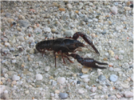
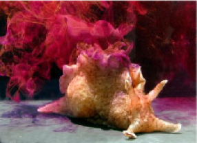
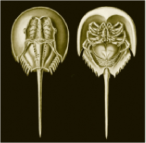
Figure 1.1: Three species for which mode-locking phenomena in the nervous system have been investigated experimentally [6, 7]. From left to right: Procambarus clarkii, Aplysia californica and Limulus polyphemus [13].

It must be said, however, that despite the great success of IFMs and the long history of their investigation their rigorous mathematical description is still restricted to a few very special situations. In particular, the only types of external forcing that can be treated analytically so far are either periodic [14, 15] or stationary stochastic input [16, 17, 18]. Even the superposition of the two – noisy periodic input – is mostly accessible only by numerical methods [19]. Our goal here is take up the ideas used in the analysis of the periodically forced IFM an to extend these to more general forcing processes. Thereby, we restrict ourselves to deterministic and/or random forcing, although it should be possible to adapt the approach to models generated by stochastic differential equations as well. In order to state the main results, we first recall the construction of the IFM.

The membrane potential $V(t)$ of a neuron ${\cal N}_{1}$ remains between a lower threshold $V_{l}$ and an upper threshold $V_{u}$. $V(t)$ can never drop below $V_{l}$ due to physiological constraints, whereas when it reaches $V_{u}$ the neuron ‘fires’, meaning that an action potential is triggered and $V(t)$ drops back to a rest potential $V_{r}\in[V_{l},V_{u})$. Between the two thresholds, the potential evolves according to an infinitesimal law

(1.1) $$\dot{V}(t)\ =\ F(t,V(t))\$$

with right side $F:\mathbb{R}^{2}\to\mathbb{R}$ that should satisfy $F(t,V_{l})\geq 0\ \forall t\in\mathbb{R}$. The dependence of $F$ on $t$ corresponds to the influence of external time-dependent factors. The reset procedure when $V(t)$ reaches $V_{u}$ is usually expressed as

(1.2) $$V(t^{+})\ =\ V_{r}\quad\textrm{ if }V(t)=V_{u}\ ,$$

where $t^{+}$ denotes the right-hand limit. Identifying the interval $[V_{l},V_{u})$ with the circle $\mathbb{T}^{1}=\mathbb{R}/\mathbb{Z}$, this gives rise to a non-autonomous circle flow (see Figure 1.1).

For fixed initial values $V(t_{0})=x_{0}$, we denote by $t_{n}$ the time of the $n$-th firing of the neuron ${\cal N}_{1}$. Then a very basic and fundamental question is that of the existence and uniqueness of the asymptotic firing frequency: under what assumptions does the limit

(1.3) $$\nu_{{\cal N}_{1}}\ =\ \lim_{n\rightarrow\infty}n/t_{n}\$$

exist and when is it independent of the initial values $t_{0}$ and $x_{0}$?

Figure 1.2: Construction of the potential flow $V(t)$ generated by (1.1) and (1.2) with initial values $V(t_{0})=x_{0}$.

In the simplest case the external input is periodic in time with period $p\in\mathbb{R}^{+}$. As mentioned, this situation is quite well-understood and has been studied for a number of different versions of the IFM [14, 15]. The analysis depends on the choice of a suitable Poincaré section for the flow, by which one obtains a circle map $g:\mathbb{T}^{1}\to\mathbb{T}^{1}$ whose lift $G:\mathbb{R}\to\mathbb{R}$ generates the rescaled sequence $t_{n}$, that is $t_{n+1}/p=G^{n}(t_{n}/p)$. (We briefly recall the construction in Section 2.) Under suitable assumptions on the function $F$ this map $g$ has good monotonicity properties that ensure the existence and uniqueness of the rotation number

(1.4) $$\rho(G)\ =\ \lim_{n\rightarrow\infty}G^{n}(t_{0}/p)/n\ =\ \nu_{{\cal N}_{1}}^{-1}/p$$

and thus of the asymptotic firing frequency. As indicated above, the existence of a stable periodic orbit for the map $g$ yields an explanation for the ‘paradoxical segments’ in situations with inhibitory presynaptic input.

A good framework to study more general forcing processes is provided by the theory of random dynamical systems, as exposed in [20]. In order to model the external input we will assume that there is an underlying forcing process, given by a measure-preserving or metric dynamical system (metric DS), that is, a quadruple $(\Theta,{\cal B},\mu,\omega)$ where $(\Theta,{\cal B},\mu)$ is a probability space and $\omega:\mathbb{R}\times\Theta\to\Theta,(t,\theta)\mapsto\omega_{t}(\theta)$ and $\omega$ is a flow on $\Theta$ that leaves the probability measure $\mu$ invariant (compare [20]). We usually write $\omega_{t}(\theta)=\theta\cdot t$. In this setting (1.1) is replaced by

(1.5) $$\dot{V}(t)\ =\ F(\theta_{0}\cdot t,V(t))$$

where $F:\Theta\times\mathbb{R}\to\mathbb{R}$ and $\theta_{0}$ is some initial value in $\Theta$. In order to ensure that (1.5) generates a RDS, we have to impose some standard technical conditions on $F$. We say $F$ is uniformly Lipschitz-continuous in $V$ if there exists a constant $L>0$ such that

(1.6) $$|F(\theta,V)-F(\theta,V^{\prime})|\ \leq\ L\cdot|V-V^{\prime}|\quad\forall\theta\in\Theta,\ V,V^{\prime}\in\mathbb{R}\ .$$

For the moment, we will just assume that $F$ is bounded and uniformly Lipschitz-continuous in $V$. These assumptions seem quite reasonable from the physiological point of view. It is also possible to weaken them further to some extent and we will discuss this issue in detail at the beginning of Section 4.

Due to the lack of a suitable structure on $\Theta$, it is not feasible anymore to take a Poincaré section in this situation. However, it turns out that instead the flow generated by (1.2) and (1.5) can be analysed directly by applying a result on the fibred rotation number of randomly forced circle flows. (Basically, what we need is a slight modification of statements from [21] that we present in Section 3.) This leads to the following result.

Theorem 1.1.

Suppose that the metric DS $(\Theta,{\cal B},\mu,\omega)$ is ergodic and the function $F$ in (1.5) is bounded on $\Theta\times[0,1]$ and uniformly Lipschitz-continuous and non-increasing in $V$. Then the model described by (1.2) and (1.5) has a unique asymptotic firing frequency in the following sense: There exists a real number $\nu$ such that for $\mu$-almost every $\theta_{0}\in\Theta$ and all $x_{0}\in[V_{l},V_{r})$ there holds

(1.7) $$\lim_{n\rightarrow\infty}n/t_{n}\ =\ \nu\ .$$

A well-known example to which this statement applies is the leaky integrate-and-fire model (LIFM), in which the function $F$ takes the form

(1.8) $$F(\theta,V)\ =\ -a(\theta)\cdot V+b(\theta)\ .$$

Here $a:\Theta\to\mathbb{R}^{+}$ corresponds to the membrane permeability whereas $b:\Theta\to\mathbb{R}$ reflects the external input. In order to apply Theorem 1.1 we have to assume that $a$ and $b$ are bounded. Slightly weaker conditions are again discussed at the beginning of Section 3. The LIFM was first introduced by Stein [8] and then further investigated both theoretically and experimentally by Knight [9, 7]. In contrast to the so-called ‘perfect integrator’ or ‘perfect IFM’ ($\frac{\partial}{\partial V}F\equiv 0$) with ‘infinite memory’ used by Lapicque, it takes into account the exponential decay of the membrane depolarisation in time after excitation.

The most subtle issue in the proof of Theorem 1.1 is the fact that when $F$ takes negative values, then this might lead to discontinuities in the flow $V(t)$ and to a lack of monotonicity with respect to the initial condition $x_{0}$ (see Figure 2.1). At this point, the monotonicity of $F$ in $V$ is needed in order to recover a certain ‘almost-monotonicity’ property. The discontinuity does not present a problem in the setting of RDS, but impedes drawing further conclusions in the situation where the base flow $\omega$ is a uniquely ergodic system on a compact metric space $\Theta$. All these complications can be avoided by assuming that $F$ is non-negative. In this case, we have the following.

Theorem 1.2.

Suppose that the metric DS $(\Theta,{\cal B},\mu,\omega)$ is ergodic and the function $F$ in (1.5) is bounded on $\Theta\times[0,1]$, uniformly Lipschitz-continuous in $V$ and $F(\theta,V_{r})>0\ \forall\theta\in\Theta$. Then the following holds.

• The model described by (1.2) and (1.5) has a unique asymptotic firing frequency: There exists a real number $\nu$ such that for $\mu$-almost every $\theta_{0}\in\Theta$ and all $x_{0}\in[V_{l},V_{u})$ there holds

  (1.9) $$\lim_{n\rightarrow\infty}t_{n}/n\ =\ \nu\ .$$

• If in addition $\Theta$ is a compact metric space, $F$ is continuous, $F(\theta,V_{u})>0\ \forall\theta\in\Theta$ and $\omega$ is uniquely ergodic, then (1.9) holds for all initial conditions $(\theta_{0},x_{0})\in\Theta\times[V_{l},V_{u})$ and the convergence is uniform in $(\theta_{0},x_{0})$.

This statement can, for instance, be applied to the so-called quadratic IFM, which is given by (1.2) and (1.5) with

(1.10) $$F(\theta,V)\ =\ V^{2}+I(\theta)\ ,$$

under the additional assumption that $\inf_{\theta\in\Theta}I(\theta)>\max\{-V_{r}^{2},-V_{u}^{2}\}$. (See [15] for the analysis of this model in the periodically forced case and further references). The standard example of a uniquely ergodic base flow would be the Kronecker flow $\theta\cdot t=\theta+t(\omega_{1},\ldots,\omega_{d})$ with $d$ rationally independent frequencies $\omega_{1},\ldots,\omega_{d}$, corresponding to the excitation of ${\cal N}_{1}$ by $d$ independent pacemaker neurons. Although we will not discuss the topic in detail, we want to mention that mode-locking phenomena may appear in this setting whenever the asymptotic firing frequency is rationally related to the driving frequencies $(\omega_{1},\ldots,\omega_{d})$

Acknowledgments. The author would like to thank K. Pakdaman for interesting discussions that initiated this research. This work was supported by a research fellowship (Ja 1721/1-1) of the German Research Council (DFG).

2 Periodic forcing revisited

In this section we briefly recall the analysis of the periodically forced IFM and in particular the construction of the circle map $g$ mentioned in the introduction. This will also allow to discuss the modifications needed to extend the approach to randomly forced models. In order to simplify notation, we will from now on always assume that $V_{l}=0$ and $V_{u}=1$.

Suppose that the function $F$ in (1.1) is $p$-periodic in the second variable, that is

(2.1) $$F(t,V+p)\ =\ F(t,V)\ .$$

Equivalently, we may assume that $\Theta=\mathbb{T}^{1}$ and $\omega_{t}(\theta)=\theta+t/p\bmod 1$ in (1.5). For simplicity, we also suppose that

(2.2) $$F(t,V_{r})\ >\ 0\quad\forall t\in\mathbb{R}\ .$$

In this case, we may assume without loss of generality that $V_{r}=V_{l}=0$, since the interval $(V_{l},V_{r})$ is not accessible from outside and does not play a role in the description of the dynamics. The ODE (1.1) generates a flow

(2.3) $$\Phi\ :\quad\mathbb{R}^{2}\to\mathbb{R}\ ,\quad(t,V)\mapsto\Phi_{t}(V)$$

in the sense that $x(t)=\Phi_{t-t_{0}}(x_{0})$ is the solution of (1.1) with initial conditions $x(t_{0})=x_{0}$. The first firing time $t_{1}$ can then be expressed as $t_{1}=t_{0}+\inf\{t\geq 0\mid\Phi_{t-t_{0}}(x_{0})=1\}$. Fixing the initial value $x_{0}=V_{r}$, this allows to define a map $\tilde{G}:\mathbb{R}\to\mathbb{R},\ t_{0}\mapsto t_{1}$ that generates the sequence of spiking times $t_{n}$, that is, $t_{n+1}=\tilde{G}(t_{n})\ \forall n\in\mathbb{N}_{0}$. Rescaling $\tilde{G}$, we let $G:\mathbb{T}^{1}\to\mathbb{T}^{1},\ x\mapsto G(pt)/p$. The periodicity assumption (2.1) implies that $\tilde{G}(t+p)=\tilde{G}(t)+p$ and therefore $G(t+1)=G(t)+1$. Consequently $G$ is the lift of a circle map $g:\mathbb{T}^{1}\to\mathbb{T}^{1}$. Furthermore, using (2.2) it is possible to show the map $G$ is continuous and strictly monotonically increasing, such that $g$ is an orientation-preserving circle homeomorphism. Such maps have a well-defined rotation number defined by the limit

(2.4) $$\rho(G)\ =\ \lim_{n\rightarrow\infty}(G^{n}(t)-t)/n\ =\ \lim_{n\rightarrow\infty}(\tilde{G}^{n}(pt)/p-pt)/pn$$

which always exists and is independent of $t$ (see, for example, [23]). Of course, this immediately implies the existence and uniqueness of the asymptotic firing frequency $\nu_{{\cal N}_{1}}=\frac{1}{p}\cdot\rho(\tilde{G})^{-1}$.

There is also an alternative way of constructing the map $g$ that yields some additional insight and which we want to discuss on an informal level. Suppose we let

(2.5) $$\tilde{F}\ :\mathbb{R}^{2}\to\mathbb{R}^{2}\ ,\quad(y,V)\mapsto(1/p,F(py,V-n))\quad\textrm{ if }V\in[n,n+1)\ .$$

Then $\tilde{F}$ defines a vector field on $\mathbb{R}^{2}$ that is invariant under integer translations and hence projects to a vector field on the two-torus $\mathbb{T}^{2}$. Consequently, the flow $\tilde{\Psi}:\mathbb{R}\times\mathbb{R}^{2}\to\mathbb{R}^{2}$ generated by $\dot{Y}(t)=F(Y(t)),\ Y\in\mathbb{R}^{2}$, projects to a flow $\Psi$ on $\mathbb{T}^{2}$. It is now easy to see that the map $g$ defined above is simply the return map of $\Psi$ to the Poincaré section $\mathbb{T}^{1}\times\{0\}$. (Note that (2.2) ensures that this section is transversal to the flow direction.) However, from this point of view we also see that taking this particular Poincaré section has something arbitrary. For example, one might just as well have chosen to define another circle homeomorphism $\hat{g}$ with lift $\hat{G}:\mathbb{R}\to\mathbb{R}$ by taking the Poincaré map of the vertical section $\{0\}\times\mathbb{T}^{1}$. This simply corresponds to stopping the flow at times $\hat{t}_{n}=np$. The asymptotic firing frequency could thus be obtained as $\nu_{{\cal N}_{1}}=\rho(\hat{G})/p$. One can even arrive at the same conclusion without resort to Poincaré sections at all. As $\tilde{F}$ is constant in the first coordinate, the flow $\Psi$ has skew product structure over the simple base flow $\omega_{t}(t_{0})=t_{0}+t/p\ \bmod 1$. In other words, $\Psi$ is a periodically forced circle flow with lift $\tilde{\Psi}$. As circle homeomorphisms, such flows have a well-defined vertical rotation number and one obtains $\nu_{{\cal N}_{1}}=\rho(\tilde{\Psi})/p=\lim_{t\to\infty}\pi_{2}\circ\tilde{\Psi}_{t}(t_{0},x_{0})$.

Now, in the case of periodic forcing all this is surely a mere tautology. However, things become quite different as soon as one wants to consider more general types of forcing. When the driving space $\Theta$ is an arbitrary measurable space, then taking a vertical Poincaré section does not make sense anymore, whereas the Poincaré return map to $\Theta\times\{0\}$ just yields a self-map of $\Theta$ that might be very difficult to analyse. In this context, the fact that we can also directly consider the forced circle flow $\Psi$ generated by (1.2) and (1.5) turns out to be a great advantage. In the next section, we will present a result on randomly forced circle flows and their lifts that ensures the existence and uniqueness of the vertical or fibred rotation number of such skew product flows. The remaining sections are then dedicated to the construction of suitable lifts for the potential flow in the situation of Theorems 1.1 and 1.2, which immediately leads to proofs of the respective statements.

Finally, before turning to the rigorous analysis in the next sections, we briefly want to indicate why further technical problems appear when condition (2.2) does not hold anymore. First of all, this evidently leads to discontinuities of the flow when the potential ‘jumps’ from $V_{u}=1$ to $V_{r}\in(0,1)$ or, when considering lifts, from $V_{u}+n$ to $V_{r}+n+1$ for some $n\in\mathbb{Z}$. This would in itself not present a serious problem, since most results on the existence and uniqueness of rotation numbers only require monotonicity, whereas continuity is less important. However, it turns out that dropping condition (2.2) may at the same time lead to a lack of monotonicity of the circle flow. An example of how this can happen is indicated in Figure . This remains true even when $F$ is non-increasing in $V$, as assumed in Theorem 1.1. However, in this situation it is nevertheless possible to make the argument work. In the case of periodic forcing, one can show that lift $G$ of the circle map $g$ constructed above is monotonically increasing on the image of one of its iterates (as done in [14, 15]). On the level of forced flows, one may similarly show that while two different orbits may reverse their order, they will always remain within a bounded distance of each other. (This is the point of view we will adopt in Section 5.) In both cases, this is still sufficient to guarantee the existence and uniqueness of the rotation number.

Figure 2.1: Lack of monotonicity of the lift of the potential flow. Two solutions $V_{1}(t)$ and $V_{2}(t)$ with $V_{1}(t_{0})=x_{1}<x_{2}=V_{2}(t_{0})$ have changed order at time $s$.

3 Uniqueness of the fibred rotation number

As mentioned before, we say $(\Theta,{\cal B},\mu,\omega)$ is a metric DS if $(\Theta,{\cal B},\mu)$ is a probability space and $\omega:\mathbb{R}\times\Theta\to\Theta,\ (t,\theta)\mapsto\omega_{t}(\theta)$ is a flow that preserves $\mu$, meaning that $\mu\circ\omega_{t}^{-1}=\mu\ \forall t\in\mathbb{R}$. As before, we write $\omega_{t}(\theta)=\theta\cdot t$. A random dynamical system (RDS) over $\omega$ is a measurable mapping

(3.1) $$\Psi\ :\quad\mathbb{R}\times\Theta\times\mathbb{R}\to\Theta\times\mathbb{R}\ ,\quad(t,\theta,x)\mapsto(\theta\cdot t,\psi_{t}(\theta,x))$$

that satisfies the cocycle property

(3.2) $$\psi_{t_{1}+t_{2}}(\theta,x)\ =\ \psi_{t_{2}}(\theta\cdot t_{1},\psi_{t_{1}}(\theta,x))\quad\forall(t_{1},t_{2},\theta,x)\in\mathbb{R}^{2}\times\Theta\times\mathbb{R}\ .$$

We say $\Psi$ is a continuous RDS if for all $\theta\in\Theta$ the mapping $(t,x)\mapsto\psi_{t}(\theta,x)$ is continuous.

Evidently, what we are interested in is the existence of uniqueness of the fibred rotation number

(3.3) $$\rho(\Psi)\ =\ \lim_{t\to\infty}(\psi_{t}(\theta,x)-x)/t\$$

when $\Psi$ is obtained as the lift of a randomly forced circle flow. For this, we will use the following assumptions:

• There holds

  (3.4) $$\psi_{t}(\theta,x+1)\ =\ \psi_{t}(\theta,x)+1\quad\forall(t,\theta,x)\in\mathbb{T}\times\Theta\times\mathbb{R}\ .$$

  In particular, this implies that $\Psi$ projects to a random dynamical system on the circle $\mathbb{T}^{1}$.

• There exists a constant $C\geq 0$ such that

  (3.5) $$\psi_{t}(\theta,x)\ \leq\ \psi_{t}(\theta,x^{\prime})+C\quad\forall(t,\theta,x,x^{\prime})\in\mathbb{T}\mathbb{T}^{1}\Theta\times\mathbb{R}^{2}\textrm{ with }x\leq x^{\prime}\ .$$

  In other words, the mappings $\psi_{t}(\theta,\textbf{.})$ are ‘almost monotone’ in $x$, up to a uniform constant $C$.

• There exists a constant $\eta\geq 0$ such that

  (3.6) $$|\psi_{t}(\theta,x)-x|\ \leq\ \eta\quad\forall(t,\theta,x)\in[0,1]\times\Theta\times\mathbb{R}\ .$$

Theorem 3.1.

Suppose that $(\Theta,{\cal B},\mu,\omega)$ is ergodic and the RDS $\Psi$ satisfies (3.4)–(3.6). Then there exists a real number $\rho$ and a set $\Theta_{0}\subseteq\Theta$ of full measure, such that

(3.7) $$\lim_{t\to\infty}(\psi(t,\theta,x)-x)/t\ =\ \rho\quad\forall(\theta,x)\in\Theta_{0}\times\mathbb{R}\ .$$

Remark 3.2.

• When $\Theta$ is a compact metric space and $\omega$ a uniquely ergodic flow on $\Theta$, then this result is well-known and due to Herman [24]. (See also [25] for a precursor in the context of quasiperiodic Schrödinger operators.) For the more general case of ergodically forced monotone circle maps, it was proved more recently by Li and Lu [21]. The only new aspect here is that we work with continuous time replace monotonicity by the slightly weaker property (3.5). It is not surprising that this can be proved along the same lines as the previous results, but since the proof is rather short anyway we include the details for the convenience of the reader.

• When $\Psi$ is a continuous RDS on the circle, then assumption (3.5) can be replaced by the much more general one that

  (3.8) $$\lim_{t\to\infty}|\psi_{t}(\theta,x)-\psi_{t}(\theta,x^{\prime})|/t\ =\ 0\quad\forall(\theta,x,x^{\prime})\in\Theta\times\mathbb{R}^{2}\ .$$

  In this case Herman’s original proof, which uses the existence of a $\Psi$-invariant probability measure that projects down to $\mu$, remains valid with hardly any modifications. However, since we do not assume $\Psi$ to be continuous (and this is crucial for the application to the forced LIFM), such an invariant measure does not necessarily exist.

Proof of Theorem 3.1. By (3.4) and (3.5) we have

(3.9) $$|(\psi_{t}(\theta,x)-x)-(\psi_{t}(\theta,x^{\prime})-x^{\prime})|\ \leq\ C+1\quad\forall(t,\theta)\in\mathbb{T}\times\Theta,x,x^{\prime}\in A_{\theta}\ .$$

(Note that due to (3.4) we may assume w.l.o.g. that $x\in[x^{\prime}-1,x^{\prime})$), in which case the estimate is a direct consequence of (3.5).) It follows that when the limit $\rho(\theta,x):=\lim_{t\to\infty}(\psi_{t}(\theta,x)-x)/t$ exists for one $x\in\mathbb{R}$, it exists for all $x\in\mathbb{R}$ and does not depend on $x$. Given any $n\in\mathbb{N}_{0}$, let $F_{n}(\theta):=\psi_{n}(\theta,0)+C+1$. Then (3.9) implies that

$$F_{n+m}(\theta) = \psi_{n+m}(\theta,0)+C+1\ =\ \psi_{m}(\theta\cdot n,\psi_{n}(\theta,0))-\psi_{n}(\theta,0)+F_{n}(\theta)$$

$$\stackrel{{\scriptstyle(\ref{eq:4})}}{{\leq}} \psi_{m}(\theta\cdot n,0)+C+1+F_{n}(\theta)\ =\ F_{m}(\theta\cdot n)+F_{n}(\theta)\ .$$

Thus the random variables $F_{n}$ form a subadditive sequence over the measure-preserving transformation $\theta\mapsto\theta\cdot 1$. Further (3.6) implies that $F_{1}$ is bounded. Hence, we can apply Kingman’s Subadditive Ergodic Theorem (see, for example, [20]), which yields the existence of a $\mu$-integrable function $\tilde{\rho}:\Theta\to\mathbb{R}$ and a set $\Theta^{\prime}\subseteq\Theta$, such that for all $\theta\in\Theta^{\prime}$ there holds

$$\lim_{n\rightarrow\infty}F_{n}(\theta)/n\ =\ \tilde{\rho}(\theta)\ .$$

(3.6) and (3.9) together now now imply that for all $(\theta,x)\in\Theta^{\prime}\times\mathbb{R}$ we have

$$\lim_{t\to\infty}(\psi_{t}(\theta,x)-x)/t\ =\ \tilde{\rho}(\theta)\ .$$

It is easy to see that the function $\tilde{\rho}$ is invariant, that is $\tilde{\rho}(\theta\cdot t)=\tilde{\rho}(\theta)\ \forall t\in\mathbb{T}$, and the ergodicity of the base flow $\omega$ therefore implies that $\tilde{\rho}(\theta)=\int_{\Theta}\tilde{\rho}\ d\mu=:\rho$ on a set of full measure $\Theta^{\prime\prime}$. If we now let $\Theta_{0}=\Theta^{\prime}\cap\Theta^{\prime\prime}$ then all the assertions of the theorem are satisfied. ∎

4 Construction of the potential flow

The aim of this section is to formalise the model described by (1.2) and (1.5) in the introduction and to prove Theorem 1.2. (The proof of Theorem 1.1 will then be given in Section 5.) More precisely, we will construct a lift $\widehat{V}$ for the circle flow $V$ that describes the evolution of the membrane potential (recall that we identify the interval $[V_{l},V_{u})$ with the circle. We assume without loss of generality that $V_{l}=0$ and $V_{u}=1$. Unfortunately, the construction has a somewhat technical flavour, which basically comes from the need to treat the discontinuities produced by (1.2) in a formally precise way. However, in order to treat the problem in a rigorous way a certain amount of detail seems unavoidable, in particular since the ‘almost-monotonicity property’ needed for the proof of Theorem 1.1 is a rather subtle issue.

Suppose that $(\Theta,{\cal B},\mu,\omega)$ is a metric DS and consider the non-autonomous differential equation

(4.1) $$\dot{x}(t)\ =\ F(\theta\cdot t,x(t))$$

with $F:\mathbb{R}\times\Theta\to\mathbb{R}$, which is equivalent to (1.5). As mentioned in the introduction, we first discuss the precise technical conditions on $F$ needed for the construction. Given any $f:\mathbb{R}\to\mathbb{R}$, we let

$$\|f\|_{[0,1],0,0} = \sup_{x\in[0,1]}|f(x)|\quad\textrm{ and }$$

$$\|f\|_{[0,1],0,1} = \|f\|_{[0,1],0,0}+\sup_{x\neq y\in[0,1]}\frac{|f(y)-f(x)|}{|y-x|}\ .$$

(The terminology follows [20, Appendix B].) We then require that there exists a constant $C>0$, such that for all $\theta\in\Theta$ there holds

(4.2) $$\int_{0}^{1}\|F(\theta\cdot t,\textbf{.})\|_{[0,1],0,0}\ dt \leq C\quad\textrm{ and }$$

(4.3) $$\int_{0}^{1}\|F(\theta\cdot t,\textbf{.})\|_{[0,1],0,1}\ dt < \infty\ .$$

The restriction to the interval $[0,1]$ in the definition of the norms is explained by the fact that due to the reset procedure described by (1.2) this is the only part of the phase space we are interested in. We could equally assume that the conditions are satisfied on all of $\mathbb{R}$ and just modify the function $F$ if they are violated outside of $[0,1]$. Assumption (4.2) is needed to ensure that the hypothesis of Theorem 3.1 in the appendix are met – roughly spoken, it just ensures that action potentials or spikes cannot be generated at an arbitrary rate (there will be at most $C/(1-V_{r})+1$ spikes in any interval of length 1). (4.3) is just a standard technical condition which ensures that (4.1) generates a RDS

(4.4) $$\Phi\ :\quad\mathbb{R}\times\Theta\times\mathbb{R}\ \to\Theta\times\mathbb{R}\ ,\quad\Phi(t,\theta,x)=(\theta\cdot t,\varphi_{t}(\theta,x))$$

over the base flow $\omega$ (see [20, Theorem 2.2.2]). From now on, we will always assume that $\Phi$ is the skew product flow generated by (4.1).

In the following, we will give a precise definition of the lift of the potential semiflow

(4.5) $$\widehat{V}\ :\quad\mathbb{R}^{+}\times\Theta\times\mathbb{R}\ ,\quad(t,\theta,v)\mapsto(\theta\cdot t,\widehat{V}_{t}(\theta,x))\$$

corresponding to the model described by (1.2) and (1.5). The membrane potential at time $t$ with initial values $t=0$, $\theta$ and $x_{0}$ is then obtained as $V(t)=\widehat{V}_{t}(\theta,x_{0})\bmod 1$. The only assumption on $F$ needed for this construction is (4.3). (4.2) and the additional assumptions made in Theorems 1.1 and 1.2 will be required only later in order to ensure that $\widehat{V}$ meets the assumptions of Theorem 3.1.

Given any $x\in\mathbb{R}$, we denote by $[x]\in\mathbb{Z}$ its integer part and by $\{x\}=x-[x]\in[0,1)$ its fractional part. For any $(\theta,x)\in\Theta\times\mathbb{R}$ we define

(4.6) $$\tau(\theta,x)\ =\ \inf\left\{t\geq 0\mid\varphi_{t}(\theta,\{x\})=1\right\}\$$

with $\tau(\theta,x)=\infty$ if the set on the right is empty. This is the time when the first spike is generated.

For any $s\in(\mathbb{R}^{+})^{\mathbb{N}}$ we denote by $S=S(s)$ the sequence given by $S_{n}=\sum_{i=0}^{n}s_{i}$. Then, given $(\theta,x)\in\Theta\times\mathbb{R}$, we recursively define a sequence $s_{n}=s_{n}(\theta,x)$ and the corresponding sequence $S_{n}=S_{n}(\theta)$ by

(4.7) $$s_{0}=0\ ,\ s_{1}=\tau(\theta,x)\quad\textrm{and}\quad s_{n+1}=\tau(\theta\cdot S_{n},V_{r})\ .$$

(Recall that $V_{r}\in[0,1)=[V_{l},V_{u})$ is the rest potential introduced in (1.2).) $S_{n}$ is the time when the $n$-th action potential is triggered, whereas $s_{n}$ is the length of the time interval between the $n-1$-th and the $n$-th spike. Given $(t,\theta,x)\in\mathbb{R}^{+}\times\Theta\times\mathbb{R}$ we define $n(t,\theta,x)$ as the unique integer $n$ such that $S_{n}(\theta,x)\leq t<S_{n+1}(\theta,x)$, that is

(4.8) $$n(t,\theta,x)\ =\ \max\{n\in\mathbb{N}\mid S_{n}(\theta,x)\leq t\}\ .$$

In other words, $n(t,\theta,x)$ is just the number of spikes generated until time $t$. The lifted potential flow is then defined by (4.5) with

(4.9) $$\widehat{V}_{t}(\theta,x)\ =\ \left\{\begin{array}[]{ll}[x]+\varphi_{t}(\theta,\{x\})&\textrm{if }n(t,\theta,x)=0\ ;\\ \\ {[}x]+n+\varphi_{t-S_{n}}(\theta\cdot S_{n},V_{r})&\textrm{if }n(t,\theta,x)=n\ .\end{array}\right.$$

Remark 4.1.

• The circle flow $V$ defined by (1.2) and (1.5) is typically not continuous and therefore a priori has many different lifts that do not only differ by an integer constant. However, the particular lift $\widehat{V}$ defined above is the unique one that ‘counts’ the number $n(t,\theta,x)$ of spikes (action potentials) generated up to time $t$, in the sense that $n(t,\theta,x)$ equals the number of integers in the interval $[x,\widehat{V}_{t}(\theta,x)]$. In this way, the asymptotic firing frequency is obtained as the inverse of the rotation number

  (4.10) $$\rho(\widehat{V})\ =\ \lim_{t\to\infty}(\widehat{V}_{t}(\theta,x))/t\ ,$$

  provided this limit exists. To show that this is the case under the assumptions made in Theorem 1.2 is the aim of the remainder of this section.

• We note that

  (4.11) $$\widehat{V}_{t}(\theta,x+1)\ =\ \widehat{V}_{t}(\theta,x)+1\quad\forall(t,\theta,x)\in\mathbb{R}^{+}\times\Theta\times\mathbb{R}\ .$$

  Further, when (4.2) holds then

  (4.12) $$|\widehat{V}_{t}(\theta,x)-x|\ \leq\ \frac{C}{1-V_{r}}+1\quad\forall t\in[0,1],\ (\theta,x)\in\Theta\times\mathbb{R}\ .$$

  Finally, we note that by definition we have

  (4.13) $$\widehat{V}_{S_{n}}(\theta,x)\ =\ [x]+n+V_{r}\ .$$

  Consequently the mapping $t\mapsto\widehat{V}_{t}(\theta,x)$ is continuous from the right. The only discontinuities occur exactly at times $t=S_{n}$, except in the case $V_{r}=0$ in which $t\mapsto\widehat{V}_{t}(\theta,x)$ is continuous.

Proposition 4.2.

The mapping $\widehat{V}$ given by (4.5) and (4.10) defines a RDS over the base flow $\omega$. In particular, it has the cocycle property

(4.14) $$\widehat{V}_{t_{1}+t_{2}}(\theta,x)\ =\ \widehat{V}_{t_{2}}(\theta\cdot t_{1},V_{t_{1}}(\theta,x))\quad\forall t_{1},t_{2}\in\mathbb{R}^{+},\ (\theta,x)\in\Theta\times\mathbb{R}\ .$$

Furthermore, if $V_{r}=0$ and $F(\theta,0)>0\ \forall\theta\in\Theta$ then the mapping $x\mapsto V_{t}(\theta,x)$ is monotonically increasing for all $(t,\theta)\in\mathbb{R}^{+}$. If in addition $\omega$ is a continuous flow on a topological space $\Theta$, $F$ in (4.1) is continuous and $F(\theta,1)>0\ \forall\theta\in\Theta$, then $\widehat{V}$ is continuous as a mapping $\mathbb{R}^{+}\times\Theta\times\mathbb{R}\to\Theta\times\mathbb{R}$.

This shows that in the situation of Theorem 1.2 the semi-flow $\widehat{V}$ satisfies all assumptions of Theorem 3.1, which proves part (a) of the theorem. Part (b) for uniquely ergodic base flows then follows from Herman’s classical result on the fibred rotation number [24, Theorem 5.4].

Proof. According to the definition of a RDS, we have to show that the mapping $\widehat{V}$ is measurable and has the cocycle property. (Since measurability follows from standard arguments we omit the details.)

Cocycle property. In order to show (4.14) we need the following technical statement.

Claim 4.3.

Given $t_{1},t_{2}\geq 0$ and $(\theta,x)\in\Theta\times\mathbb{R}$, let $n_{1}=n(t_{1},\theta,x)$, $\sigma_{1}=S_{n_{1}}(\theta,x)$, $n_{2}=n(t_{2},\theta\cdot t_{1},\varphi_{t_{1}-\sigma_{1}}(\theta\cdot\sigma_{1},V_{r}))$, $\sigma_{2}=S_{n_{2}}(\theta\cdot t_{1},\varphi_{t_{1}-\sigma_{1}}(\theta\cdot\sigma_{1},V_{r}))$ and $n=n(t_{1}+t_{2},\theta,x)$. Then

(4.15) $$n = n_{1}+n_{2}\quad\textrm{ and}$$

(4.16) $$S_{n}(\theta,x) = t_{1}+\sigma_{2}\ .$$

Proof. First, we note that $n_{1}=n(t_{1},\theta,x)=n(\sigma_{1},\theta,x)$ and $n_{2}=n(t_{2},\theta\cdot\sigma_{1},V_{r})$. Hence, we may assume without loss of generality that $t_{1}=\sigma_{1}$. We claim that

(4.17) $$S_{k}(\theta\cdot S_{j}(\theta,x),V_{r})\ =\ S_{k+j}(\theta,x)-S_{j}(\theta,x)\quad\forall j,k\in\mathbb{N}\ .$$

In order to see this, we proceed by induction on $k$. There holds

$$S_{1}(\theta\cdot S_{j}(\theta,x),V_{r})\ =\ \tau(\theta\cdot S_{j}(\theta,x),V_{r})=s_{j+1}(\theta,x)\ =\ S_{j+1}(\theta,x)-S_{j}(\theta,x)\ .$$

Further, if (4.17) holds for $k$, then

$$S_{k+1}(\theta\cdot S_{j}(\theta,x),V_{r}) = \tau(\theta\cdot(S_{j}(\theta,x)+S_{k}(\theta\cdot S_{j}(\theta,x),V_{r})),V_{r})+S_{k}(\theta\cdot S_{j}(\theta,x),V_{r})$$

$$= \tau(\theta\cdot S_{k+j}(\theta,x),V_{r})+S_{k+j}(\theta,x)-S_{j}(\theta,x)$$

$$= s_{k+j+1}(\theta,x)+S_{k+j}(\theta,x)-S_{j}(\theta,x)\ =\ S_{k++j+1}(\theta,x)-S_{j}(\theta,x)\ .$$

This proves (4.17). Now, we have

$$n(t_{2},\theta\cdot\sigma_{1},V_{r})\ =\ \max\{k\in\mathbb{N}\mid S_{k}(\theta\cdot\sigma_{1},V_{r})\leq t_{2}\}$$

$$\stackrel{{\scriptstyle(\ref{e.claim-induction})}}{{=}} \max\{k\in\mathbb{N}\mid S_{n_{1}+k}(\theta,x)-\sigma_{1}\leq t_{2}\}$$

$$= \max\{k\in\mathbb{N}\mid S_{n_{1}+k}(\theta,x)\leq t_{2}+\sigma_{1}\}$$

$$= \max\{S_{k}(\theta,x)\leq t_{2}+\sigma_{1}\}-n_{1}\ =\ n(t_{2}+\sigma_{1},\theta,x)-n_{1}\ .$$

Thus (4.15) holds. In order to show (4.16), recall that we assumed $t_{1}=\sigma_{1}$. Therefore

$$t_{1}+\sigma_{2}\ =\ \sigma_{1}+S_{n_{2}}(\theta\cdot\sigma_{1},V_{r})\ \stackrel{{\scriptstyle(\ref{e.claim-induction})}}{{=}}\ S_{n}(\theta,x)\ .$$

$\circ$

Now the cocycle property follows easily. Given $t_{1},t_{2}\geq 0$, we define $n_{1},n_{2},\sigma_{1}$ and $\sigma_{2}$ as in the claim above. First, suppose that $n_{1},n_{2}\geq 1$. Then

$$\widehat{V}_{t_{2}}(\theta\cdot t_{1},\widehat{V}_{t_{1}}(\theta,x)) \stackrel{{\scriptstyle(\ref{e.vf-periodicity})}}{{=}} [x]+n_{1}+\widehat{V}_{t_{2}}(\theta\cdot t_{1},\varphi_{t_{1}-\sigma_{1}}(\theta\cdot\sigma_{1},V_{r}))$$

$$= [x]+n_{1}+n_{2}+\varphi_{t_{2}-\sigma_{2}}(\theta\cdot(t_{1}+\sigma_{2}),V_{r})$$

$$\stackrel{{\scriptstyle(\ref{e.claim2})}}{{=}} [x]+n+\varphi_{t_{1}+t_{2}-S_{n}(\theta,x)}(\theta\cdot S_{n}(\theta,x),V_{r})\ =\ \widehat{V}_{t_{1}+t_{2}}(\theta,x)\ .$$

The cases where $n_{1}=0$ or $n_{2}=0$ are treated similarly.

Continuity and monotonicity. Suppose that $F$ is strictly positive and $V_{r}=0$. As mentioned in Remark 4.1, the mapping $(t,x)\mapsto\widehat{V}_{t}(\theta,x)$ is continuous in $t$ in this case. In order to show the monotonicity, fix $\theta\in\Theta$ and $x_{1}<x_{2}\in\mathbb{R}$ and let $t_{0}=\inf\{t\in\mathbb{R}^{+}\mid\widehat{V}_{t}(\theta,x_{1})\geq\widehat{V}_{t}(\theta,x_{2})\}$.

Suppose for a contradiction that $t_{0}<\infty$. Then continuity in $t$ yields $V_{0}:=\widehat{V}_{t_{0}}(\theta,x_{1})=\widehat{V}_{t_{0}}(\theta,x_{2})$. We distinguish two cases. First, assume that $V_{0}\notin\mathbb{Z}+V_{r}$. In this case the orbits of $(\theta,x_{1})$ and $(\theta,x_{2})$ coincide with integer translates of orbits of the flow $\Phi$ on a small interval $I_{0}$ around $t_{0}$. They are therefore either equal or distinct on all of $I_{0}$, but cannot merge exactly at time $t_{0}$. Secondly, assume that $V_{0}=k+V_{r}$ for some $k\in\mathbb{Z}$. Since $F$ is strictly positive, this would imply that $\lim_{t\to t_{0}}\widehat{V}_{t}(\theta,x_{1})=\lim_{t\to t_{0}}\widehat{V}_{t}(\theta,x_{2})=k$, which would again mean that two distinct orbits of the flow $\Phi$ would have to merge at time $t_{0}$. Hence, in both cases we arrive at a contradiction.

Now assume in addition that $\omega$ is a continuous flow on a topological space $\Theta$, $F$ is continuous and

(4.18) $$F(\theta,1)\ >\ 0\quad\forall\theta\in\Theta\ .$$

Then $F$ is bounded on $\Theta\times[0,1]$, which together with the uniform Lipschitz continuity of $F$ in $V$ implies that for any compact interval $I\subseteq\mathbb{R}$ the flow $\Phi$ generated by (4.1) is uniformly continuous on $I\times\Theta\times[0,1]$. Now, the flow $\widehat{V}$ is obtained by concatenating integer translates of finite trajectories of $\Phi$ in $\Theta\times[0,1]$. $\widehat{V}$ will therefore inherit the uniform continuity of $\Phi$, provided that no discontinuities are created by this concatenation in (4.9).

In order to see this, observe that (4.18) together with the continuity of $F$ implies that $\tau$ defined in (4.6) is continuous in $(\theta,x)$, except when $x\in\mathbb{Z}$. By induction, this yields that the spiking times $S_{n}(\theta,x)$ depend continuously on $(\theta,x)$ as well unless $x\in\mathbb{Z}$. Consequently $n(t,\theta,x)$ is continuous in $(t,\theta,x)$ unless $x\in\mathbb{Z}$ or $t=S_{n}(\theta,x)$ for some $n\in\mathbb{Z}$. Furthermore $[x]$ is obviously locally constant when $x\notin\mathbb{Z}$. Thus, it only remains to check that $\widehat{V}_{t}(\theta,x)$ defined by (4.9) is continuous in $(t,\theta,x)$ when $x\in\mathbb{Z}$ or when $t=S_{n}(\theta,x)$. However, this can be seen quite easily by having a careful look at (4.9). When $x$ passes an integer, then $[x]$ will jump up by one, but at the same time $n(t,\theta,x)$ will drop down by one, such that the two discontinuities cancel each other. Similarly, when $t$ and $S_{n}(\theta,x)$ change order then $n(t,\theta,x)$ has a discontinuity of size $1$, but at the same time the quantity $\varphi_{t-S_{n(t,\theta,x)}}(\theta\cdot S_{n(t,\theta,x)}(\theta,x),V_{r})$ jumps by one in the opposite direction. ∎

5 Modifications needed for the forced LIFM

Proposition 5.1.

Suppose that the function $F$ in (4.1) is non-increasing in $x$. Then the mapping $\widehat{V}$ defined by (4.5) and (4.9) satisfies

(5.1) $$\widehat{V}_{t}(\theta,x_{1})\ \leq\ \widehat{V}_{t}(\theta,x_{2})+K\quad\forall(t,\theta,x_{1},x_{2})\in\mathbb{R}^{+}\times\Theta\times\mathbb{R}^{2}\textrm{ with }x_{1}\leq x_{2}\ ,$$

where $K=\frac{V_{r}}{1-V_{r}}+1$.

Proof. We first prove that for all $(t,\theta)\in\mathbb{R}^{+}\times\Theta$ there holds

(5.2) $$\widehat{V}_{t}(\theta,x_{2})-1\ \leq\ \widehat{V}_{t}(\theta,x_{1})\ \leq\ \widehat{V}_{t}(\theta,x_{2})\quad\forall x_{1},x_{2}\in[V_{r},1)\textrm{ with }x_{1}<x_{2}\ .$$

Fix $\theta\in\Theta$ and $x_{1}<x_{2}\in[V_{r},1)$. Let $S_{n}:=S_{n}(\theta,x_{1})$ and $S_{n}^{\prime}:=S_{n}(\theta,x_{2})$. Then we show by induction on $n$ that

(5.3) $$\widehat{V}_{t}(\theta,x_{2})-1 \leq \widehat{V}_{t}(\theta,x_{1})\ \leq\ \widehat{V}_{t}(\theta,x_{2})\quad\forall t\in[0,S_{n}^{\prime}]\quad\textrm{ and}$$

(5.4) $$\widehat{V}_{S_{n}^{\prime}}(\theta,x_{1}) \in (n-1+V_{r},n)\ .$$

In order to do so, we use the fact that for all $\theta\in\Theta$, $t>0$ and $x\leq x^{\prime}$ there holds

(5.5) $$\varphi_{t}(\theta,x^{\prime})-\varphi_{t}(\theta,x)\ \leq\ x^{\prime}-x$$

since

$$\varphi_{t}(\theta,x^{\prime})-\varphi_{t}(\theta,x)\ =\ x^{\prime}-x+\int_{0}^{t}F(\theta\cdot r,\varphi_{r}(\theta,x^{\prime}))-F(\theta\cdot r,\varphi_{r}(\theta,x))\ dr$$

and the integral on the right is non-positive since $F$ is non-increasing. In order to start the induction, note that $\tau(\theta,x_{1})\geq\tau(\theta,x_{2})$. Hence, if $t<S_{1}=\tau(\theta,x_{2})$, then

(5.6) $$0\ <\ \widehat{V}_{t}(\theta,x_{1})\ =\varphi_{t}(\theta,x_{1})\ <\ \varphi_{t}(\theta,x_{2})\ =\ \widehat{V}_{t}(\theta,x_{2})\ <\ 1\ .$$

Further (5.5), $x_{2}-x_{1}<1-V_{r}$ and the fact that $\lim_{t\nearrow S_{1}^{\prime}}\widehat{V}_{t}(\theta,x_{2})=1$ imply that

$$V_{r}\ <\ V_{S_{1}^{\prime}}(\theta,x_{1})\ <\ 1\ .$$

This shows that (5.3) and (5.4) hold for $n=1$.

Now, suppose that (5.3) and (5.4) hold for $n\geq 1$. Then using (5.5) and $\lim_{t\nearrow S_{n}}\widehat{V}_{t}(\theta,x_{1})=n$ in order to compare $V_{t}(\theta,x_{2})-1$ and $V_{t}(\theta,x_{1})$, similar as in (5.6), we obtain that

$$n-1 < V_{t}(\theta,x_{2})-1\ <\ V_{t}(\theta,x_{1})\ <\ n\quad\forall t\in[S_{n}^{\prime},S_{n})\quad\textrm{ and}$$

$$n-1+V_{r} < V_{S_{n}}(\theta,x_{2})-1\ <\ n\ .$$

This shows that (5.2) holds on the interval $[S_{n}^{\prime},S_{n}]$, and for the remaining interval $(S_{n},S_{n+1}^{\prime}]$ we can now proceed in exactly the same way as in the case $n=0$. This proves (5.3) and (5.4) for all $n\in\mathbb{N}$ and hence (5.2).

In order to treat the general case, now assume that $x_{1}<x_{2}$ are arbitrary. Due to (4.11) we may assume without loss of generality that $x_{1}\in[0,1)$ and $x_{2}\in(x_{1},x_{1}+1)$. We distinguish two cases. First, assume that $x_{2}\in(x_{1},1)$. Let $S_{n}^{\prime}=S_{n}(\theta,x_{2})$ as above and

$$m\ :=\ \max\{n\in\mathbb{N}\mid\widehat{V}_{S_{n}^{\prime}}(\theta,x_{1})\in(0,V_{r})\}\ .$$

Then, since $\widehat{V}_{S_{m}^{\prime}}(\theta,x_{1})=\varphi_{S_{m}^{\prime}}(\theta,x_{1})$ is still below $V_{r}=\widehat{V}_{S_{m}^{\prime}}(\theta,x_{2})-m$ we have that $\widehat{V}_{S_{m+1}^{\prime}}(\theta,x_{1})$ is still below $1$. Consequently both $\widehat{V}_{S_{m+1}^{\prime}}(\theta,x_{1})$ and $\widehat{V}_{S_{m+1}^{\prime}}(\theta,x_{2})$ are contained in $[V_{r},1)$. Using the cocycle property (4.14) we can therefore apply (5.2) to see that

$$\widehat{V}_{t}(\theta,x_{1})-1\ \leq\ \widehat{V}_{t}(\theta,x_{2})-(m+1)\ \leq\ \widehat{V}_{t}(\theta,x_{1})\quad\forall t\geq S_{m+1}^{\prime}\ .$$

We thus obtain

(5.7) $$\widehat{V}_{t}(\theta,x_{2})-(m+1)\ \leq\ \widehat{V}_{t}(\theta,x_{1})\ \leq\widehat{V}_{t}(\theta,x_{2})\quad\forall t\in\mathbb{R}^{+}\ .$$

This already proves (5.1) for such $x_{1},x_{2}$.

In order to treat the case where $x_{2}\in(1,1+x_{1})$ we have to obtain some information on $m$. More precisely, we claim that

(5.8) $$m\ \leq\ \frac{V_{r}}{1-V_{r}}+1\ .$$

This follows from the fact that for all $n\leq m$ there holds

$$\widehat{V}_{S_{n}^{\prime}}(\theta,x_{1})\ \geq\ (n-1)\cdot(1-V_{r})$$

which can be proved easily by induction using (5.5) together with the fact that $\widehat{V}_{S_{n}^{\prime}}(\theta,x_{2})-n=V_{r}$ and $\lim_{t\nearrow S_{n+1}^{\prime}}\widehat{V}_{t}(\theta,x_{2})-n=1$.

Now assume that $x_{2}\in(1,1+x_{1})$. Then we can apply (5.7) to $x_{1}^{\prime}=x_{2}-1$ and $x_{2}^{\prime}=x_{1}$ to obtain that

$$\widehat{V}_{t}(\theta,x_{1})-(m+1)\ \leq\ \widehat{V}_{t}(\theta,x_{2})-1\quad\forall t\in\mathbb{R}^{+}$$

and hence

$$\widehat{V}_{t}(\theta,x_{1})\ \leq\ V_{t}(\theta,x_{2})+m\quad\forall t\in\mathbb{R}^{+}\ .$$

Together with (5.8) this proves (5.1). ∎

References

• [1]
• [2] L. Lapicque. Quantitative investigations of electrical nerve excitation treated as polarization. Biol. Cybern., 97:341–349, 2007. Translation of Lapicques original publication (J. Physiol. Pathol. Gen. 9:629–635, 1907) by N. Brunel and M.C.W. van Rossum.
• [3] N. Brunel and M.C.W. van Rossum. Lapicque’s 1907 paper: from frogs to integrate-and-fire. Biol. Cybern., 97:337–339, 2007.
• [4] L.F. Abbott. Lapicque’s introduction of the integrate-and-fire model neuron (1907). Brain Res. Bull., 50(5/6):303–304, 1999.
• [5] W. Gerstner and W.M. Kistler. Spiking neuron models: single neurons, populations, plasticity. Cambridge University Press, 2002.
• [6] D.H. Perkel, J.H. Schulman, T.H. Bullock, G.P. Moore, and J.P. Segundo. Pacemaker neurons: Effects of regularly spaced synaptic input. Science, 145:61–63, 1964.
• [7] B.W. Knight. The relationship between the fiding rate of a single neuron and the level of activity in a population of neurons. J. Gen. Physiol., 59:767–778, 1972.
• [8] R.B. Stein. A theoretical analysis of neuronal variability. Biophys. J., 5:173–194, 1965.
• [9] B.W. Knight. Dynamics of encoding in a population of neurons. J. Gen. Physiol., 59:734–766, 1972.
• [10] J.P. Segundo. Pacemaker synaptic interactions: Modelled locking and paradoxical features. Biol. Cybern., 35:55–62, 1979.
• [11] L. Glass. Cardiac arrhythmias and circle maps – a classical problem. Chaos, 1(1):13–19, 1991.
• [12] V.I. Arnold. Cardiac arrythmias and circle mappings. Chaos, 1(1):20–24, 1991. These results were already contained in the authors 1959 PhD thesis at the Moscow University, but were omitted in the published version of that work (Am. Math. Soc. Transl. 46(2):213–284, 1965).
• [13] Source: “http://commons.wikimedia.org”. GNU Free Documentation License. The Limulus picture is a drawing by Ernst Haeckel (“Kunstformen der Natur”, 1899–1904).
• [14] K. Pakdaman. Periodically forced leaky integrate-and-fire model. Phys. Rev. E, 63:041907, 2001.
• [15] R. Brette. Dynamics of one-dimensional spiking neuron models. J. Math. Biol., 48:38–56, 2004.
• [16] A.N. Burkitt. A review of the integrate-and-fire neuron model: I. Homogeneous synaptic input. Biol. Cybern., 95:1–19, 2006.
• [17] P. Lansky and S. Ditlevsen. A review of the methods for signal estimation in stochastic diffusion leaky integrate-and-fire neuronal models. Biol. Cybern., 99:253–262, 2008.
• [18] R.D. Vilela and B. Lindner. Are the input parameters of white noise driven integrate and fire neurons uniquely determined by rate and CV? J. Theor. Biol., 257:90–99, 2009.
• [19] A.N. Burkitt. A review of the integrate-and-fire neuron model: II. Inhomogeneous synaptic input and network properties. Biol. Cybern., 95:97–112, 2006.
• [20] L. Arnold. Random Dynamical Systems. Springer, 1998.
• [21] W. Li and K. Lu. Rotation numbers for random dynamical systems on the circle. Trans. Am. Math. Soc., 360(10):5509–5528, 2008.
• [22] K. Bjerklöv and T. Jäger. Rotation numbers for quasiperiodically forced circle maps – Mode-locking vs strict monotonicity. J. Am. Math. Soc., 22(2):353–362, 2009.
• [23] A. Katok and B. Hasselblatt. Introduction to the Modern Theory of Dynamical Systems. Cambridge University Press, 1997.
• [24] M. Herman. Une méthode pour minorer les exposants de Lyapunov et quelques exemples montrant le caractère local d’un théorème d’Arnold et de Moser sur le tore de dimension 2. Comment. Math. Helv., 58:453–502, 1983.
• [25] R. Johnson and J. Moser. The rotation numer for almost periodic potentials. Commun. Math. Phys., 4:403–438, 1982.