Higher order corrections for shallow-water solitary waves: elementary derivation and experiments

Abstract

We present an elementary method to obtain the equations of the shallow-water solitary waves in different orders of approximation. The first two of these equations are solved to get the shapes and propagation velocities of the corresponding solitary waves. The first-order equation is shown to be equivalent to the Korteweg$-$de Vries (KdV) equation, while the second-order equation is solved numerically. The propagation velocity found for the solitary waves of the second-order equation coincides with a known expression, but it is obtained in a simpler way. By measuring the propagation velocity of solitary waves in the laboratory, we demonstrate that the second-order theory gives a considerably improved fit to experimental results.

1 Introduction

Solitary waves propagating on the surface of fluids have been extensively studied since John Scott Russell discovered them in 1834 [1]. They occur naturally in the form of tidal bores, but they can be generated in a laboratory as well. The most striking property of these solitary waves is their well-distinguished shape which they maintain during propagation; they can travel extremely long distances without considerable dispersion or dissipation.

The first theory to successfully explain the existence of solitary waves was developed by Korteweg and de Vries [2]. It is based on the shallow-water theory of ideal fluids, which predicts linear waves in the small amplitude limit; these waves are slightly dispersive. However, nonlinearity is also present due to the convective term appearing in the Euler equation. According to the Korteweg$-$de Vries (KdV) theory, solitary waves emerge as a balance between nonlinearity and dispersion. The shape of the waves and their propagation velocity can be obtained from the exactly solvable KdV equation.

The KdV theory can be considered as a first-order approximation to solitary waves. Although it explains their unusual properties and agrees well with experiments for small amplitude solitary waves, further refinements to the theory are possible. By using the systematic expansion method developed by Friedrichs [3], the second-order approximation to the solitary waves was found by Laitone [4]. Later on, Fenton extended the method to nine orders [5], while Schwartz reached the 70th-order approximation with the aid of computers [6].

The derivations of the KdV equation or any higher order approximations are absent from many standard textbooks [7, 8], while others giving more complete account on the topic use involved mathematical techniques [1, 9]. In this paper, we present an alternative method for treating shallow-water solitary waves. This method is mathematically simpler and physically more intuitive; it can be presented in any undergraduate course. Based merely on the conditions of incompressibility and irrotational flow, we use Bernoulli’s law to obtain equations that describe the shape of solitary waves in the different order approximations mentioned above. The first two equations are solved to find approximate shapes and two expressions for the propagation velocities. We test the validity of these expressions by comparing them to large amplitude solitary waves in the laboratory, and find that the second-order approximation gives much better correlation with the experimental results.

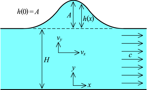
Figure 1: An illustration describing the stationary flow of a solitary wave in a co-moving frame.

2 Basic equations

Let us consider a solitary wave propagating to the left along the $-x$ direction with velocity $c$ in an unbounded fluid of ambient height $H$. Examining it from a co-moving system, the stationary flow described in Figure 1 is observed. The origin of the coordinate system is placed to the bottom of the fluid under the peak of the solitary wave. The horizontal ($v_{x}$) and vertical ($v_{y}$) components of the flow velocity are functions of the coordinates $x$ and $y$, while $h(x)$ denotes the excess fluid height compared to $H$. The amplitude of the solitary wave is defined as the value $A=h(0)$. In the limiting case of $x\rightarrow\pm\infty$, it is obvious that $v_{x}(x,y)\rightarrow c$, $v_{y}(x,y)\rightarrow 0$ and $h(x)\rightarrow 0$.

For many liquids, in particular water, the effect of viscosity can be neglected, therefore the problem can be described by the Euler equation. Instead of trying to solve it directly, we first recite some important properties of the flow to be examined: first, water is practically incompressible, hence

$$\nabla\underline{v}=0.$$ (1)

As a consequence, the density $\rho$ of the liquid is constant. It can be assumed by most wave phenomena that the flow is irrotational so that

$$\nabla\times\underline{v}=0.$$ (2)

According to the standard boundary conditions, the vertical velocity must vanish at the bottom of the liquid:

$$v_{y}=0\quad\textrm{for}\quad y=0.$$ (3)

It is also clear that the material flux through the full depth must be the same for all vertical cross-sections taken at any $x$. The constant value of this flux can be obtained by calculating it for the limiting case of $x\rightarrow\pm\infty$ such that

$$\int_{y=0}^{H+h(x)}v_{x}(x,y)dy=cH.$$ (4)

The last important property of the flow is that the liquid pressure equals the pressure of air on the surface:

$$p=p_{0}\quad\textrm{for}\quad y=H+h(x).$$ (5)

Finding a flow that satisfies conditions (1)$-$(5) is much easier than solving the Euler equation directly.

3 An iteration scheme

In this section, we present a method for obtaining an ordinary differential equation for $h(x)$ in an iterative sequence of steps. Let us first examine the flow with the velocity components

$$v_{x}(x,y)=\frac{cH}{H+h(x)}\quad\textrm{and}\quad v_{y}(x,y)=0.$$ (6)

It is clear that the conditions (2)$-$(4) are fulfilled; however, the divergence of the velocity does not vanish. To satisfy condition (1), we add a new term to the vertical velocity $v_{y}$. The new term $\Delta v_{y}$ can be obtained by elementary methods: differentiation of $v_{x}$ with respect to the coordinate $x$ and integration with respect to the single variable $y$. An arbitrary function of $x$ appears after the integration which can be chosen to fulfil condition (3). The new term obviously does not contribute to the flux, therefore the flow with these modified components satisfies conditions (1), (3) and (4).

For the new flow, however, the rotation of the velocity does not disappear; to satisfy condition (2), we now add a new term $\Delta v_{x}$ to the horizontal velocity $v_{x}$. The method for obtaining $\Delta v_{x}$ is nearly the same as above; after the differentiation of $v_{y}$ with respect to $x$ and the integration with respect to $y$ an arbitrary function of $x$ appears. This can be chosen to make the flux resulting from the new term vanish. The vertical velocity at the bottom of the water obviously remains zero, hence the flow with the new term satisfies the conditions (2)$-$(4).

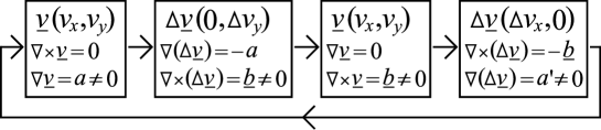
Figure 2: A flow diagram summarizing one iteration cycle, as described in the text.

At this point, the situation is formally the same as at the beginning: the divergence of the flow is non-zero again. It can be assumed, however, that after these steps we are closer to the exact flow solution. Once again, a new term must be added to the vertical velocity and another one to the horizontal velocity as mentioned above. By following this iteration scheme and repeating the steps shown in Figure 2, we obtain infinitely long expressions for both components of the velocity. Assuming that this method is convergent, the new terms become less and less significant. The remaining divergence and rotation after all the steps therefore approach zero and the limiting flow satisfies conditions (1)$-$(4).

It is, however, still left to examine whether condition (5) is fulfilled. Since viscosity can be neglected and the flow is irrotational, Bernoulli’s law holds between two points of the water surface; one of these points can be chosen to be infinitely far away, while the other is arbitrary with its horizontal coordinate $x$:

$$p_{0}+\rho gH+\frac{1}{2}\rho c^{2}=p_{0}+\rho g\big{(}H+h(x)\big{)}+\frac{1}{2}\rho\Big{[}v_{x}^{2}\big{(}x,H+h(x)\big{)}+v_{y}^{2}\big{(}x,H+h(x)\big{)}\Big{]}.$$ (7)

After rearranging this equation, both the air pressure $p_{0}$ and the density $\rho$ of water cancel out, hence we obtain

$$1-\frac{2gh(x)}{c^{2}}=\frac{v_{x}^{2}(x,H+h(x))}{c^{2}}+\frac{v_{y}^{2}(x,H+h(x))}{c^{2}}.$$ (8)

This equation determines the shape $h(x)$ of the surface. The velocity components are given by the infinitely long expressions obtained from the iteration scheme of Figure 2. Equation (8) is thus an infinitely long ordinary differential equation, which is impossible to treat without approximations.

4 Order of magnitude estimates

By substituting in principle the infinitely long expressions of $v_{x}(x,H+h(x))$ and $v_{y}(x,H+h(x))$ into equation (8) we obtain an equation containing an infinite number of complicated terms. These terms can, however, be expanded into series with respect to dimensionless quantities much less than unity. Assuming a long solitary wave of small amplitude, these quantities are

$$\frac{h(x)}{H}\ll 1\quad\textrm{and}\quad Hh^{\prime\prime}(x)\ll 1,$$ (9)

for example. The derivatives of $h(x)$ with respect to $x$ are denoted by primes. After the expansion the equation is still infinitely long, but its terms are simpler and can more easily be classified. Equation (8) can formally be written as

$$\frac{2gh(x)}{c^{2}}-\frac{2h(x)}{H}+\sum_{n=1}^{\infty}T_{n}=0,$$ (10)

where all terms denoted by $T_{n}$ take the similar form: they are the products of the function $h(x)$ and its different derivatives multiplied or divided by the appropriate power of $H$ to keep them dimensionless. Some of the terms are nonlinear, while those containing derivatives are responsible for dispersion. Examples of such terms are

$$\frac{h(x)^{2}}{H^{2}}\quad\textrm{and}\quad H\cdot h^{\prime\prime}(x).$$ (11)

Both nonlinearity and dispersion can occur in more complex terms, such as

$$H^{2}\cdot h^{\prime}(x)\cdot h^{\prime\prime\prime}(x).$$ (12)

To estimate the magnitudes of these different terms, let us write the shape of the solitary wave as

$$h(x)=A\cdot f(kx)\quad\textrm{where}\quad f(0)=1.$$ (13)

The new quantity $k$ is an ’effective wave number’, which is inversely proportional to the horizontal extension of the solitary wave, while $f$ denotes an appropriately smooth unknown function of the dimensionless product $kx$. The magnitude of the derivatives of $h(x)$ can be estimated via equation (13). For example, the magnitudes of the terms in (11) are

$$\frac{h(x)^{2}}{H^{2}}\sim\frac{A^{2}}{H^{2}}\quad\textrm{and}\quad H\cdot h^{\prime\prime}(x)\sim H\cdot Ak^{2},$$ (14)

respectively. It is assumed that the amplitude $A$ is much smaller, while the length $\sim 1/k$ is much larger than the initial water height $H$:

$$\frac{A}{H}\ll 1\quad\textrm{and}\quad kH\ll 1,$$ (15)

which are equivalent to the relations in (9).

Solitary waves emerge as a balance between nonlinearity and dispersion; in the most simplistic case, it is enough to keep the largest nonlinear and the largest dispersive term. These are the terms in (11), therefore in this case they must have the same order of magnitude: $A^{2}/H^{2}\sim HAk^{2}$, i.e.

$$\frac{A}{H}\sim k^{2}H^{2}.$$ (16)

This relation determines the relative magnitudes of the small quantities in (15). In the following section, we derive the simplest approximation, which corresponds to a case where all terms $T_{n}$ in equation (10) are neglected except for the terms in (11). The solution can be checked to be in agreement with relation (16). It is natural to expect that the same relation also holds for the more accurate approximations since keeping smaller terms does not essentially change the order of magnitude relationships.

5 First- and second-order equations

In order to derive the approximate equations, let us return to equation (6) and implement the method described in the previous two sections. First of all, we divide the velocity components by $c$, and expand the component $v_{x}$ into a Taylor series. If we keep terms up to the order of $A^{3}/H^{3}$, we obtain

$$\frac{v_{x}}{c}=1-\frac{h(x)}{H}+\frac{h(x)^{2}}{H^{2}}-\frac{h(x)^{3}}{H^{3}}\quad\textrm{and}\quad\frac{v_{y}}{c}=0.$$ (17)

Now we add a new term $\Delta v_{y}$ to the vertical velocity and hence satisfy condition (1):

$$\frac{\partial v_{x}}{\partial x}+\frac{\partial(\Delta v_{y})}{\partial y}=0.$$ (18)

By keeping terms up to the order of $A^{3}/H^{3}$, we obtain

$$\frac{\Delta v_{y}}{c}=-\frac{1}{c}\int\frac{\partial v_{x}}{\partial x}dy=\frac{h^{\prime}(x)}{H}\bigg{(}1-\frac{2h(x)}{H}\bigg{)}y+g(x).$$ (19)

The arbitrary function $g(x)$ should be chosen to be zero in order to fulfil condition (3). Next, we add a new term $\Delta v_{x}$ to the horizontal velocity to cancel out the rotation of the flow component (19):

$$\frac{\partial(\Delta v_{y})}{\partial x}-\frac{\partial(\Delta v_{x})}{\partial y}=0.$$ (20)

After the integration with respect to $y$ there remains an arbitrary function $q$ of $x$:

$$\frac{\Delta v_{x}}{c}=\frac{1}{c}\int\frac{\partial(\Delta v_{y})}{\partial x}dy=\frac{1}{2H^{2}}\Big{[}\big{(}H-2h(x)\big{)}h^{\prime\prime}(x)-2h^{\prime}(x)^{2}\Big{]}y^{2}+q(x).$$ (21)

The function $q(x)$ should be chosen to make the flux resulting from the component (21) equal to zero:

$$\int_{y=0}^{H+h(x)}\frac{1}{2H^{2}}\Big{[}\big{(}H-2h(x)\big{)}h^{\prime\prime}(x)-2h^{\prime}(x)^{2}\Big{]}y^{2}dy+q(x)\big{(}H+h(x)\big{)}=0.$$ (22)

Hence the velocity components after the first iteration cycle are given by

$$\frac{v_{x}}{c}=\bigg{(}1-\frac{h(x)}{H}+\frac{h(x)^{2}}{H^{2}}-\frac{h(x)^{3}}{H^{3}}\bigg{)}$$

$$+\frac{1}{2H^{2}}\Big{[}\big{(}H-2h(x)\big{)}h^{\prime\prime}(x)-2h^{\prime}(x)^{2}\Big{]}\bigg{(}y^{2}-\frac{1}{3}\big{(}H+h(x)\big{)}^{2}\bigg{)}$$ (23)

and

$$\frac{v_{y}}{c}=\frac{h^{\prime}(x)}{H}\bigg{(}1-\frac{2h(x)}{H}\bigg{)}y.$$ (24)

The substitution of these components into equation (8) yields

$$1-\frac{2gh(x)}{c^{2}}=\bigg{[}\bigg{(}1-\frac{h(x)}{H}+\frac{h(x)^{2}}{H^{2}}-\frac{h(x)^{3}}{H^{3}}\bigg{)}$$

$$+\frac{1}{3}\bigg{(}1+\frac{h(x)}{H}\bigg{)}^{2}\Big{[}\big{(}H-2h(x)\big{)}h^{\prime\prime}(x)-2h^{\prime}(x)^{2}\Big{]}\bigg{]}^{2}+h^{\prime}(x)^{2}$$ (25)

if we keep terms up to the order of $A^{3}/H^{3}$. The magnitude of the different terms can be estimated via equations (13) and (16), similarly as for the terms in (14):

$$\frac{h(x)}{H}\sim\frac{A}{H},\quad\frac{h(x)^{2}}{H^{2}}\sim H\cdot h^{\prime\prime}(x)\sim\frac{A^{2}}{H^{2}}$$ (26)

and

$$\frac{h(x)^{3}}{H^{3}}\sim h(x)\cdot h^{\prime\prime}(x)\sim h^{\prime}(x)^{2}\sim\frac{A^{3}}{H^{3}}.$$ (27)

Rearranging the right-hand side of equation (25) and keeping the terms up to the order of $A^{3}/H^{3}$ leads to the form (10):

$$\frac{2gh(x)}{c^{2}}-\frac{2h(x)}{H}+T_{1}+T_{2}=0,$$ (28)

where

$$T_{1}=\frac{3h(x)^{2}}{H^{2}}+\frac{2}{3}H\cdot h^{\prime\prime}(x)$$ (29)

and

$$T_{2}=-\frac{4h(x)^{3}}{H^{3}}-\frac{2}{3}h(x)\cdot h^{\prime\prime}(x)-\frac{1}{3}h^{\prime}(x)^{2}$$ (30)

are on the order of $A^{2}/H^{2}$ and $A^{3}/H^{3}$, respectively.

The simplest approximation is to neglect both $T_{1}$ and $T_{2}$ in equation (28). In this case, we obtain the linear equation

$$\bigg{(}\frac{2g}{c^{2}}-\frac{2}{H}\bigg{)}h(x)=0,$$ (31)

which describes the shallow-water linear waves of arbitrary shape. These non-dispersive waves propagate with the well-known velocity of

$$c=c_{0}=\sqrt{gH},$$ (32)

which converts equation (31) into an identity for any $h(x)$.

Nonlinear and dispersive terms are, however, both necessary for a solitary wave solution. The simplest approximation describing such solutions can be obtained by keeping $T_{1}\sim A^{2}/H^{2}$ and still neglecting $T_{2}\sim A^{3}/H^{3}$ in equation (28):

$$\frac{2gh(x)}{c^{2}}-\frac{2h(x)}{H}+\frac{3h(x)^{2}}{H^{2}}+\frac{2}{3}H\cdot h^{\prime\prime}(x)=0.$$ (33)

The first-order approximate equation (33) is, to the given approximation, equivalent to the KdV equation, which is generally used to describe solitary waves [2]. Since relation (32) is a zeroth-order solution for the propagation velocity $c$, it is worth introducing the small dimensionless quantity

$$\epsilon=1-\frac{gH}{c^{2}}\ll 1$$ (34)

and approximating the first two terms in equation (33) as

$$\bigg{(}\frac{2gH}{c^{2}}-2\bigg{)}\frac{h(x)}{H}=\bigg{[}4-4\bigg{(}1+\frac{\epsilon}{2}\bigg{)}\bigg{]}\frac{h(x)}{H}\approx\bigg{[}4-\frac{4}{\sqrt{1-\epsilon}}\bigg{]}\frac{h(x)}{H}=\bigg{(}4-\frac{4c}{\sqrt{gH}}\bigg{)}\frac{h(x)}{H}.$$ (35)

The approximation $(1+\epsilon)^{\alpha}\approx 1+\alpha\epsilon$ appears in the second step, which is valid to first order in $\epsilon$. After differentiation and multiplication by $H/4$ we obtain

$$h^{\prime}(x)-\frac{c}{\sqrt{gH}}h^{\prime}(x)+\frac{3}{2H}h(x)\cdot h^{\prime}(x)+\frac{1}{6}H^{2}h^{\prime\prime\prime}(x)=0$$ (36)

from equation (33). This ordinary differential equation is then transformed into a partial one with the independent variables $x$ and $t$. Derivatives in all terms of equation (36) must be substituted with a partial derivative either with respect to $x$ or with respect to $t$. In the latter case, however, the term also must be divided by $c$ so that equation (36) can be restored by seeking the solution in the special form $h(x+ct)$. Since the propagation velocity $c$ is different for every special wave solution, it must not explicitly appear in an equation describing such a wide range of phenomena. Only the second term in equation (36) should therefore contain a time derivative. By leaving spatial derivatives in all other terms we obtain

$$\frac{\partial h}{\partial x}-\frac{1}{\sqrt{gH}}\cdot\frac{\partial h}{\partial t}+\frac{3}{2H}h\cdot\frac{\partial h}{\partial x}+\frac{1}{6}H^{2}\frac{\partial^{3}h}{\partial x^{3}}=0,$$ (37)

the KdV equation describing waves propagating to the left.

It can be verified that further steps after the first iteration cycle do not result in new terms with magnitudes up to the order of $A^{2}/H^{2}$. For the second-order approximation, however, we must collect all terms with magnitudes up to $A^{3}/H^{3}$; this requires one more iteration cycle. If we keep terms up to the order of $A^{3}/H^{3}$, the new term $\Delta v_{y}^{\prime}$ added to the vertical velocity is given by

$$\frac{\Delta v_{y}^{\prime}}{c}=-\frac{1}{c}\int\frac{\partial(\Delta v_{x})}{\partial x}dy=-\frac{1}{6H}h^{\prime\prime\prime}(x)\Big{[}y^{3}-y\big{(}H+h(x)\big{)}^{2}\Big{]}+g(x).$$ (38)

The arbitrary function $g(x)$ is once again chosen to be zero so that the flow fulfils condition (3). By still keeping terms up to $A^{3}/H^{3}$, the new term $\Delta v_{x}^{\prime}$ added to the horizontal velocity reads as

$$\frac{\Delta v_{x}^{\prime}}{c}=\frac{1}{c}\int\frac{\partial(\Delta v_{y}^{\prime})}{\partial x}dy=-\frac{1}{24H}h^{(4)}(x)\Big{[}y^{4}-2y^{2}\big{(}H+h(x)\big{)}^{2}\Big{]}+r(x),$$ (39)

where the function $r(x)$ is chosen to make the flux resulting from the flow component (39) vanish:

$$\int_{y=0}^{H+h(x)}-\frac{1}{24H}h^{(4)}(x)\Big{[}y^{4}-2y^{2}\big{(}H+h(x)\big{)}^{2}\Big{]}dy+r(x)\big{(}H+h(x)\big{)}=0.$$ (40)

Hence the new term $\Delta v_{x}^{\prime}$ is given by

$$\frac{\Delta v_{x}^{\prime}}{c}=-\frac{h^{(4)}(x)}{360H}\Big{[}15y^{4}-30y^{2}\big{(}H+h(x)\big{)}^{2}+7\big{(}H+h(x)\big{)}^{4}\Big{]}.$$ (41)

Similarly as after the first iteration cycle, the velocity components of the net flow obtained from expressions (23), (24), (38) and (41) are substituted into equation (8), which is then rearranged to the form (10). By keeping terms up to the order of $A^{3}/H^{3}$, the three terms of $T_{2}$ in equation (30) appear with respect to equation (33). One new term, $2H^{3}h^{(4)}(x)/45$, also results from the component (41) of the second iteration cycle. The second-order approximate equation thus takes the form

$$\frac{2gh(x)}{c^{2}}-\frac{2h(x)}{H}+\frac{3h(x)^{2}}{H^{2}}+\frac{2}{3}H\cdot h^{\prime\prime}(x)-\frac{4h(x)^{3}}{H^{3}}-\frac{2}{3}h(x)\cdot h^{\prime\prime}(x)-\frac{1}{3}h^{\prime}(x)^{2}+\frac{2}{45}H^{3}h^{(4)}(x)=0.$$ (42)

By continuing the same method it is possible to obtain more accurate (higher order) approximations without too much difficulty. The calculations, however, become far more complicated, hence these further equations are beyond the scope of this paper.

6 Solitary wave solutions

In this section, we first recover the well-known properties of the KdV solitary waves from equation (33), then find a solitary wave solution for the second-order approximate equation (42). By using abbreviation (34), equation (33) reads as

$$-2\epsilon\frac{h(x)}{H}+3\frac{h(x)^{2}}{H^{2}}+\frac{2}{3}H\cdot h^{\prime\prime}(x)=0.$$ (43)

After a multiplication by $h^{\prime}(x)$ it can be integrated to give

$$-\epsilon\frac{h(x)^{2}}{H}+\frac{h(x)^{3}}{H^{2}}+\frac{1}{3}H\cdot h^{\prime}(x)^{2}=B.$$ (44)

In solitary waves $h^{\prime}(x)\rightarrow 0$ for $h(x)\rightarrow 0$, hence the integration constant $B$ is zero. By expressing $h^{\prime}(x)$ from equation (44) we obtain the separable differential equation

$$h^{\prime}(x)=\pm\sqrt{\frac{3}{H^{3}}}\cdot h(x)\sqrt{\epsilon H-h(x)}.$$ (45)

The solution for equation (45) can be obtained by elementary methods:

$$h(x)=\epsilon H\cdot\cosh^{-2}\big{(}k(x-C)\big{)},$$ (46)

where $k$ is the ’effective wave number’ given by

$$k=\sqrt{\frac{3\epsilon}{4H^{2}}}.$$ (47)

The integration constant $C$ is only responsible for shifting the wave along the $x$-axis, therefore it can be chosen to be zero without any restriction. By comparing equations (13), (46) and (47) we obtain

$$\epsilon=\frac{A}{H}=\frac{4}{3}k^{2}H^{2}$$ (48)

between the amplitude and the length of the solitary wave, clearly verifying the validity of relation (16). The propagation velocity $c$ can be expressed from equations (34) and (48) by means of the following approximation:

$$c=\frac{\sqrt{gH}}{\sqrt{1-\epsilon}}=\frac{\sqrt{gH}}{\sqrt{1-A/H}}\approx\sqrt{gH}\bigg{(}1+\frac{A}{2H}\bigg{)}.$$ (49)

Relations (48) and (49) are well known from the KdV theory of solitary waves [2], as well as the shape (46) of the wave, as plotted in Figure 3.

Figure 3: Shape of the solitary wave of the first-order equation (33) with water height $H$ = 1 and amplitude $A$ = 0.1.

Unlike the previous one, the second-order approximate equation (42) can not be solved in such an elementary way. We first examine the function $h(x)$ asymptotically, i.e. in the region where $h(x)\rightarrow 0$. By neglecting nonlinear terms in equation (42) we obtain

$$-2\epsilon\frac{h(x)}{H}+\frac{2}{3}H\cdot h^{\prime\prime}(x)+\frac{2}{45}H^{3}h^{(4)}(x)=0,$$ (50)

with abbreviation (34) used once again. Seeking the solution in the exponential form $\exp(kx)$ gives four distinct roots:

$$k_{1,2}=\pm\frac{1}{H}\sqrt{\frac{15}{2}}\cdot\Bigg{(}-1+\sqrt{1+\frac{4}{5}\epsilon}\Bigg{)}^{1/2}$$ (51)

and

$$k_{3,4}=\pm\frac{i}{H}\sqrt{\frac{15}{2}}\cdot\Bigg{(}1+\sqrt{1+\frac{4}{5}\epsilon}\Bigg{)}^{1/2}.$$ (52)

The magnitude of these roots is estimated for $\epsilon\ll 1$ to be

$$k_{1,2}\approx\pm\frac{1}{H}\sqrt{3\epsilon}\quad\textrm{and}\quad k_{3,4}\approx\pm\frac{i}{H}\sqrt{15}.$$ (53)

While the first two roots are appropriately small, the last two describe sinusoidal waves with wavelength comparable to the ambient water height $H$. Accepting such waves would contradict the second relation of (15), which is an assumption leading to equation (42). The solitary wave solution therefore must approach the real exponential functions corresponding to $k_{1,2}$ as $h(x)\rightarrow 0$: an increasing one ($k_{1}>0$) for $x\rightarrow-\infty$ and a decreasing one ($k_{2}<0$) for $x\rightarrow+\infty$.

Figure 4: Definition of the quantities $h(x_{0})$ and $A$, and the numerical solution of equation (42) with $x_{0}$ = $-$6.78, $h(x_{0})$ = 0.01 and $\epsilon$ = 0.1.

In the region between the two limiting cases, we solve equation (42) numerically. The initial values for the function $h(x)$ and its derivatives can be set according to the asymptotic form described above. If we start from a small value $h(x_{0})$ located at a large negative $x_{0}$, the derivatives have initial values

$$h^{(n)}(x_{0})=h(x_{0})\cdot k_{1}^{n}.$$ (54)

If the initial derivatives are not set according to this, short sinusoidal waves appear, leading to the above-mentioned contradiction. As long as $h(x_{0})$ is sufficiently small, changing its value only leads to a shift along the $x$-axis. For every $\epsilon$ therefore we can find a solitary wave solution with a unique shape and amplitude. The latter is read off as the maximum value of the numerically obtained function $h(x)$, as shown in Figure 4. The results obtained for different $\epsilon$ values are summarized in Table 1, along with two simple functional forms of $A/H$, the second of which appears to be a really good approximation of $\epsilon$.

• $\epsilon$	$A/H$	$A/H-A^{2}/H^{2}$	$A/H-21A^{2}/20H^{2}$
  0.01	0.0101072	0.010005	0.0099999
  0.02	0.0204382	0.020020	0.0199996
  0.03	0.0310081	0.030047	0.0299985
  0.04	0.0418337	0.040084	0.0399961
  0.05	0.0529342	0.050132	0.0499921

Table 1: The quantity $\epsilon$ versus different functional forms of $A/H$ obtained from numerical solutions of equation (42).

The relationship between $\epsilon$ and the amplitude $A$ indicates that a correction should be added to relation (48) in the case of second-order solitary waves:

$$\epsilon=\frac{A}{H}-\frac{21A^{2}}{20H^{2}}.$$ (55)

Although Table 1 only shows values of $\epsilon$ much smaller than unity, relation (55) remains approximately valid for larger values. After the critical value of $\epsilon\approx 0.25$, however, there are no solitary wave solutions; the function $h(x)$ diverges exponentially. The highest possible solitary waves are found to have the ratio $A/H\approx 0.5$. While equation (33) formally allows solitary waves of arbitrary height, equation (42) contains a hint on the experimentally observed instability (wave breaking) of high solitary waves.

Figure 5: Solitary wave of the second-order equation (42) obtained numerically with $H$ = 1 and $A$ = 0.2 (a); the same wave plotted together with the analytically known first-order wave marked by dashed line (b).

The propagation velocity can once again be expressed from equations (34) and (55). This time, however, we have to keep terms up to the order of $A^{2}/H^{2}$ to obtain the velocity for the solitary waves of the second-order equation (42):

$$c=\frac{\sqrt{gH}}{\sqrt{1-\epsilon}}=\frac{\sqrt{gH}}{\sqrt{1-A/H+21A^{2}/20H^{2}}}\approx\sqrt{gH}\bigg{(}1+\frac{A}{2H}-\frac{3A^{2}}{20H^{2}}\bigg{)}.$$ (56)

This result is equivalent to that obtained by Laitone with a systematic expansion of the flow components [4]. Note that the velocity given by expression (56) is smaller than the velocity in (49); the maximum correction, belonging to $A/H\approx 0.5$, is about $(3/80)/(5/4)\approx 3\%$. The new terms in equation (42) with respect to equation (33) are only small corrections, thus the new solitary waves plotted in Figure 5(a) are similar to those of the KdV theory. Comparison in Figure 5(b) indicates that the second-order solitary waves are slightly longer.

To summarize, the results obtained via the numerical methods show that the solitary waves of the second-order equation (42) are slower and longer than the corresponding KdV waves.

7 Velocity measurements

In order to experimentally examine the validity of the theory, we measured the propagation velocity of large amplitude solitary waves and compared the results with relations (49) and (56). Solitary waves propagating in a long, narrow glass tank were observed with a CCD camera standing in the direction perpendicular to the propagation. The experiments were carried out with coloured tap water to make the contrast between the fluid and the background larger. The rightmost part of the tank shown in Figure 6 was separated by a lock-gate and contained water of height $H^{\prime}$, larger than the height $H$ of the ambient fluid. After pulling out the lock-gate, this difference of water height generated a solitary wave propagating to the left. Solitary waves of different amplitude were produced by changing the modified water height $H^{\prime}$. The camera was placed to look at a region 6 m away from the right end of the tank to avoid transient phenomena. Reflected waves propagating to the right were also recorded.

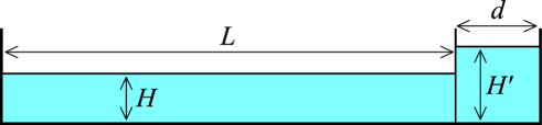
Figure 6: The initial set-up used to produce solitary waves ($L$ = 10 m, $d$ = 13 cm, $H$ = 10.3 cm, while $H^{\prime}$ varied between 17 cm and 24 cm).

The pictures taken by the camera were afterwards digitally evaluated by a computer program, which calculated the displacement of the solitary wave between subsequent images. The profile of the wave could easily be obtained by finding the border separating the dark and light regions of the picture. Intersections of the surface and different horizontal lines were used to monitor the solitary wave on subsequent images, as shown in Figure 7.

The exact value of the water height $H$ and the amplitude $A$ could also be read off by the computer program. Both values are obtained as the difference of appropriate vertical coordinates: the former is the distance between the bottom of the tank and the surface far in front of the solitary wave, while the latter is the maximum value of the surface with respect to $H$. In the case of direct solitary waves, both values $H$ and $A$ are known with the accuracy of $\pm$1.5 mm. When examining reflected waves, the maximum value used to calculate the amplitude $A$ has a larger deviation on subsequent images, hence the error of $A$ increases to $\pm$2.5 mm.

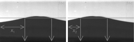
Figure 7: Two photographs taken in rapid succession ($\Delta t$ = 0.0635 s) with arrows indicating the methodology for determining the velocity of the wave: the displacement $\Delta x$ = $x_{1}-x_{2}$ = 7.54 cm gives $c$ = 119 cm s^-1.

Since the time interval between two pictures is known with a negligible relative error of $\sim$ 0.1%, the velocity can easily be obtained from the displacement. We used several subsequent images to fit a line on the relative displacements to reduce the error in the velocity. This error was estimated as the standard deviation of the different velocities obtained from tracing the left and right intersections of 9-26 horizontal lines, their number depending on the amplitude of the solitary wave. The average values of these velocities for the same wave are plotted non-dimensionally in Figure 8, with the vertical error of the points coming from two main sources. Besides the deviation in the velocity, the error in the water height $H$ must also be taken into account when calculating the Froude number

$$\mathrm{Fr}=\frac{c}{\sqrt{gH}}.$$ (57)

The theoretical predictions (49) and (56) are also plotted for comparison. Figure 8 clearly shows the coincidence of the measured points and relation (56), and indicates therefore the validity of the underlying second-order theory.

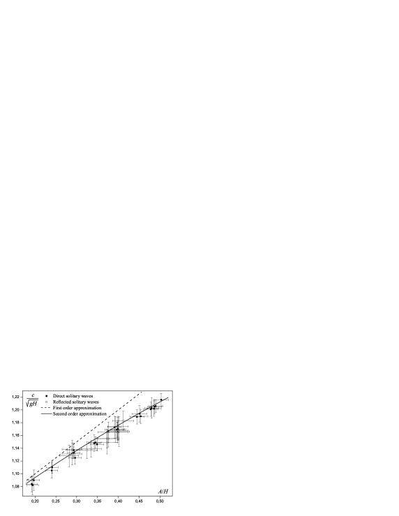
Figure 8: Dimensionless propagation velocity of the solitary waves as a function of $A/H$; the continuous lines mark the theoretical predictions (49) and (56).

8 Conclusions

The iteration scheme presented in Section 3 can be used to obtain equations describing solitary waves in arbitrary order of approximation. These equations are ordinary differential equations, therefore they only give solutions of stationary shape (one-soliton solutions). By implementing the elementary iteration scheme of Section 3, we obtained the first- and second-order approximate equations.

The first-order equation was solved in Section 6 to recover the well-known solitary waves of the KdV theory. By finding the solitary wave solutions of the second-order equation and comparing them to those of the KdV theory, we found that the second-order solitary waves are slightly slower and longer than the corresponding KdV waves. The expression obtained for their propagation velocity is equivalent to the result derived by Laitone [4]. Velocity measurements of real solitary waves show a really good correlation between the experimental results and the second-order theory, which is therefore experimentally verified to be valid.

It is worth mentioning that further refinements to the theory do not give observable corrections to the propagation velocity. By taking the third-order approximation we would obtain $c/\sqrt{gH}=1+A/2H-3A^{2}/20H^{2}+3A^{3}/56H^{3}$ [4]. In the case of the highest solitary waves with $A/H\approx 0.5$, the last term is only responsible for a maximum correction of $\approx 0.5\%$, which is very difficult to demonstrate in an experimentally reliable way. The second-order approximation is sufficient to describe shallow-water solitary waves in all realistic situations.

References

References

- [1] Drazin P G and Johnson R S 1989 Solitons: An Introduction (Cambridge University Press)
- [2] Korteweg D J and de Vries G 1895 Phil. Mag. (Ser. 5) 39 422
- [3] Friedrichs K O 1948 Commun. Pure Appl. Math. 1 81
- [4] Laitone E V 1960 J. Fluid Mech. 9 430
- [5] Fenton J 1972 J. Fluid Mech. 53 257
- [6] Schwartz L W 1974 J. Fluid Mech. 62 553
- [7] Landau L D and Lifshitz E M 1987 Fluid Dynamics (Oxford: Pergamon)
- [8] Kundu P K, Cohen I M and Hu H H 2004 Fluid Mechanics (New York: Academic)
- [9] Ludu A 2007 Nonlinear Waves and Solitons on Contours and Closed Surfaces (Berlin: Springer)