Exact nonlinear Bloch-state solutions for Bose-Einstein condensates in a periodic array of quantum wells

Abstract

A set of exact closed-form Bloch-state solutions to the stationary Gross-Pitaevskii equation are obtained for a Bose-Einstein condensate in a one-dimensional periodic array of quantum wells, i.e. a square-well periodic potential. We use these exact solutions to comprehensively study the Bloch band, the compressibility, effective mass and the speed of sound as functions of both the potential depth and interatomic interaction. According to our study, a periodic array of quantum wells is more analytically tractable than the sinusoidal potential and allows an easier experimental realization than the Krönig-Penney potential, therefore providing a useful theoretical model for understanding Bose-Einstein condensates in a periodic potential.

1 Introduction

Bose-Einstein condensates (BECs) in periodic potentials have attracted great interest both experimentally and theoretically during the past few years [1, 2]. A major reason is that they usually exhibit phenomena typical of solid state physics, such as the formation of energy bands [3, 4], Bloch oscillations [5, 6], Landau-Zener tunneling [7, 8, 9, 10] between Bloch bands and Josephson effects [11, 12], etc. The advantage of BECs in periodic potentials over a solid-state system is that the potential geometry and interatomic interactions are highly controllable. Such a BEC system can therefore serve as a quantum simulator [13] to test fundamental concepts. For instance, the Bose-Hubbard model is almost perfectly realized in the BEC field, hence enabling an experimental study of the quantum phase transition between a superfluid and Mott insulator [14, 15].

Research so far has been primarily focused on BECs in two types of periodic potentials. The first type is the sinusoidal optical lattice [1, 2]. Experimentally created by two counter-propagating laser beams, the sinusoidal optical lattice consists of only one single Fourier component. Most studies on BECs in this type of potential ask for the help of numerical simulations since analytical solutions are lacking. By contrast, the second one is the so-called Krönig-Penney potential [17, 18, 19]. In the BEC field, the Krönig-Penney potential as shown in Refs. [17, 18, 19] is usually referred to as a periodic delta function potential. However, in the original work [20] and the field of condensed matter physics [21], the Krönig-Penney potential is also used as the periodic rectangular potential. To avoid the confusion, we adopt the notion in the BEC field and refer to the Krönig-Penny potential as a periodic delta function potential. With this understanding, the periodic rectangular potential in this paper is called as a periodic array of quantum wells. The Krönig-Penny potential admits an exact solution in closed analytical form, leading to general expressions that can simultaneously describe all parameter regimes. Nevertheless, it’s very difficult to realize a Krönig-Penney potential in experiments. It is therefore instructive to seek a periodic potential that not only permits an exact solution in closed analytical form, but also is hopeful to be realized experimentally. The search for such type of potential is justified by the fact that the fundamental properties of a BEC in a periodic potential should not depend on the potential shape [18]. So theorists are actually at liberty to select the form of a periodic potential for the convenience of their study.

One such option is provided by a periodic array of quantum wells separated by barriers [21]. On the experimental side, this potential can be generated by interference of several laser beams. Since two interference counter-propagating laser beams form a sinusoidal potential that contains one single Fourier component, we expect more Fourier components to be involved by using several counter-propagating laser beams. When frequencies of these beams are multiples of the fundamental, interference of them would result in a periodic array of quantum wells. An experimental scheme to create such unconventional optical lattices has recently been demonstrated in Ref. [22]. On the theoretical side, it will be shown in this paper that exact closed-form solutions exist for a periodic array of quantum wells. In fact, such potential virtually becomes a Krönig-Penney potential, i.e., a lattice of delta functions, in the limit when the width of barriers becomes much smaller than the lattice period. We are therefore motivated to launch a systematic study on a BEC in a periodic array of quantum wells.

In this article, we derive a set of exact Bloch-state solutions to the stationary Gross-Pitaevskii equation (GPE) for a BEC in a one-dimensional periodic array of quantum wells. All our exact solutions, in the limit of varnishing interatomic interaction, are reduced to their counterparts in the linear case, i.e. the Bloch states of the stationary Schrödinger equation with a one-dimensional periodic array of quantum wells. We apply these solutions to analyze the structure of Bloch bands, the compressibility, effective mass and the speed of sound as functions of both potential depth and the strength of interatomic interaction. Special emphasis is given to the behavior of the compressibility and effective mass.

The outline of the paper is as follows. In Sec. 2, we introduce notations and describe basic theoretical framework of our study. In Sec. 3, the general solutions of GPE in a single quantum well are derived in detail. In Sec. 4, we investigate the lowest Bloch band for a BEC in a periodic array of quantum wells. A comprehensive analysis is presented in Sec. 5 that explains the dependence of Bloch band, the compressibility, effective mass and the speed of sound on the potential depth and the strength of interatomic interaction. Finally, we discuss their experimental implications followed by a summary in Sec. 6.

2 Mean-field theory of Bose-Einstein condensates

We consider a BEC is tightly confined along the radial directions and subjected to a periodic potential in x-direction. The periodic potential $V_{pot}\left(x\right)$ is assumed to be a periodic array of quantum wells in the form

$$V_{pot}(x)=\sum_{n=-\infty}^{+\infty}V_{q}(x-nT),$$ (1)

with

$$V_{q}\left(x\right)=\left\{\begin{array}[]{lcl}0&&0<x\leq a,\\ sE_{R}&&a<x\leq a+b,\end{array}\right.$$ (2)

where $a$ is the well width and $b$ is the barrier width. In Eq. (1), the $V_{pot}\left(x\right)$ has a periodicity of $T=a+b$. The $s$ in Eq. (2) is a dimensionless parameter that denotes the strength of the $V_{pot}\left(x\right)$ in units of the recoil energy $E_{R}=\hbar^{2}q_{B}^{2}/2m$, with $q_{B}=\pi/T$ being the Bragg momentum.

We restrict ourselves to the case where the BEC system can be well described by the mean-field theory. The parameter characterizing the role of interactions in the system is $g_{3D}n$, where $g_{3D}=4\pi\hbar^{2}a_{s}/m$ is the two-body coupling constant and $n$ is the 3D average density. Here $a_{s}>0$ is the 3D s-wave scattering length. At the mean-field level, descriptions of a BEC system are given by the stationary GPE (or nonlinear Schrödinger equation). In our case, the confinement along the radial direction is so tight that the dynamics of the atoms in the radial direction is essentially frozen to the ground state of the corresponding magnetic trap. As shown in Ref. [23], the effective coupling constant can be deduced as $g=g_{3D}/2l_{0}^{2}$ with $l_{0}$ being the length scale of the magnetic trap. In this limit, the stationary 3D GPE therefore reduces to a 1D equation that reads [24]:

$$\left(-\frac{\hbar^{2}}{2m}\frac{\partial^{2}}{\partial x^{2}}+V_{pot}\left(x\right)+gnT|\psi|^{2}\right)\psi\left(x\right)=\mu\psi\left(x\right),$$ (3)

where $m$ is the atomic mass, $\mu$ is the chemical potential and the order parameter $\psi(x)$ is normalized according to $\int_{0}^{T}dx|\psi(x)|^{2}=1$.

Despite non-linearity, Eq. (3) permits solutions in the form of Bloch waves [3, 25]

$$\psi_{k}(x)=e^{ikx}\phi_{k}(x),$$ (4)

where $k$ is the Bloch wave vector and $\phi_{k}(x)$ is a periodic function with the same periodicity as the $V_{pot}\left(x\right)$. We point out that Eq. (4) does not exhaust all possible stationary solutions of GP Eq. (3) due to the presence of the nonlinear term. Except for the Bloch-form solutions, the GP Eq. (3) with a periodic potential also allows other kinds of solutions, for example, period-doubled state solutions [16].

The GP equation (3), in terms of the function $\phi_{k}(x)$, can be rewritten as:

$$\left[\frac{\left(-i\hbar\partial_{x}+k\right)^{2}}{2m}+V_{pot}+gnT|\phi_{k}|^{2}\right]\phi_{k}=\mu(k)\phi_{k}.$$ (5)

Note that the chemical potential $\mu(k)$, which is derived from Eq. (5) as

$$\mu(k)=\int_{0}^{T}dx\phi_{k}^{*}\left[\frac{(-i\hbar\partial_{x}+k)^{2}}{2m}+V_{pot}+gnT|\phi_{k}|^{2}\right]\phi_{k},$$ (6)

usually does not coincide with the energy $\varepsilon(k)$ of the BEC system defined by

$$\varepsilon(k)=\int_{0}^{T}dx\phi_{k}^{*}\left[\frac{(-i\hbar\partial_{x}+k)^{2}}{2m}+V_{pot}+\frac{1}{2}gnT|\phi_{k}|^{2}\right]\phi_{k}.$$ (7)

Comparison of Eqs. (6) and (7) indicates that $\varepsilon(k)$ equals $\mu(k)$ only when interactions are absent. Generally, $\varepsilon(k)$ and $\mu(k)$ are related to each other through following definition [24, 25]

$$\mu(k)=\frac{\partial\left[n\varepsilon(k)\right]}{\partial n}.$$ (8)

Now we seek exact solutions of Eq. (3) by assuming following ansatz [17, 18, 19] for the wave function $\psi(x)$

$$\psi\left(x\right)=\sqrt{\rho\left(x\right)}\exp\left[-i\Theta\left(x\right)\right],$$ (9)

where the density function $\rho\left(x\right)$ is nonnegative and the phase function $\Theta\left(x\right)$ is real. Substituting Eq. (9) into Eq. (3) and re-scaling equations, we obtain

$$\left(\frac{\partial\rho}{\partial x}\right)^{2}=2\eta\rho^{3}+4\left(\mu-V_{pot}\right)\rho^{2}-\beta\rho-4\alpha^{2},$$ (10)

and

$$\Theta=\int dx\frac{\alpha}{\rho\left(x\right)},$$ (11)

where the length scale is $T/\pi$, the $\eta=gnT/E_{R}$ represents the nonlinear interaction, and $\beta$ and $\alpha$ are integral constants.

3 General solution in a single quantum well

We then proceed to solve the GP Eq. (10) in a single quantum well $V_{sig}$ defined by

$$V_{sig}\left(x\right)=\left\{\begin{array}[]{lcl}0&&0<x\leq a,\\ s&&a<x\leq a+b.\end{array}\right.$$ (12)

As is well known, general solutions for Eq. (10) with a constant potential can be expressed in terms of the Jacobi Elliptic functions [26, 27, 28]. In our case, we derive exact solutions to Eq. (10) separately in the two regions shown in Eq. (12).

In the region $0<x\leq a$, the $V_{sig}(x)$ is zero. Hence the exact solutions of Eq. (10) have the following general form

$$\rho_{1}\left(x\right)=A-\left[A-\frac{2\alpha^{2}}{A\left(2K^{2}+A\eta\right)}\right]SN^{2}\left(Kx+\delta,n_{1}^{2}\right),$$ (13)

where

$$n_{1}^{2} = -\frac{A}{2K^{2}}\eta+\frac{\alpha^{2}}{AK^{2}\left(2K^{2}+A\eta\right)}\eta,$$

$$\beta = -\frac{2\left(2AK^{2}+A^{2}\eta\right)^{2}+8\left(A\eta+K^{2}\right)\alpha^{2}}{2AK^{2}+A^{2}\eta},$$ (14)

$$\mu = K^{2}+\left(A+\frac{\alpha^{2}}{A\left(2K^{2}+A\eta\right)}\right)\eta.$$

In Eq. (13), $SN$ is the Jacobi elliptic sine function and $n_{1}^{2}$ denotes the modulus whose range is restricted within $[0,1]$. In this general solution, the free variables are the translational scaling $K$, the translational offset $\delta$, and the density offset $A$. In the limit of $\eta=0$, the solution (13) can be reduced to

$$\rho_{1}\left(x\right)=A-\left(A-\frac{\alpha^{2}}{AK^{2}}\right)\sin^{2}\left(Kx+\delta\right),$$ (15)

with $n_{1}=0$, $\beta=-\frac{8A^{2}K^{2}+8\alpha^{2}}{2A}$ and $\mu=K^{2}$.

In the region $a<x\leq a+b$, the $V_{sig}(x)$ is a constant. In this region, Eq. (10) admits two kinds of exact solutions, depending on whether there is a node within the barrier.

The first type of solutions contains no node within the barrier and has the form:

$$\rho_{2}\left(x\right)=B+\left[B+\frac{2\alpha^{2}}{B\left(2Q^{2}-B\eta\right)}\right]SC^{2}\left(Qx+\gamma,n_{2}^{2}\right),$$ (16)

with

$$n_{2}^{2} = 1-\left(\frac{B}{2Q^{2}}+\frac{\alpha^{2}}{BQ^{2}\left(2Q^{2}-B\eta\right)}\right)\eta,$$

$$\mu = s-Q^{2}+\left(B-\frac{\alpha^{2}}{B\left(2Q^{2}-B\eta\right)}\right)\eta,$$ (17)

$$\beta = 4BQ^{2}-2B^{2}\eta+\frac{\left(8B\eta-8Q^{2}\right)\alpha^{2}}{2BQ^{2}-B^{2}\eta}.$$

In the limit of $\eta=0$, this solution is reduced to

$$\rho_{2}\left(x\right)=B+\left(B+\frac{\alpha^{2}}{BQ^{2}}\right)\sinh^{2}\left(Qx+\gamma\right),$$ (18)

with $n_{2}=1$, $\mu=s-Q^{2}$ and $\beta=(4B^{2}Q^{2}-4\alpha^{2})/B$.

The second type of solutions admits only one node within the barrier and is expressed as

$$\rho_{2}=-\frac{B}{8Q^{2}}+\left[\frac{Q^{2}}{\eta}+\frac{B}{8Q^{2}}-\frac{Q\sqrt{BQ^{2}-16\alpha^{2}\eta}}{\sqrt{B}\eta}\right]NC^{2}\left(Qx+\gamma,n_{2}^{2}\right),$$ (19)

with

$$n_{2}^{2} = \frac{1}{2}-\frac{B}{16Q^{4}}\eta+\frac{\sqrt{BQ^{2}-16\alpha^{2}\eta}}{2\sqrt{B}Q},$$

$$\mu = s-\frac{B}{16Q^{4}}\eta-\frac{Q\sqrt{BQ^{2}-16\alpha^{2}\eta}}{\sqrt{B}},$$ (20)

$$\beta = \frac{32Q^{2}\alpha^{2}}{B}-\frac{\sqrt{B}\sqrt{BQ^{2}-16\alpha^{2}\eta}}{2Q}.$$

which again can be reduced in the limit of $\eta=0$ to:

$$\rho_{2}\left(x\right)=-\frac{B}{8Q^{2}}+\frac{B}{8Q^{2}}\cosh^{2}\left(Qx+\gamma\right),$$ (21)

with $n_{2}=1$, $\mu=s-Q^{2}$ and $\beta=(B^{2}-64Q^{2}\alpha^{2})/2B$. In Eqs. (16) and(19), $SC$ and $NC$ are also the Jacobi elliptic functions with modulus $n_{2}^{2}$ and the free variables are $B$, $Q$ and $\gamma$.

Note that all above solutions, in the limit of $\eta=0$, are nothing but the stationary solutions for the linear Schrödinger equation.

4 Bloch bands and group velocity

So far we have ignored Bloch wave condition (4) and solved the GP equation for a single quantum well for specific regions. Next we seek the global solution to the GP equation defined on the whole x axis that satisfies the Bloch wave condition.

Assume that the solutions given in Eqs. (13), (16) and (19) respectively comprise a segment of the complete Bloch wave stationary solution of the GP equation with the potential given by Eq. (1). We then extend the wave function $\psi_{k}(x)$ originally defined on $\left(0,a+b\right]$ to the whole x axis and construct the ultimate Bloch wave solution according to the Bloch condition:

$$\psi_{k}(x+T)=e^{ikT}\psi_{k}(x),$$ (22)

where $k$ is the Bloch wave vector defined by

$$k=-\Theta(x)=-\alpha\int_{0}^{T}\frac{dx}{\rho(x)}.$$ (23)

Imposing the boundary condition that the $\psi_{k}(x)$ is continuous at $x=a$ and using Eq. (22), we obtain

$$\rho_{1}\left(a\right) =\rho_{2}\left(a\right),$$ (24)

$$\partial_{x}\rho_{1}\left(a\right) =\partial_{x}\rho_{2}\left(a\right),$$ (25)

$$\rho_{1}\left(0\right) =\rho_{2}\left(T\right),$$ (26)

$$\partial_{x}\rho_{1}\left(0\right) =\partial_{x}\rho_{2}\left(T\right).$$ (27)

Two additional constraints are the continuity of the chemical potential on the boundary and the normalization condition for the wave function, i.e.

$$\mu_{1}=\mu_{2},$$ (28)

and

$$\int_{0}^{T}|\psi_{k}(x)|^{2}dx=\int\nolimits_{0}^{a}\rho_{1}\left(x\right)dx+\int\nolimits_{a}^{T}\rho_{2}\left(x\right)dx=1.$$ (29)

In principle, Eqs. (23-29) provide a complete set of equations for us to determine the unknown parameters $A$, $B$, $K$, $Q$, $\delta$, $\gamma$ and $\alpha$. Once these parameters are found, we obtain the Bloch band of the periodic system. Note that in the region $a<x\leq a+b$, the first type solution $\rho_{2}(x)$ is adopted when $k\neq\pm q_{B}$ , while the second type $\rho_{2}(x)$ is used when $k=\pm q_{B}$.

Figure 1: (a) and (b) the lowest Bloch band and group velocity with $s=5$ for $gn=0,$ $0.1E_{R}$ and $0.5E_{R}$; (c) and (d) the lowest Bloch band, group velocity with $s=5$, $10$, $15$ when $gn=0.1E_{R}$. (e) in order to compare changes of the energy band, we vertically translate the Bloch band of $gn=0.1E_{R}$ and $0.5E_{R}$ to the initial position of $gn=0$.

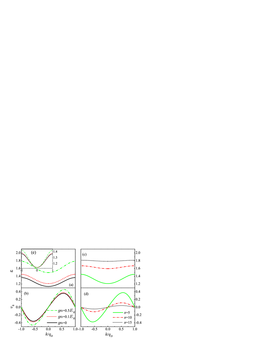
In Fig. 1, the lowest Bloch band and the corresponding group velocity as a function of quasi momentum $k$ are presented for various potential depth $s$ and interatomic interactions $gn$. Quantum well width $a=0.6$, and barrier width $b=0.4$ are used throughout this paper. Here, the group velocity is defined by $v_{k}=\partial\varepsilon/\partial k$. The states with $k=0$ and $k=\pm q_{B}$ in Fig. 1 respectively correspond to the stationary condensates at the bottom and top of the lowest Bloch band. The state with $k\neq 0$ and $k\neq\pm q_{B}$ in Fig. 1, on the other hand, describe a condensate where all atoms occupy the same single-particle wave function and move together in the periodic potential with a constant current $nv_{k}$.

Furthermore, Figs. 1 (a), (e) and (b) demonstrate that when the potential depth $s$ is fixed, the interatomic interactions affect the group velocity more conspicuously than the Bloch band. Yet for given interatomic interaction $gn$, Fig. 1 (c) and (d) show that the Bloch band becomes more and more flatter with increasing potential depth. Eventually, when the potential wells are sufficiently deep, the condensate becomes so localized in each quantum well that an adequate description can be obtained by directly using the tight-binding model [24].

5 Compressibility, Effective mass and sound speed

Now we apply our exact solutions to study the compressibility, the effective mass and the sound speed of a BEC in a periodic array of quantum wells.

We start by calculating the compressibility $\kappa$. In thermodynamics, $\kappa$ is defined as the relative volume change of a fluid or solid with respect to a pressure (or mean stress) variation. In our case, the compressibility $\kappa$ is given by[24, 25]

$$\kappa^{-1}=n\frac{\partial\mu}{\partial n}.$$ (30)

For a BEC system with repulsive interatomic interaction, the periodic potential traps atoms and enhances the repulsion. A reduced compressibility $\kappa$ is therefore expected. We illustrate this point in detail in the following.

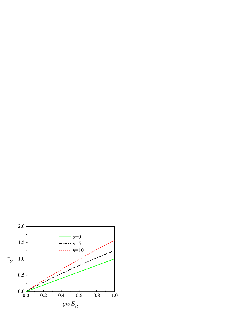
In the uniform case of $s=0$, the chemical potential is linearly dependent on the density expressed by $\mu=gn$. Thus $\kappa^{-1}=gn$ is proportional to the density. When $s\neq 0$, we substitute the general expression of $\mu$ given by Eq. (6) into Eq. ( 30), and obtain the $\kappa^{-1}$ for a BEC system in a periodic array of quantum wells. The calculated $\kappa^{-1}$ is plotted in Fig. 2 as a function of the interatomic interaction $gn$ for different $s$. The figure demonstrates that the $\kappa^{-1}$ increases with $s$, typical of a wave function localized at the bottom of each quantum wells. Compared to the uniform case, the $\kappa^{-1}$ increases linearly only for small $gn/E_{R}$. Whereas for large $gn/E_{R}$, the growth of $\kappa^{-1}$ develops a nonlinear dependence on $gn/E_{R}$.

We now give an analytical explanation to the behavior of $\kappa^{-1}$ shown in Fig. 2. Assume that $\kappa^{-1}$ is related to $s$ by the following expression [24] when $gn/E_{R}$ is small

$$\kappa^{-1}=\widetilde{g}\left(s\right)n,$$ (31)

where

$$\mu=\mu_{gn=0}+\widetilde{g}\left(s\right)n,$$ (32)

in which $\mu_{gn=0}$ depends on the potential depth, but not on density. The quantity $\widetilde{g}\left(s\right)$ in Eq. (31) acts as an effective coupling constant. In case Eq. (31) is valid, the compressibility of a BEC in a periodic array of quantum wells with $g$ is virtually transformed to the compressibility of a uniform BEC with the $\widetilde{g}(s)$. Thus by simply replacing $g$ by $\widetilde{g}(s)$, we can view our system as if there is no periodic potential [24] as far as the compressibility is concerned.

To obtain the form of $\widetilde{g}\left(s\right)$, we substitute Eq. (6) into Eq. (30) yielding [24]

$$\kappa^{-1}=n\frac{\partial\mu}{\partial n}=gn\int_{0}^{T}\phi^{4}_{\eta=0}\left(x\right)dx,$$ (33)

where $\phi_{\eta=0}$ is the ground state solution of Eq (5) for $\eta=0$. Comparison of Eq. (33) with Eq. (31) gives

$$\widetilde{g}=g\int_{0}^{T}\phi^{4}_{\eta=0}\left(x\right)dx,$$ (34)

which in our formulation has the following form:

$$\widetilde{g}=g\int_{0}^{a}\left.\rho_{1}^{2}\left(x\right)\right|_{\eta=0}dx+g\int_{a}^{T}\left.\rho_{2}^{2}\left(x\right)\right|_{\eta=0}dx,$$ (35)

where $\rho_{1}\left(x\right)$ and $\rho_{2}\left(x\right)$ are solutions respectively in well and barrier.

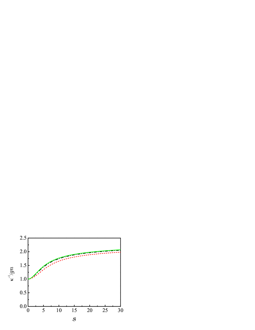
We plot the $\kappa^{-1}/gn$ as a function of the potential depth $s$ for $gn=0.1E_{R}$ and $gn=0.5E_{R}$ in Fig. 3. To compare with the behavior of the effective coupling constant $\widetilde{g}$ defined by Eq. (34), the function of $\widetilde{g}/g$ with $s$ is also plotted. Fig. 3 shows that the linear dependence of $\kappa^{-1}$ on $gn$ breaks down. However, with the increasing of $s$, the law of $\kappa^{-1}=\widetilde{g}n$ becomes to be applicable.

Figure 2: Inverse compressibility $\kappa^{-1}$ as a function of $gn/E_{R}$ for $s=0$, $5$, $10.$

Figure 3: $\kappa^{-1}/gn$ for $gn=0.1E_{R}$ (dashed-dotted line) and $gn=0.5E_{R}$ (short dashed line) as a function of the potential depth $s$, comparing with the effective coupling constant $\widetilde{g}/g$ (solid line).

We then consider the effective mass. A BEC trapped in a periodic potential can be approximately described by a uniform gas of atoms each having an effective mass $m^{\ast}$ defined by [24, 25] :

$$\frac{1}{m^{\ast}}=\left.\frac{\partial^{2}\varepsilon(k)}{\partial k^{2}}\right|_{k=0}.$$ (36)

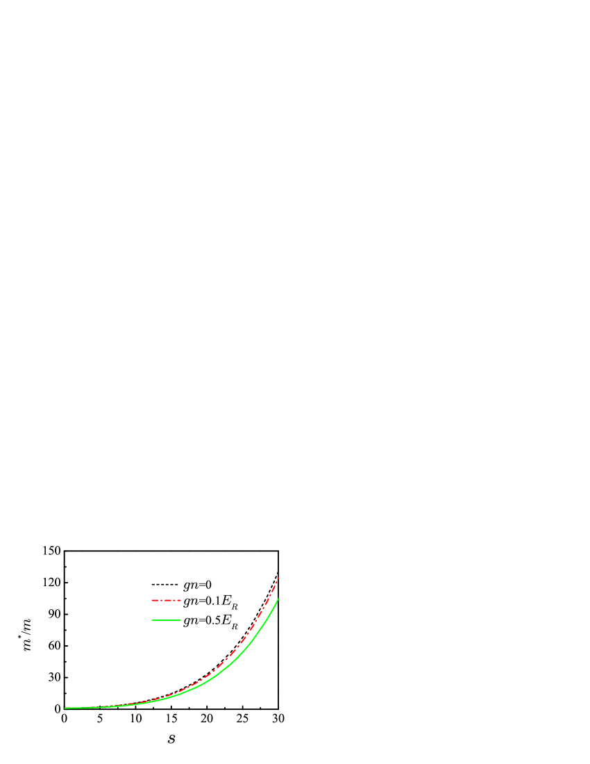
The dependence of effective mass $m^{\ast}\left(k=0\right)$ on the potential depth $s$ for $gn=0$, $gn=0.1E_{R}$ and $gn=0.5E_{R}$ is demonstrated in Fig. 4. According to Fig. 4, when $s=0$, the effective mass $m^{*}$ is reduced to the bare mass $m$. Whereas when $s$ increases, for example, to $s=30$, the $m^{*}$ becomes two orders larger in magnitude than the $m$. This increase of $m^{*}$ with $s$ can be explained by the slow-down of the particles during their tunneling through the barriers. Fig. 4 also demonstrates that the the $m^{*}$ effectively decreases with increasing interactions. This is because repulsion, contrary to the lattice potential that serves as a trap, tends to increase the width of the wave function which favors tunneling. This is the so-called screening effect of the nonlinearity [5].

As is emphasized in Ref. [24], the $m^{*}$ is determined by the tunneling properties of the system, thereby exponentially sensible to the behavior of wave function within the barriers. Thus any small change in the wave function will significantly affect the value of $m^{*}$. As a result, the conventional Gaussian approximation [24] in the tight-binding limit can not be employed to calculate the $m^{*}$. In this aspect, a periodic array of quantum wells as a solvable model, provides a better choice than the sinusoidal potential in studying the $m^{*}$ of a BEC in a periodic potential.

Figure 4: Effective mass as a function of potential depth $s$ for $gn=0$, $gn=0.1E_{R}$ and $gn=0.5E_{R}.$

Finally, we proceed to study the sound speed. Sound is a propagation of small density fluctuations inside a system [24, 25, 29, 30, 31]. The key point in studying sound is to find the sound speed. The speed of sound is important for two simple reasons: (i) it is a basic physical parameter that tells how fast the sound propagates in the system, and (ii) it is intimately related to superfluidity according to Landau’s theory of superfluid. Because of these, the sound propagation and its speed were one of the first things that have been studied by experimentalists on a BEC since its first realization in 1995 [32, 33].

The first step to derive sound speed in a BEC is to find the ground state since it acts as a media for the sound propagation. Next, one determines the sound speed by perturbing the ground state. Traditionally, there are two equivalent definitions for the sound speed [25]. In the first definition, sound is regarded as a long wavelength response of a system to the perturbations. Sound speed can be extracted from the lowest Bogoliubov excitation energy, which is characterized by the linear phonon dispersion with a finite slope. We emphasize that the physical meaning underlying the Bogoliubov spectrum is very different form that of the Bloch bands discussed in Fig. 1. The Bloch bands refer to states which involve a motion of the whole condensate through the periodic potential. However, the Bogoliubov spectrum describes small perturbations which involve only a small portion of atoms. The non-perturbed condensate acts as a medium through which the perturbed portion is moving. In other words, the Bloch band gives the energy per particle of the current states. Being multiplied by $N$, the Bloch band energies obviously exceed the energies of the Bogoliubov excitations. In the second definition, the BEC system is viewed as a hydrodynamical system. Accordingly, the sound speed in a BEC assumes following standard expression [24, 25, 30, 31]

$$v_{sound}=\frac{1}{\sqrt{\kappa m^{\ast}}}.$$ (37)

Here we adopt the second definition of sound speed in Eq. (37) in following calculations, using our previous derivation of the compressibility and effective mass.

The calculation of sound speed as a function of the potential depth $s$ is plotted in Fig. 5 for $gn=0.1E_{R}$ and $gn=0.5E_{R}$.

Figure 5: Sound speed as a function of the potential depth $s$ divided by the sound speed in the absence of lattice ($s=0$) for $gn=0.1E_{R}$ and $gn=0.5E_{R}.$

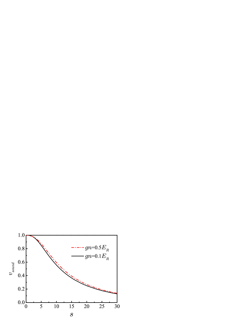
The figure demonstrates that sound velocity decreases when the potential depth is increased. This can be explained by the competition between the slowly decreasing $\kappa$ and the increasing $m^{*}$ when lattice depth is increased.

6 Conclusion

In typical experiments to date, the relevant parameters are usually chosen as follows: the interatomic interaction $gn$ ranges from $0.02E_{R}$ to $1E_{R}$ [1, 2]; the depth of the periodic potential $s$ can be adjusted from $0E_{R}$ to $12E_{R}$ [15], whereas the BEC system is still kept in the superfluid state. In particular, for a one-dimensional periodic potential, the transition to the insulator phase is expected to happen for very deep lattice. Thus there is a broad range of potential depths where the gas can be described as a fully coherent system within the framework of the mean field GPE. Hence the range of parameters in our model fit well in the current experimental conditions. Further more, a periodic array of quantum wells could be experimentally generated by the interference of serval two-counter-propagating laser beams [22]. However, we would like to point out that our study is based on GPE. In this mean-field theory, all quantum fluctuations and temperature effect are ignored. Thus in order to study the effects of temperature or fluctuations, one has to use other theories [34], especially near the transition point of superfluid and Mott insulator.

In this paper, we obtain a set of exact closed-form Bloch-state solutions to the stationary GPE for a BEC in a one-dimensional periodic array of quantum wells. These solutions are applied to calculate the Bloch band, the compressibility, effective mass and speed of sound as functions of the potential depth and the interatomic interaction. As a result, this type of periodic potential provides a useful model for further understanding of BECs.

7 Acknowledgments

We thank Biao Wu and Ying Hu for helpful discussion. R.X. and W.D.L. are supported by the NSF of China Grants No.10674087, 973 program (Nos. 2006CB921603, 2008CB317103), the NSF of Shanxi Province (Nos. 200611004), NCET (NCET-06-0259). Z.X.L. is supported by the IMR SYNL-T.S. K$\hat{e}$ Research Fellowship.

References

- [1] Morsch O and Oberthaler M 2006 Rev. Mod. Phys. 78 179
- [2] Bloch I, Dalibard J and Zwerger W 2008 Rev. Mod. Phys. 80 885
- [3] Wu Biao and Niu Qian, 2001 Phys. Rev. A 64 061603(R) Wu Biao and Niu Qian 2003 New J. Phys. 5 104
- [4] Diakonov D, Jensen L M, Pethick C J and Smith H 2002 Phys. Rev. A 66 013604 Machholm M, Pethick C J and Smith H 2003 Phys. Rev. A 67 053613
- [5] Choi Dae-Il and Niu Qian 1999 Phys. Rev. Lett. 82 2022
- [6] Morsch O, Müller J H, Cristiani M, Ciampini D and Arimondo E 2001 Phys. Rev. Lett. 87 140402
- [7] Biao Wu and Qian Niu 2000 Phys. Rev. A 61 023402
- [8] Zobay O and Garraway B M 2000 Phys. Rev. A 61 033603
- [9] Dae-Il Choi and Biao Wu 2003 Phys. Lett. A 318 558
- [10] Jona-Lasinio M, Morsch O, Cristiani M, Malossi N, Müller J H, Courtade E, Anderlini M and Arimondo E 2003 Phys. Rev. Lett. 91 230406
- [11] Anderson B P and Kasevich M A 1998 Science 282 1686
- [12] Cataliotti F S, et al. 2001 Science 293 843
- [13] Bloch I 2005 Nat. Phys. 1 23
- [14] Jaksch D, Bruder C, Cirac J I, Gardiner C W and Zoller P 1998 Phys. Rev. Lett. 81, 3108
- [15] Greiner M, Mandel O, Esslinger T, Hänsch T W and Bloch I 2002 Nature 415 39
- [16] Machholm M, Nicolin A, Pethick C J and Smith H 2004 Phys. Rev. A 69 043604
- [17] Li W D and Smerzi A 2004 Phys. Rev. E. 70 016605
- [18] Seaman B T, Carr L D and Holland M J 2005 Phys. Rev. A 71 033622 ; Seaman B T, Carr L D and Holland M J 2005 Phys. Rev. A 72 033602
- [19] Danshita I, Kurihara S and Tsuchiya S 2005 Phys. Rev. A72 053611; Danshita I and Tsuchiya S 2007 Phys. Rev. A 75 033612
- [20] Kronig R de L and Penney W G 1931 Proc. R. Soc. London 130 499
- [21] Kittel C 2005 Introduction to Solid State Physics, 8th ed. (Wiley, New York).
- [22] Ritt G, Geckeler C, Salger T, Cennini G and Weitz M 2006 Phys. Rev. A 74 063622
- [23] Olshanii M Phys. Rev. Lett. 1998 81 938.
- [24] Krämer M, Menotti C, Pitaevskii L and Stringari S 2003 Eur. Phys. J. D 27 247
- [25] Liang Z X, Dong Xi, Zhang Z D and Wu Biao 2008 Phys. Rev. A 78 023622
- [26] Bronski J C, Carr L D, Deconinck B, and Kutz J N 2001 Phys. Rev. Lett. 86 1402
- [27] Bronski J C, Carr L D, Deconinck B, Kutz J N and Promislow K 2001 Phys. Rev. E 63 036612
- [28] Li Wei Dong 2006 Phys. Rev. A 74 063612
- [29] Zaremba E 1998 Phys. Rev. A 57 518; Kavoulakis G M and Pethick C J 1998 Phys. Rev. A 58 1563; Stringari S Phys. Rev. A 58 2385 (1998); Fedichev P O and Shlyapnikov G V 2001 Phys. Rev. A 63 045601; Taylor E and Zaremba E 2003 Phys. Rev. A 68 053611
- [30] Menotti C, Krämer M, Smerzi A, Pitaevskii L and Stringari S 2004 Phys. Rev. A 70 023609
- [31] Boers D, Weiss C and Holthaus M 2004 Europhys. Lett. 67 887
- [32] Andrews M R, Kurn D M, Miesner H J, Durfee D S, Townsend C G, Inouye S and Ketterle W 1997 Phys. Rev. Lett. 79 553; Andrews M R, Stamper-Kurn D M, Miesner H J, Durfee D S, Townsend C G, Inouye S and Ketterle W 1998 Phys. Rev. Lett. 80 2967(E)
- [33] Raman C, Kohl M, Onofrio R, Durfee D S, Kuklewicz C E, Hadzibabic Z and Ketterle W 1999 Phys. Rev. Lett. 83 2502
- [34] Petrov D S, Shlyapnikov G V and Walraven J T M 2001 Phys. Rev. Lett. 87 050404