A Panoply of Cepheid Light Curve Templates

Abstract

We have generated accurate $V$ and $I$ template light curves using a combination of Fourier decomposition and principal component analysis for a large sample of Cepheid light curves. Unlike previous studies, we include short period Cepheids and stars pulsating in the first overtone mode in our analysis. Extensive Monte Carlo simulations show that our templates can be used to precisely measure Cepheid magnitudes and periods, even in cases where there are few observational epochs. These templates are ideal for characterizing serendipitously discovered Cepheids and can be used in conjunction with surveys such as Pan-Starrs and LSST where the observational sampling may not be optimized for Cepheids.

1. Introduction

The Cepheid Period-Luminosity (PL) relation is a fundamental rung in the astronomical distance ladder. With the Hubble Space Telescope (HST) routinely resolving stellar populations in nearby galaxies, Cepheid distances can potentially be calculated for a large number of new systems. In this paper, we show that high quality template light curves can accurately fit pulsation periods and mean luminosities to sparsely sampled Cepheid observations. It is our hope that these templates can be used to characterize Cepheids in archival as well as new observations, even when the time sampling of observations has not been optimized for Cepheid studies.

Principal component analysis (PCA) has found application in a wide range of astronomical studies (e.g., Faber, 1973; Conselice, 2006). The motivation behind PCA is that it can greatly reduce the number of variables required to describe a data set. By performing an eigenvalue decomposition, PCA can be used to generate a small number of eigenvectors that describe the majority of the variance in a data set. In the case of Cepheid variables, one could use PCA analysis to construct light curves with the smallest possible number of free parameters. Ideally, all Cepheids with identical periods would have a single unique light curve shape. In this case only a period, an average magnitude and a phase would be needed as free parameters to fit a light curve.

The classical technique for determining a stellar pulsation period is to calculate a “string length” (Lafler & Kinman, 1965; Burke et al., 1970). A light curve is folded along a trial period and a string length is computed by summing distances between points consecutive in phase. The trial period with the shortest computed string length is taken as the true period. This method is accurate for well sampled light curves with small photometric errors, but has been supplanted by recent techniques.

More robust periods can be obtained by fitting template light curves. Fourier analysis of Cepheids was introduced in Schaltenbrand & Tammann (1971), and Stetson (1996) generated templates based on Fourier decomposition of MW and LMC stars. Tanvir et al. (2005) used principal component analysis (PCA) to construct a large set of well sampled Cepheid observations. In this paper, we extend the techniques of Tanvir et al. (2005) to include short period Cepheids as well as first overtone Cepheids.

Short period Cepheids (with periods less than $\sim 10$ days) have been excluded from many studies for a variety of reasons. First, LMC Cepheids may show a discontinuity in the PL-relation at 10 days, casting uncertainty on their utility as reliable standard candles (Ngeow & Kanbur, 2008). Second, there is the possibility of confusion between fundamental and first-overtone mode Cepheids that have similar periods but different PL-relations. Third, if fainter stars like short period Cepheids are used to estimate distances, incompleteness bias can skew the derived distances to smaller values (Sandage & Carlson, 1988; Freedman et al., 2001). Finally, the shorter period Cepheids show more variation in light curve shape, making template construction more daunting. Keeping these potential problems in mind, we boldly go forward and derive short period templates regardless.

The outline of the paper is as follows: In Section 2, we describe generating template light curves using PCA from a large literature sample of Cepheid stars. In Section 3 we perform Monte Carlo simulations to determine how precisely we can recover Cepheid parameters using our templates. In Section 4, we discuss the process of converting fit parameters into a distance measure.

2. Principal Component Analysis

2.1. Training Set Selection

Following Tanvir et al. (2005), we perform PCA on $V$ and $I$ band light curves simultaneously. We therefore gathered light curves for stars that have both $V$ and $I$ measurements. The majority of our template stars come from the Optical Gravitational Lensing Experiment (OGLE) databases for the LMC (Udalski et al., 1999a) and SMC (Udalski et al., 1999b). We gathered additional LMC observations from Sebo et al. (2002) and additional LMC and SMC light curves from Moffett et al. (1998). Our Galactic Cepheid sample was compiled from light curves in the VizieR database (Ochsenbein et al., 2000), including data presented in Berdnikov (1997) and Berdnikov & Turner (2001). We also included Galactic Cepheids from the McMaster Cepheid Photometry and Radial Velocity Data Archive which includes light curves from many sources (Gieren, 1981; Moffett & Barnes, 1984; Coulson & Caldwell, 1985; Berdnikov & Turner, 1995; Henden, 1996; Barnes et al., 1997). We would have liked to include light curves from the MACHO survey. However the MACHO survey uses non-traditional “blue” and “red” filters that are non-trivial to convert to $V$ and $I$.

To be included in our analysis we required each light curve have at least 15 epochs of observations in both $V$ and $I$, with the exception of well spaced light curves from Berdnikov & Turner (2001), where we only demand 6 epochs in both $V$ and $I$. The initial sample contained 3173 light curves, with 248 Milky Way LCs, 1378 LMC LCs, and 1514 SMC LCs. Unlike the majority of previous Cepheid studies, we did not exclude stars with periods shorter than 10 days from the analysis. We fit Fourier components to every light curve and rejected 305 outliers (i.e., those with unusual light curve shapes or poor fits). The final sample included 150 MW Cepheids 677 LMC Cepheids, 689 SMC Cepheids, and 1171 overtone pulsators from the LMC (549 stars), SMC (575 stars), and MW (47). The period distributions of these stars are plotted in Figure 1.

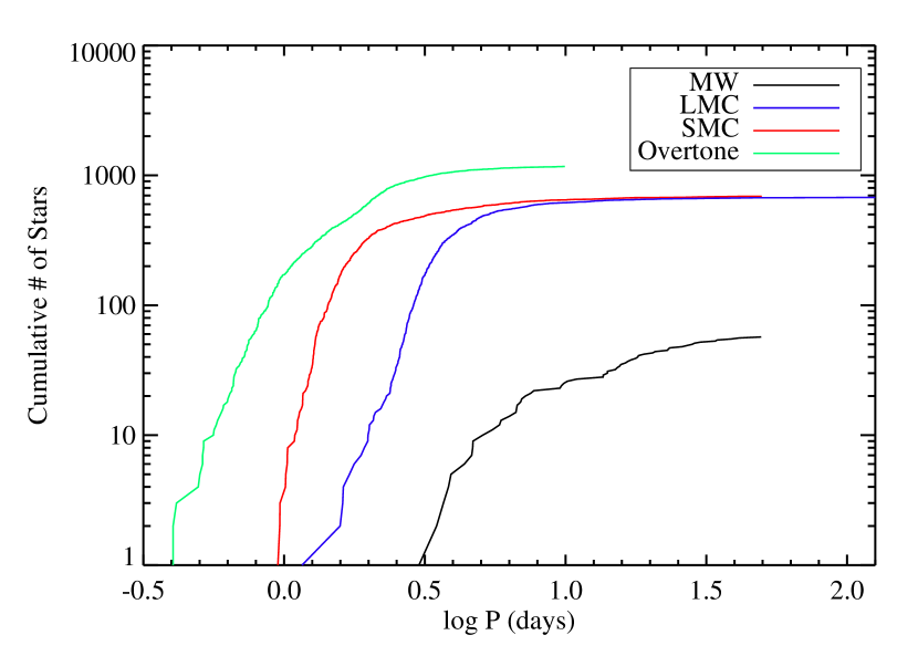
Figure 1.— Period distribution of the stars that are used to generate our templates. The Milky Way, LMC, and SMC fundamental mode stars along with the combined LMC and SMC first overtone pulsators are plotted.

The OGLE database does not distinguish between fundamental mode Cepheids and Cepheids pulsating in the first overtone mode. Figure 3 shows our simple cuts in period-magnitude space used to provisionally classify OGLE stars as fundamental or overtone pulsators. For the rest of the stars, we use the source catalog designation of overtone or fundamental Cepheid. Color-magnitude diagrams of the OGLE are plotted in Figure 2.

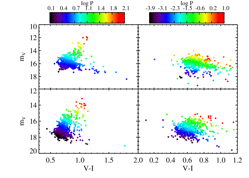
Figure 2.— Color-magnitude plots for the OGLE stars, uncorrected for reddening. Points have been color-coded by pulsation period. The upper panels show LMC stars while the lower panels show SMC stars. Fundamental mode pulsators are shown on the left and first-overtones are on the right.

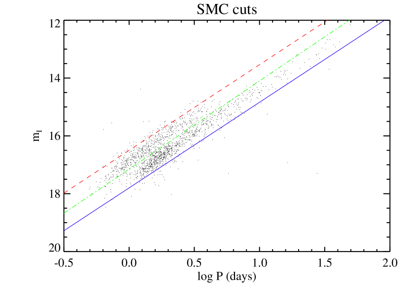
Figure 3.— First pass classification between fundamental mode and first overtone from the LMC and SMC OGLE data. Stars between the solid blue and dash-dot green line are provisionally labeled as fundamental mode and stars between the dash-dot green and dashed red are labeled as first-overtone. The lines have a slope of -3 and y-intercepts of 17.2,16.65,15.9 for the LMC and 17.8,17.15, and 16.5 for the SMC.

We initially decompose each light curve in our sample into Fourier components by fitting the following equations to the $V$ and $I$ light curves simultaneously.

$$m_{I}(t)=m_{I,0}+\sum_{k=1}^{k=8}\alpha_{k}\sin{(2\pi kt/P)}+\beta_{k}\cos{(2\pi kt/P)}$$ (1)

$$m_{V}(t)=m_{V,0}+\sum_{j=1}^{j=8}\alpha_{j}\sin{(2\pi jt/P)}+\beta_{j}\cos{(2\pi jt/P)}.$$ (2)

where $P$ is the period, $t$ is the Julian day of the observation, $m_{I,0}$ and $m_{V,0}$ are the average magnitudes in each band, and the $\alpha$ and $\beta$ terms are the Fourier amplitudes. We constrain $\beta_{j=1}$ to zero to impose a common phase for all the fits. These Fourier fits generate the 32 $\alpha$ and $\beta$ values for each star that are used in the principal component analysis. While the shapes of the light curves are fitted simultaneously, the average magnitudes in each band are completely independent. This ensures our light curve templates are not dependent on the various dust corrections (or lack thereof) that have been applied in our different source catalogs.

Ngeow et al. (2003) discuss how fitting Fourier components to sparsely sampled data can result in poor fits (see their Figure 2b for an example of how Fourier decomposition can fail for sparsely sampled light curves). To keep our fits constrained to reasonable shapes, we create a smooth light curve by linearly interpolating each observed Cepheid to include 50 points evenly distributed across the full phase of the light curve. We then fit the Fourier components of this smoothed light curve, and use the results as the initial guess for the fitting of the observed data points. In the final fit, each Fourier component is allowed to change by a maximum of 20% from the smoothed fit parameters, thereby preventing divergences compared to the smooth fit. Figure 4 shows typical results for out fitted Fourier components. Figures 5 and 6 show the distribution of the 16 best fit $\alpha$ and $\beta$ values for all of the fundamental and overtone $I$-band light curves.

Figure 4.— Example of an OGLE 2.8 day period Cepheid with the solid curves showing the best fit Fourier decomposition. The upper curve shows the $I$-band while the lower curve shows $V$. The sparse sampling in the $V$-band around a phase of 1.0 and 1.2 allows the fit slightly too much freedom (The curve rises slightly in those two regions). By performing the PCA analysis over many hundreds of light-curves, such discrepancies should be averaged out.

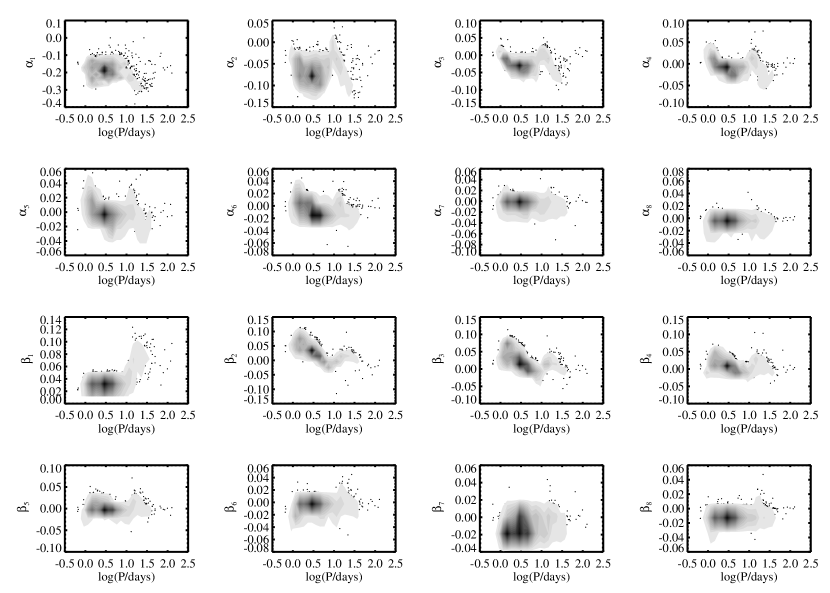
Figure 5.— The distribution of Fourier decomposition parameters for the best fits to all fundamental mode Cepheids in the $I$-band. For each population of stars, we fit low order polynomials to these Fourier component versus period plots and reject stars from further analysis that are more than 3$\sigma$ outliers. The number of stars in our sample is large enough that we have plotted contours in the densely populated regions and individual points in the sparsely sampled regions.

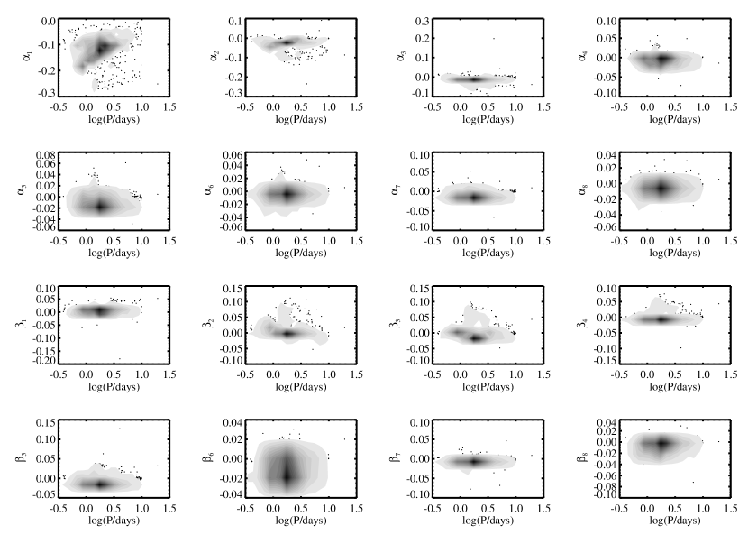
Figure 6.— Best fit Fourier components for the overtone Cepheids in the $I$-band. The distributions for the high order coefficients are concentrated near zero, implying these light curves are simply sinusoidal, an unsurprising result for stars commonly referred to as “sinusoidal” or sCepheids.

2.2. PCA Template Construction

To test for differences in Cepheid populations, we constructed templates based on various subsets of the data. In particular, we made templates that include all our fundamental mode Cepheids and subsets which included only LMC stars, only SMC stars, only short period stars, only long period stars, and only overtones. For each subsample, we first subtracted an average light curve from each measured light curve. We then performed a PCA on the residuals to develop eigenvectors that can be used to correct for deviations from the average light curve. In all cases, over 90% of the variance could be described with only four principal component eigenvectors (Table 1). An example of an average light curve and PCA eigenvectors are plotted in Figure 7.

Table 1Percentage of the total variance contained in each PCA component for each of our constructed templates.

Model	PCA1	PCA2	PCA3	PCA4	Total
	%	%	%	%	%
short period	70.1	18.7	4.8	1.4	95.1
long period	64.1	16.6	6.8	2.9	90.4
LMC	66.7	15.6	9.8	1.8	94.0
SMC	70.1	17.2	6.0	1.5	94.8
overtones	82.8	6.0	3.0	1.0	92.9

We plot the PCA vector strengths as a function of period in Figure 8. Several of the PCA vectors show strong trends with period. This is fortunate (and not too surprising), as it means while fitting for a star’s period, we can simultaneously make an educated guess as to what the corresponding shape parameters should be.

Before performing PCA, we needed 32 Fourier components, as well as two magnitudes, a period and a phase to accurately fit a Cepheid light curve. After performing PCA $>$90% of the variation in the light curve’s shape can be described with just four eigenvector amplitudes. As a final step we note that the eigenvector amplitudes are strong functions of period, allowing us to make a quality template fit with only four free parameters (two average magnitudes, a phase, and a period). Figure 8 does show one possible pitfall as the first PCA vector for the short period stars shows a great deal of scatter and little trend with period. We therefore caution that it is possible this eigenvector amplitude should be left as a free parameter if possible when fitting a light curve.

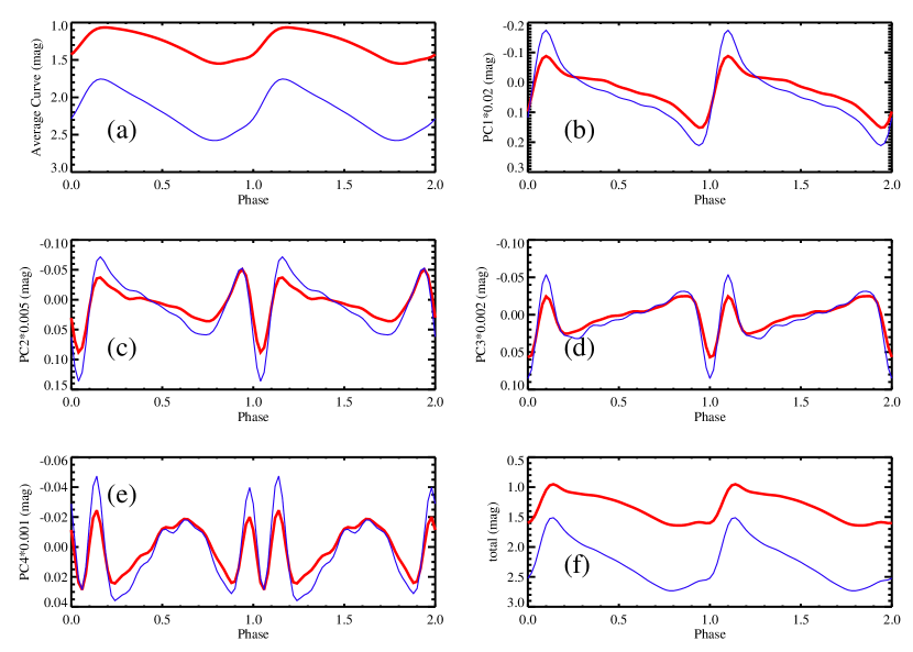
Figure 7.— The average light curve (a) and eigenvectors from the fundamental Cepheid principal component analysis. $I$-band is shown in thick red while $V$-band is shown in blue. The first PCA vector (shown in b) primarily controls the magnitude of pulsation, while the other PCA vectors (c-e) control the exact shape of the sawtooth rise of the light curve. Template light curves are constructed as linear combinations of these vectors, an example of which is shown in (f). Typical coefficients for these vectors are plotted in Figure 8.

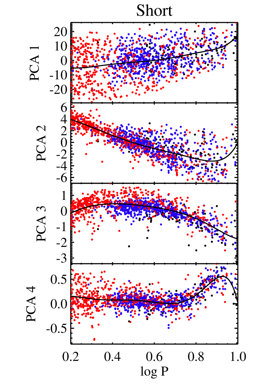
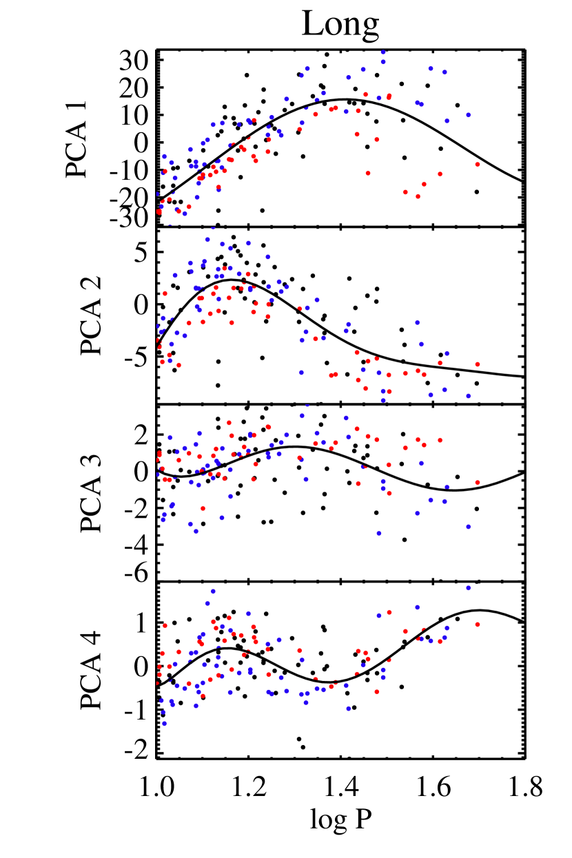
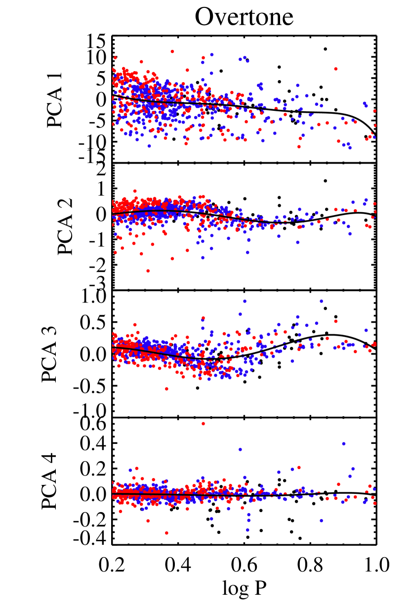
Figure 8.— The template PCA coefficients (all multiplied be a factor of $10^{3}$) for all the fundamental mode Cepheids. The SMC, LMC, and MW stars are shown by red, blue, and black points respectively. Our polynomial fits are plotted as solid curves. We have separated long period, short period, and overtone Cepheids into the left, middle, and right panels respectively.

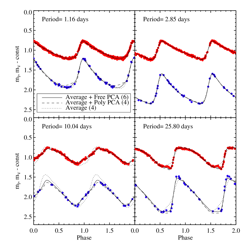
Figure 9.— Examples of four OGLE fundamental mode Cepheids fit with our derived templates. Both the $V$ and $I$ light curves are fit simultaneously. Dotted lines show the best-fitting curve if we fit with just the average light-curve (PCA eigenvectors fixed at zero), dashed curves show the best fit if we set the PCA eigenvectors to the best polynomial fit values for the given period, solid curves show the fit if we leave the first two PCA vectors as free parameters. The numbers in parentheses show the total number of free parameters in each fit.

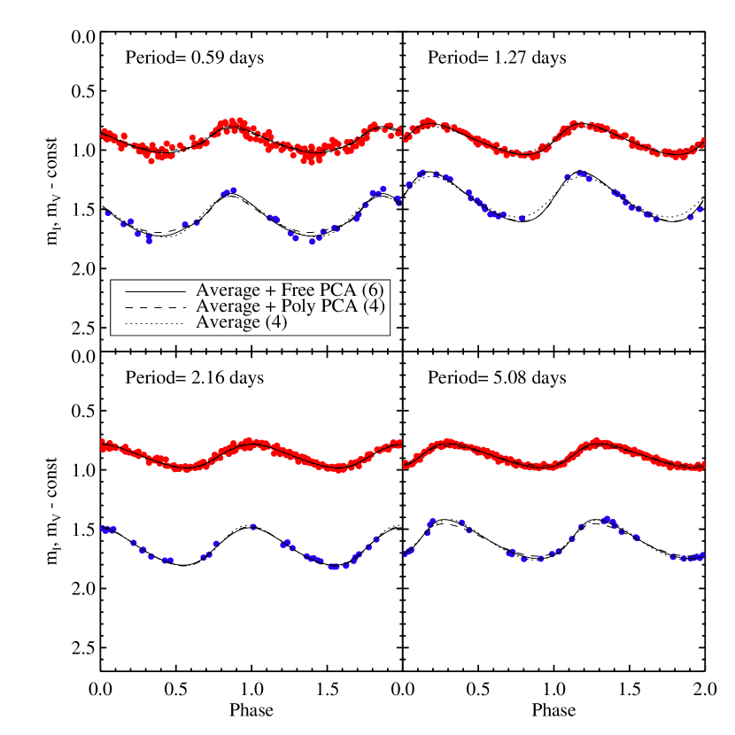
Figure 10.— Same as Figure 9, only now for Cepheids identified as first-overtones and fit with our overtone template. Again, it does not seem necessary to leave the PCA amplitudes as free parameters to converge on a quality fit.

3. Template Fitting Accuracy

Tanvir et al. (2005) have already demonstrated that the template fitting technique is superior to other common period estimation techniques for cases where the photometry is noisy. They show magnitudes and periods determined through template fitting can reduce the scatter in distance estimates by 30% compared to simple string length methods.

We now endeavor to use Monte Carlo simulations to quantify how well our templates can recover magnitudes and periods from photometry of Cepheid stars. We have developed a fitting routine that uses Levenberg-Marquardt least-squares minimization to find the best fitting Cepheid light curve, given a set of $V$ and $I$ photometry. The best fitting template is found by varying period, phase, $<I>$, and $<V>$. We have included an option to vary the amplitude of the PCA eigenvectors. Fitting sparsely sampled light curves, there is a risk of aliasing or converging on local $\chi^{2}$ minima. To avoid such problems, we use a series of initial guess periods and phases to ensure we find the global $\chi^{2}$ minimum.

Our Monte Carlo varies four parameters to judge their impact on our fitting routine’s robustness: First, we compare 5 well sampled Cepheids from the OGLE database with different periods; Second, we vary the total number of observations in each band; Next, we look at possible effects of template mis-match (fitting LMC stars with a template derived from SMC stars, fitting overtone stars with fundamental mode templates and vice-versa); Finally, we vary the photometric precision of the light curve points.

Table 2 The different epoch samplings used in our Monte Carlo error analysis.

Model	$I$ observations	$V$ observations	total
1	20	15	35
2	10	5	15
3	5	3	8
4	4	2	6

For each realization the star was randomly sampled in both bands. Therefore there are $N_{I}+N_{V}$ unique epochs of observations and we do not explicitly model observing strategies that observe in multiple filters simultaneously.

We used four fundamental mode Cepheids (periods of 2.5, 4.2, 16.0, and 20.7 days), and one overtone (period 2.5 days) from the OGLE LMC data set for the Monte Carlo tests. All the photometry has initial errors of order 0.013 mags in both bands. Although there could be some objection to using stars which are included in the PCA analysis, our sample sizes are large enough that the addition or subtraction of a few stars should make little difference to our final templates.

For the error analysis, we fit for only period, $m_{v}$, $m_{I}$, and phase. We rely on the polynomial fits in Figure 8 to give reasonable amplitudes for the PCA eigenvectors. We also folded the original light curves so that the photometry covers at most 3 periods. This restriction is needed to keep the fitting procedure from falling into local minima caused by aliasing. When fitting sparsely sampled data over a long baseline a more brute-force exploration of period parameter space would be required than our current fitting procedure.

Figure 11 shows an example of one of our fitting simulations. As expected, the errors are largest for the overtone Cepheid when fit with the wrong template. We also show the calculated uncertainties reported by our fitting routine in Figure 11. In general, the reported uncertainties are a good match to the actual errors resulting from the fits. The one exception is that the overtone uncertainties are under-estimated as a result of making the assumption that the reduced $\chi^{2}$ should be unity, which is clearly incorrect in the case of fitting an overtone with a fundamental mode template. When we use an overtone template, there is a clear improvement in the $\chi^{2}$ values, indicating that it is a better fit.

We have also explored possible template mismatches due to metallicity by repeating the Monte Carlo experiment using an SMC template ([Fe/H]$\sim-0.7$) to fit LMC stars ([Fe/H]$\sim-0.3$). The resulting periods and magnitudes are practically identical, suggesting that the templates can be used across different metallicity populations.

Figure 11.— Results of our Monte Carlo simulation where we recover Cepheid properties using our templates and least-squares fitting procedure. We fit 5 different stars, along with the 5 different observing strategies listed in Table 2. The four panels on the left show the errors in fitting magnitudes and periods and the corresponding error in distance modulus. On the right, we show the uncertainties returned by our least-squares fitting routine. With photometric errors of 0.01 mags and only 6 total epochs of observations, the uncertainties of the fitted parameters result in only a 0.1 mag uncertainty in $\Delta\mu^{0}_{fit}$.

Figure 12.— Same as Figure 11, only now the photometric errors have been increased to 0.2 mag. Again, the actual errors (left side) and very similar to the returned uncertainties (right side).

A proper assessment of the errors of individual measurements is key for determining a proper $P$-$L$ relation. We have therefore compared the uncertainties reported by our fitting procedure to the true offsets seen in our Monte Carlo re-sampling. Overall, the returned uncertainties are comparable to the actual errors derived from the Monte Carlo analysis. When the photometric errors were low (0.01 mag), the returned uncertainties were slightly too small (by $\sim$15%). On the other hand, when the errors were high and the sampling was sparse, the returned uncertainties were slightly larger than the true Monte Carlo calculated errors. Typically, around 10% of the fits would fail catastrophically, usually caused by aliasing or very sparse sampling. These failures could readily be seen as poor $\chi^{2}$ values or by visual inspection. This seems to imply that we can use the returned uncertainties, but as we will see later, observing strategy also affects the results and it is probably best to simply run a Monte Carlo for the photometric error and uncertainties for the specific sampling frequency used by a given observing program.

We ran several simulations to test how sensitive our fits are to the phase coverage of the observations. Generally, if the observations do not span more than half of the full phase, there is a large likelihood (10%-40%) that the fitted period will catastrophically fail (defined as a final fitted distance error of $>$10%).

To illustrate how well our fitting procedure works, we compared our template fits to fits using a simple asymmetric saw-tooth function. The results are plotted in Figure 13. When the light curves are well sampled, the templates and saw-tooth converge to practically identical values. In the sparsely sampled case (only 7 observational epochs), the templates return accurate fits in 4 out of 5 cases while the saw-tooth function fits fail in every case.

In summary, our tests indicate that our PCA template technique can fit periods with an precision of $\pm 0.1-0.3$ days with only 6 epochs and photometric precision of 0.01 mag. If the number of epochs increases to 15 days, our uncertainty drops to $\pm 0.03-0.2$ days.

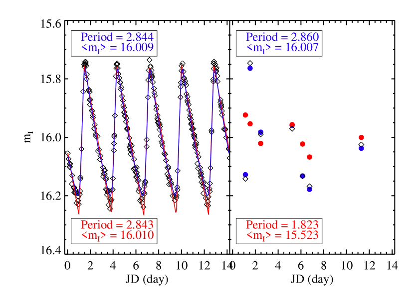
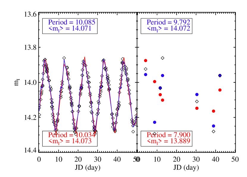
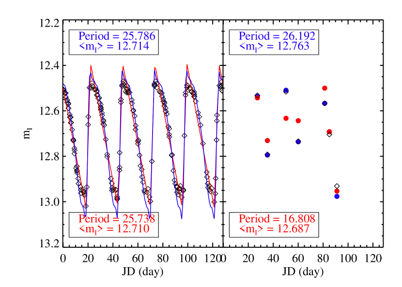
Figure 13.— An example of how effective our templates can be at fitting sparsely sampled data. In the left hand panels are the $I$-band light curves from Figure 9 fitted with our LMC templates (blue) and a simple asymmetric saw-tooth function (red). The right hand panel shows the results when 7 random points from the light curve are sampled and the the fitting is repeated. In four of the 5 cases, the templates are able to fit accurate average magnitudes and periods. The larger number of free parameters in the saw-tooth function prevents it from properly converging in the sparsely sampled cases.

4. Converting Fits to Distances

Having established that our templates can accurately fit Cepheid periods and average magnitudes, we now point out some of the potential pitfalls in using fitted parameters to derive accurate distances. In theory, distances from single Cepheids can be averaged together to find a precise distance to a galaxy. Besides the usual systematic errors associated with photometry, there are additional caveats that apply when observing a sample of Cepheids: (1) Cepheids used for a distance calculation must be above the completeness limit of the observations, otherwise, faint short-period stars will be under-sampled and the final calculated distance will be biased (Sandage & Carlson, 1988; Freedman et al., 2001); (2) If the Cepheids do not sample the full range of the instability strip, they can be offset from a standard PL-relation. Mager et al. (2008) discuss how the scatter in the PL-relation in the outskirts of NGC 4258 (Macri et al., 2006) is greatly reduced because the Cepheids populate a limited region of the instability strip; (3) Finally, there is always the risk that a Cepheid may not be de-blended from a nearby optical/physical companion. Blending is expected to bias Cepheid distance measurements to smaller values (Stanek & Udalski, 1999; Mochejska et al., 2000, 2004).

In a companion paper (McCommas et al., 2009), we have successfully applied our templates to HST data. Figure 14 shows some examples of how well the templates can fit noisy and sub-optimally sampled data. The templates only start to fail for the star with the longest period, where only half of the full phase is observed.

Figure 14.— Example of $V$ and $I$ light curves of Cepheids in M81 observed with HST and fit with our templates. See McCommas et al. (2009) for a larger sample of Cepheids and a full distance calculation to M81. The fitted period in the lower right is poorly constrained due to the sparse phase coverage.

4.1. Metallicity Effects on Light Curve Shape

There is some question as to whether the shape of the light curve can be used to determine the metallicity of a Cepheid (Paczyński & Pindor, 2000; Kanbur et al., 2002). Looking at the long period Cepheids (Figure 8), the first and second principal components have systematically smaller values for the SMC stars compared to the LMC and MW, suggesting the shapes might be intrinsically different. We use a 2D Kolmogorov-Smirnov test to compare the distributions in the PCA-Period distributions (the MW, LMC, and SMC long period variables all have very similar period distributions). The LMC and MW are consistent (Probability $>$ 0.12) with being drawn from the same populations for all of the PCA vectors (i.e., the shape of the light curve at a given period does not show significant differences). The SMC shows a significant difference between the MW (P=0.008) and LMC (P=0.04) in the distribution of the first PCA vector, but not the higher order PCA vectors. While the SMC light curve shape is different on average, there is little hope of assigning a metallicity to an individual star based on its light curve shape, since the intrinsic scatter within the SMC is larger than the differences from the LMC or MW. Even with the large number of stars in our sample, it is difficult to differentiate between the low metallicity SMC Cepheids and the higher metallicity LMC and MW Cepheids. It is possible, in theory, to observe enough long period stars that one could distinguish if a population was high or low metallicity based on the PCA distribution. However, it would require a prohibitively large sample size, as well as sufficient phase coverage that the shape parameters could be measured robustly.

Unlike the long period variables, the short period Cepheids in the three systems have very different period distributions. However, the PCA distributions overlap to a sufficiently large degree (Figure 8) that light curve shape cannot readily be used to measure the metallicity of individual stars.

While we find metallicity does not alter light curve shapes significantly, there is evidence that metallicity differences can alter the PL-relation. Several studies claim to find a metallicity dependence (Kennicutt et al., 1998; Sakai et al., 2004; Macri et al., 2006; Saha et al., 2006; Romaniello et al., 2008; Sandage & Tammann, 2008), while others find that the PL-relation is constant across galaxies (Udalski et al., 2001; Gieren et al., 2005).

5. Conclusions

We have extended the principal component analysis techniques of Tanvir et al. (2005) to generate template light curves of Cepheid variables and first-overtone variables. We have used a Monte Carlo simulation to demonstrate how robustly our templates can be used to fit Cepheid periods and magnitudes. Unlike previous studies, we do not limit ourselves to stars with periods longer than 10 days. Finally, we demonstrate the effectiveness of our templates on HST data and show that our techniques can be used to fit accurate periods and luminosities even when the observations have not been optimally spaced for observing variable stars. Our templates open up a new regime of distance measurement possibilities by enabling accurate fits for long period, short period, and overtone Cepheids from noisy and sparsely sampled observations.

References

- Barnes et al. (1997) Barnes, III, T. G., Fernley, J. A., Frueh, M. L., Navas, J. G., Moffett, T. J., & Skillen, I. 1997, PASP, 109, 645
- Berdnikov (1997) Berdnikov, L. N. 1997, VizieR Online Data Catalog, 2217, 0
- Berdnikov & Turner (1995) Berdnikov, L. N., & Turner, D. G. 1995, Pis ma Astronomicheskii Zhurnal, 21, 803
- Berdnikov & Turner (2001) —. 2001, ApJS, 137, 209
- Burke et al. (1970) Burke, Jr., E. W., Rolland, W. W., & Boy, W. R. 1970, JRASC, 64, 353
- Conselice (2006) Conselice, C. J. 2006, MNRAS, 373, 1389
- Coulson & Caldwell (1985) Coulson, I. M., & Caldwell, J. A. R. 1985, South African Astronomical Observatory Circular, 9, 5
- Faber (1973) Faber, S. M. 1973, ApJ, 179, 731
- Freedman et al. (2001) Freedman, W. L., Madore, B. F., Gibson, B. K., Ferrarese, L., Kelson, D. D., Sakai, S., Mould, J. R., Kennicutt, Jr., R. C., Ford, H. C., Graham, J. A., Huchra, J. P., Hughes, S. M. G., Illingworth, G. D., Macri, L. M., & Stetson, P. B. 2001, ApJ, 553, 47
- Gieren (1981) Gieren, W. 1981, ApJS, 47, 315
- Gieren et al. (2005) Gieren, W., Storm, J., Barnes, III, T. G., Fouqué, P., Pietrzyński, G., & Kienzle, F. 2005, ApJ, 627, 224
- Henden (1996) Henden, A. A. 1996, AJ, 111, 902
- Kanbur et al. (2002) Kanbur, S. M., Iono, D., Tanvir, N. R., & Hendry, M. A. 2002, MNRAS, 329, 126
- Kennicutt et al. (1998) Kennicutt, Jr., R. C., Stetson, P. B., Saha, A., Kelson, D., Rawson, D. M., Sakai, S., Madore, B. F., Mould, J. R., Freedman, W. L., Bresolin, F., Ferrarese, L., Ford, H., Gibson, B. K., Graham, J. A., Han, M., Harding, P., Hoessel, J. G., Huchra, J. P., Hughes, S. M. G., Illingworth, G. D., Macri, L. M., Phelps, R. L., Silbermann, N. A., Turner, A. M., & Wood, P. R. 1998, ApJ, 498, 181
- Lafler & Kinman (1965) Lafler, J., & Kinman, T. D. 1965, ApJS, 11, 216
- Macri et al. (2006) Macri, L. M., Stanek, K. Z., Bersier, D., Greenhill, L. J., & Reid, M. J. 2006, ApJ, 652, 1133
- Mager et al. (2008) Mager, V. A., Madore, B. F., & Freedman, W. L. 2008
- McCommas et al. (2009) McCommas, L., Yoachim, P., et al P. 2008, Accepted by AJ
- Mochejska et al. (2000) Mochejska, B. J., Macri, L. M., Sasselov, D. D., & Stanek, K. Z. 2000, AJ, 120, 810
- Mochejska et al. (2004) —. 2004, IAU Colloq. 193, 310, 41
- Moffett & Barnes (1984) Moffett, T. J., & Barnes, III, T. G. 1984, ApJS, 55, 389
- Moffett et al. (1998) Moffett, T. J., Gieren, W. P., Barnes, III, T. G., & Gomez, M. 1998, ApJS, 117, 135
- Ngeow & Kanbur (2008) Ngeow, C., & Kanbur, S. 2008, ArXiv e-prints, 805
- Ngeow et al. (2003) Ngeow, C.-C., Kanbur, S. M., Nikolaev, S., Tanvir, N. R., & Hendry, M. A. 2003, ApJ, 586, 959
- Ochsenbein et al. (2000) Ochsenbein, F., Bauer, P., & Marcout, J. 2000, A&AS, 143, 23
- Paczyński & Pindor (2000) Paczyński, B., & Pindor, B. 2000, ApJ, 533, L103
- Romaniello et al. (2008) Romaniello, M., Primas, F., Mottini, M., Pedicelli, S., Lemasle, B., Bono, G., François, P., Groenewegen, M. A. T., & Laney, C. D. 2008, A&A, 488, 731
- Saha et al. (2006) Saha, A., Thim, F., Tammann, G. A., Reindl, B., & Sandage, A. 2006, ApJS, 165, 108
- Sakai et al. (2004) Sakai, S., Ferrarese, L., Kennicutt, Jr., R. C., & Saha, A. 2004, ApJ, 608, 42
- Sandage & Carlson (1988) Sandage, A., & Carlson, G. 1988, AJ, 96, 1599
- Sandage & Tammann (2008) Sandage, A., & Tammann, G. A. 2008, ArXiv e-prints, 803
- Schaltenbrand & Tammann (1971) Schaltenbrand, R., & Tammann, G. A. 1971, A&AS, 4, 265
- Sebo et al. (2002) Sebo, K. M., Rawson, D., Mould, J., Madore, B. F., Putman, M. E., Graham, J. A., Freedman, W. L., Gibson, B. K., & Germany, L. M. 2002, VizieR Online Data Catalog, 214, 20071
- Stanek & Udalski (1999) Stanek, K. Z., & Udalski, A. 1999, ArXiv Astrophysics e-prints
- Stetson (1996) Stetson, P. B. 1996, PASP, 108, 851
- Tanvir et al. (2005) Tanvir, N. R., Hendry, M. A., Watkins, A., Kanbur, S. M., Berdnikov, L. N., & Ngeow, C. C. 2005, MNRAS, 363, 749
- Udalski et al. (1999a) Udalski, A., Soszynski, I., Szymanski, M., Kubiak, M., Pietrzynski, G., Wozniak, P., & Zebrun, K. 1999a, Acta Astronomica, 49, 223
- Udalski et al. (1999b) —. 1999b, Acta Astronomica, 49, 437
- Udalski et al. (2001) Udalski, A., Wyrzykowski, L., Pietrzynski, G., Szewczyk, O., Szymanski, M., Kubiak, M., Soszynski, I., & Zebrun, K. 2001, Acta Astronomica, 51, 221