A Holographic model for Non-Relativistic Superconductor

Abstract:

We build a holographic description of non-relativistic system for superconductivity in strongly interacting condensed matter via gauge/gravity duality. We focus on the phase transition and give an example to show that a simple gravitational theory can provide a non-relativistic holographical dual description of a superconductor. There is also a critical temperature like the relativistic case, below which a charged condensation field appears by a second order phase transition and the (DC) conductivity becomes infinite. We also calculated the frequency dependent conductivity.

1 Introduction and Summary

AdS/CFT correspondence is one of the most important results from string theory [1], which maps a conformal gauge field theory on the boundary to string theory in asymptotically anti de Sitter spacetimes. A semi-classic version of this duality has appeared as gauge/gravity duality and such duality has become a powerful tool to understand the strongly coupled gauge theory and it was extended to describe aspects of strongly coupled QCD such as properties of quark gluon plasma in heavy ion collisions at RHIC [2, 3, 4] and hadron physics.

More recently, it has been attempted to use this correspondence to describe certain condensed matter systems such as the Quantum Hall effect [5] , Nernst effect [6, 7, 8], superconductor  [19] [20] [21] and FQHE (fractional quantum hall effect)  [22]. All of these phenomena have dual gravitational descriptions. As pointed in  [23], there is a large class of interesting strongly correlated electron and atomic systems that can be created and studied in experiments. In some special conditions, these systems exhibit relativistic dispersion relations, so the dynamics near a critical point is well described by a relativistic conformal field theory. It is expected that such field theories which can be studied holographically have dual AdS geometries. To describe more non-relativistic condensed matter systems, this duality has even been extended to non-relativistic conformal field theory which has Schr$\ddot{\textrm{o}}$dinger symmetry  [23].

In condensed matter systems, traditional theories are based on two themes. One is Landau Fermi liquid theory and the other is symmetry breaking. High $T_{c}$ superconductor is a phenomena waiting for a new theory. Conventional superconductors are well described by BCS theory [9] while some basic aspects of unconventional superconductors, including the pairing mechanism, remain to be understood. There are many hints that the normal state in these materials can not be described by the standard Fermi liquid theory [10] and many of unconventional superconductors, such as the cuprates and organics, are layered and much of the physics is 2+1 dimensional.

In  [19], a model of a strongly coupled system which develops superconductivity was developed based on the holography, which is an Abelian-Higgs model in a warped space time. While the electrons in real materials are non-relativistic, the model in  [19] is for relativistic system. Therefore it is natural to ask whether one can develop a similar theory with non-relativistic kinematics. The purpose of this paper is to answer this question. The boundary field theory in our model is 2+1 dimensional. However, due to the structure of non-relativistic AdS/CFT correspondence [24], bulk theory of our model should be 4+1 dimensional. We use a complex scalar field to describe the charged condensation field. We analyze the Abelian-Higgs Model in the gravity background which is dual to thermal non-relativistic ( NR ) conformal field.

In the present work, we find that there is also a critical temperature like the relativistic case, below which a charged condensation field appears by a second order phase transition and the (DC) conductivity becomes infinite. In particular, we find that as the non-relativistic parameter increases, the condensation happens more observably. We also calculated the frequency dependent conductivity and find that as the non-relativistic parameter increases, the transition happens more observably and frequency positions of peaks move away from the $\omega=0$ axis.

2 Holographic Abelian Higgs model in non-relativistic regime

2.1 Gravity for NR conformal field

AdS/CFT correspondence has been extended to describe non-relativistic condensed matter system recently  [23, 24, 25]. In the present work, we start with the the gravity background with a black hole coming from Null Melvin Twist of the planar Schwarzschild anti-de Sitter black hole  [23]

$$\textrm{d}s_{\textrm{Einstein}}^{2} = r^{2}\,k^{-\frac{2}{3}}\,\biggr{[}-\beta^{2}\,r^{2}\,f\,(\textrm{d}t+\textrm{d}y)^{2}-f\,\textrm{d}t^{2}+\textrm{d}y^{2}+k\,\textrm{d}{\bf x}^{2}\biggr{]}+k^{\frac{1}{3}}\,\frac{\textrm{d}r^{2}}{r^{2}\,f}\ .$$

In light cone coordinates, the above metric turns to be

$$\textrm{d}s^{2} = r^{2}\,k^{-\frac{2}{3}}\biggr{[}\left(\frac{1-f}{4\beta^{2}}-r^{2}\,f\right)\,\textrm{d}u^{2}+\frac{\beta^{2}r_{+}^{4}}{r^{4}}\,\textrm{d}v^{2}-\left(1+f\right)\,\textrm{d}u\,\textrm{d}v\biggr{]}$$ (1)

$$\quad+\;\;k^{\frac{1}{3}}\,\left(r^{2}\textrm{d}{\bf x}^{2}+\frac{\textrm{d}r^{2}}{r^{2}\,f}\right),$$

where

$$f=1-\frac{r_{+}^{4}}{r^{4}}\ ,\qquad k=1+\beta^{2}\,r^{2}\,(1-f)=1+\frac{\beta^{2}\,r_{+}^{4}}{r^{2}}.$$ (2)

The light cone coordinates are

$$u=\beta\,(t+y)\ ,\qquad v=\frac{1}{2\,\beta}\,(t-y).$$ (3)

$\beta$ is a non-relativistic parameter and we choose $\beta=1$ in the present work if no specification. $r_{+}$ determines the Hawking temperature of the black hole  [23]

$$T=\frac{r_{+}}{\pi\,\beta}\,.$$ (4)

This black hole is 4+1 dimensional, and so will be dual to a 2+1 dimensional non relativistic theory. The metric (1) has asymtotic Schr$\ddot{\textrm{o}}$dinger symmetry, which can be easily found if we set $r_{+}=0$. By the view of gauge/gravity, this black hole can be expected to describe non-relativistic strongly correlated quantum criticality. We shall use some probe fields to uncover the transition in the following subsection.

2.2 The model

We start with the background of a black hole with asymtotic Schr$\ddot{\textrm{o}}$dinger symmetry (1)

$$\textrm{d}s^{2}=r^{2}\,k^{-\frac{2}{3}}\biggr{[}(\frac{1-f}{4\beta^{2}}-r^{2}f)\textrm{d}u^{2}+\frac{\beta^{2}r_{+}^{4}}{r^{4}}\textrm{d}v^{2}-(1+f)\textrm{d}u\textrm{d}v\biggr{]}+k^{\frac{1}{3}}(r^{2}\textrm{d}{\bf x}^{2}+\frac{\textrm{d}r^{2}}{r^{2}f})\,.$$ (5)

In this background, we now consider a Maxwell field and a charged complex scalar field. The action turns to be

$$S=\int\textrm{d}^{5}x\sqrt{-g}\biggr{[}-\frac{1}{4}F^{ab}F_{ab}-V(|\Psi|)-|\partial\Psi-iA\Psi|^{2}\,\biggr{]}.$$ (6)

For simplicity and concreteness, we choose the quadratic potential and ignore the higher terms

$$V(|\Psi|)=2\,\widetilde{a}|\Psi|^{2}\ ,$$ (7)

where $\widetilde{a}$ is a negative constant parametrizing the symmetry breaking. Due to plane symmetric ansatz, $\Psi=\Psi(r)=\psi$, equation of motion of the scalar field is

$$\begin{split}\biggr{\{}-8\widetilde{a}r^{7}f\beta^{2}k^{1/3}+r\biggr{[}4r^{4}(2-r^{2})\beta^{2}+r_{+}^{4}(1+4(r^{2}-1)\beta^{2}+4\beta^{4})\biggr{]}\phi^{2}\biggr{\}}\psi\qquad\\ +4r^{4}f\beta^{2}\left[r^{4}(4+f)\psi^{\prime}+r^{5}f\psi^{\prime\prime}\right]=0,\end{split}$$ (8)

where the scalar potential $\phi$ is the electric potential in the axial gauge $A_{i}=0$ so that $A_{u}\doteq A_{v}=\phi(r)$ . We shall rewrite the Lagrangian with $\psi$ and $\phi$, thus the equation for the scalar potential $\phi$ is

$$\begin{split}&6k^{1/3}\phi\psi^{2}\biggr{\{}r_{+}^{8}\biggr{[}4\left(r^{2}-1\right)\beta^{4}+4\beta^{6}+\beta^{2}\biggr{]}-4r^{6}\left(r^{2}-2\right)\beta^{2}\\ &+r^{2}r_{+}^{4}\biggr{[}4\left(r^{2}-1\right)\beta^{2}+\left(-4r^{4}+8r^{2}+4\right)\beta^{4}+1\biggr{]}\biggr{\}}\\ &+fr\biggr{\{}3r\biggr{[}-r_{+}^{8}\left(4\left(r^{2}-1\right)\beta^{4}+4\beta^{6}+\beta^{2}\right)+4r^{6}\left(r^{2}-2\right)\beta^{2}\\ &+r^{2}r_{+}^{4}\left(-4\left(r^{2}-1\right)\beta^{2}+4\left(r^{4}-2r^{2}-1\right)\beta^{4}-1\right)\biggr{]}\phi^{\prime\prime}\\ &+\biggr{[}r_{+}^{8}\left(-4\left(5r^{2}+1\right)\beta^{4}+4\beta^{6}+\beta^{2}\right)+12r^{6}\left(5r^{2}-6\right)\beta^{2}\\ &+r^{2}r_{+}^{4}\left(-12\left(r^{2}+1\right)\beta^{2}+4\left(17r^{4}-22r^{2}+3\right)\beta^{4}+3\right)\biggr{]}\phi^{\prime}\biggr{\}}=0,\end{split}$$ (9)

where $\psi^{2}$ is the, in our case, $r$ dependent mass. The charged condensate has triggered a Higgs mechanism in the gravity background.

3 Numerical results

3.1 Condensation

To compute the expectation value of operators in dual field theory, we need the asymptotic behaviors of equations (8) and (9). In the limit $r\rightarrow\infty$, we find the equations of motion for $\psi$ and $\phi$ become

$$\begin{split}r^{2}\psi^{\prime\prime}+5r\psi^{\prime}-(2\widetilde{a}+\phi^{2})\psi&=&0,\\ r^{2}\phi^{\prime\prime}+5r\phi^{\prime}-2\psi^{2}\phi&=&0,\end{split}$$ (10)

where we can define a new quantity $a=\widetilde{a}+\frac{1}{2}\mu^{2}$. The asymptotic solution of equation (8) is

$$\begin{split}\psi\rightarrow r^{-\lambda_{+}}C_{1}+r^{-\lambda_{-}}C_{2},\end{split}$$ (11)

with $\lambda_{\pm}=2\pm\sqrt{4+2a}$ and the asymptotic behavior of (9) is

$$\phi\rightarrow\mu-{\rho\over r^{4}}\,,$$ (12)

where $\mu$ and $\rho$ are chemical potential and charge density. By AdS/CFT correspondence, we can interpret the coefficients $C_{\pm}$ as the expectation values of the operator $O_{\pm}$ whose conformal dimension is $\lambda_{\pm}$ respectively. We will fix one of them, and compute the other.

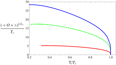
Figure 1: We plot expectation values of the operators as a function of temperature. As $\lambda_{+}=2+\sqrt{4+2a}$ increases, the condensation increases. The red real line is for $a=-1.5$, the green line is for $a=-1.2$ and the blue real line is for $a=-1$.

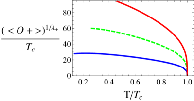
Figure 2: We focus on condensation in $a=-1$ case and show them with different non-relativistic parameter $\beta$. The blue line is for $\beta=1$, the green dashed line is for $\beta=1.5$ and the red line is for $\beta=2$.

In figure 1, we show the behavior of the expect values of condensation field as the temperature goes down. We find that below a critical temperature $T_{c}$, the condensation field appears and obtains finite value. As argued in  [21], here increasing $\lambda_{+}$ corresponds to increasing the mass of the bulk scalar. This figure shows that as the condensation field becomes heavier, the transition happens more observably. In figure 2, it shows that, as the non-relativistic parameter becomes larger, the condensation happens more observably. We can find difference between non-relativistic case and relativistic case from this figure. As shown in  [23], $\beta$ is proportional to Galilean mass in non-relativistic system, then we can see that non-relativistic particles with a heavier Galilean mass can condense more observably. We argue that a very small $\beta$ in non-relativistic can be closed to relativistic case.

We find the behavior of order parameter near the critical temperature with different $a$ and $\beta$ can be described by an universal exponent

$$<O_{+}>\;\varpropto\;T_{c}(1-T/T_{c})^{\xi}$$ (13)

where $\xi\approx 1/3$.

3.2 Conductivity

We shall compute the conductivity in the dual conformal field theory as a function of frequency. As first, we want to solve fluctuations of the vector potential $A_{x}$ in the bulk. The Maxwell equation at zero spatial momentum and with a time dependence of the form $e^{-i\omega u}$ gives

$$\begin{split}3r\left(r^{2}+r_{+}^{4}\right)\biggr{[}-r_{+}^{4}\omega^{2}+2r^{2}\left(r^{4}-r_{+}^{4}\right)\left(1+\frac{r_{+}^{4}}{r^{2}}\right)^{1/3}\psi^{2}\biggr{]}A_{x}&\\ -\left(r^{4}-r_{+}^{4}\right)\biggr{[}\left(9r^{6}+3r^{2}r_{+}^{4}+11r^{4}r_{+}^{4}+r_{+}^{8}\right)A_{x}^{\prime}&\\ +3r\left(r^{6}-r^{2}r_{+}^{4}+r^{4}r_{+}^{4}-r_{+}^{8}\right)A_{x}^{\prime\prime}\biggr{]}&=0\,.\end{split}$$ (14)

To compute the retarded (causal) green function, we solve this equation with ingoing wave boundary conditions at the horizon [18]:

$$A_{x}\propto(r^{4}-r_{+}^{4})^{-{i\omega\over 4r_{+}}}.$$ (15)

The asymptotic behavior of the Maxwell field at large radius turns to be

$$A_{x}=A_{x}^{(0)}+\frac{A_{x}^{(1)}}{r^{2}}+\cdots$$ (16)

In a rough way, the AdS/CFT dictionary tells us that the dual source and expectation value for the current are given by

$$A_{x}=A_{x}^{(0)}\,,\qquad\langle J_{x}\rangle=A_{x}^{(1)}\,.$$ (17)

Now from Ohm’s law we can obtain the conductivity

$$\sigma(\omega)=\frac{\langle J_{x}\rangle}{E_{x}}=-\frac{\langle J_{x}\rangle}{\dot{A}_{x}}=-\frac{i\langle J_{x}\rangle}{\omega A_{x}}=-\frac{iA_{x}^{(1)}}{\omega A_{x}^{(0)}}\,.$$ (18)

More concretely, we can calculate the conductivity from the correlation function. The term in the action which contains two derivatives with respect to $r$ is

$$\begin{split}S&=-{1\over 4}\int\textrm{d}r\textrm{d}^{4}x\sqrt{-g}g^{rr}g^{xx}\partial_{r}A_{x}\partial_{r}A_{x}+\cdots\\ &=\int\textrm{d}r\textrm{d}^{4}xF(r)\partial_{r}A_{x}\partial_{r}A_{x}+\cdots\end{split}$$ (19)

The retarded Green function in Minkovski space is

$$G_{R}=-F(r)A_{x}A_{x}^{\prime}\biggr{|}_{r\rightarrow+\infty}\,,$$ (20)

where

$$F(r)={fr^{3}\over 2k^{1/3}}\,.$$ (21)

The conductivity is given by

$$\sigma(\omega)={1\over i\omega}G_{R}={-F(r)A_{x}A_{x}^{\prime}\over i\omega}\biggr{|}_{r\rightarrow+\infty}.$$ (22)

From (15), we can see that

$$\sigma(\omega)={A_{(1)}\over i\omega A_{(0)}}\,,$$ (23)

which is same as the result in (18).

Figure 3: A.C conductivity for NR superconductors. Each plot is at the temperature below the critical temperature $T/T_{c}\approx 0.1$. The red line is the real part and the blue line is the imaginary part. In this figure, $a=-0.5$.

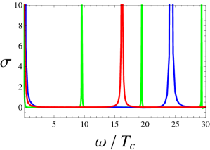
Figure 4: Conductivity for NR superconductors. In this figure, for fixed $a=-0.5$, we can see real parts of conductivities with different non-relativistic parameter $\beta$. The blue, red and green line corresponds to $\beta=1.5$, $\beta=1$, $\beta=0.5$ respectively.

In figure 3, the real part of $\sigma(\omega)$ is infinity at $\omega=0$, as shown in the figure apparently. We can also see this pole at $\omega=0$ from the imaginary part. We have multiple peaks for the conductivity. These peaks show that there are also more frequency modes which have relative large conductivities. Similar results for relativistic superconductor have been found in  [21] [20], but so far we have no direct physical interpreting for these peaks. From numerical process, these peaks comes from terms of high powers of $r$ in EOM of $A_{x}(r)$, which is the same as the case in  [20], and there similar peaks have also been interpreted as quasi-particle excitations. In our case, we can consider that $A_{x}$ is not just a perturbation but a heavy field, then its corresponding boundary vector excitations can appear. We can calculate the spectral function by $-2\textrm{Im}G$ . In our model, these peaks may be such vector quasi-particles.

Actually, when we increase $a$, we find the peaks move to $\omega=0$ axis. We also computed the difference among conductivities with different non-relativistic parameter $\beta$ in the Figure 4. We find that, as $\beta$ decreases, the frequency positions of peaks move to the $\omega=0$ axis. It seems reasonable when we consider that $\beta$ reflects the mass of non-relativistic particles, for a bigger $\beta$, the transition happens more observably and peaks are farther from the $\omega=0$ axis.

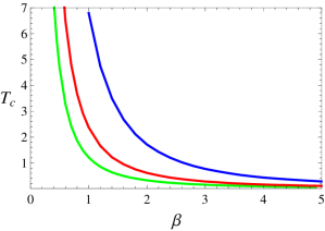
Figure 5: Critical temperature is plotted as a function of $\beta$. In this figure, the critical temperature decreases as non-relativistic parameter $\beta$ increases. The blue, red and green lines correspond to $a=-0.5$, $a=-1$ and $a=-1.5$ respectively.

In figure 5, we observe that the critical temperature will decrease as non-relativistic parameter $\beta$ increases. It implies that as the non-relativistic particle is heavier, the transition temperature turns smaller. Note that $\beta$ contributes the mass of fundamental particles, not the mass of the quasi-particles in condensed matter system.

4 Conclusion

In the present work, we built a holographic model for the strongly interacting non-relativistic system showing superconductivity. We used a black hole background which satisfies an asymptotic Schrodinger symmetry to describe the non-relativistic strongly correlated condensed matter system. We introduced a two components $A_{u}=A_{v}=\phi$ field to describe the electric field and a complex scalar to describe the condensed field. There is also a critical temperature like the relativistic case, below which a charged condensate field appears by a second order phase transition and the (DC) conductivity becomes infinite. In particular, we find that as the non-relativistic parameter increases, the condensation happens more observably. We also calculated the frequency dependent conductivity and find that as the non-relativistic parameter decreases, frequency positions of peaks move to the $\omega=0$ axis.

After we almost finished the present work, we note that the work [26] extends the holographic model to the phase which covers fermions, like the phase before superconductor transition. Two such fermions may bound a quasi-particle to interpret our peaks. This model can give interesting result like fermi-surface for the non-fermi liquid. And the work [27] gives more concrete program to describe condensed matter system holographically. All these methods can be easily used for relativistic critical phenomena. However, constructing holographic non-relativistic model for critical phenomena is still an unsolvable problem since we can not easily get a good asymptotic behavior of bulk field in the non-relativistic gravity background (after light cone transformation of the original coordinates). We introduce an extra field component in $v$ direction for electric field to solve this problem and give an example for the non-relativistic superconductor. More details about non-relativistic holographic construction for the strongly correlated system need to investigate.

Before the present letter, many works about holographic quantum critical system appeared. We hope similar methods can be used for the better construction of holographic model of the non-relativistic quantum critical phenomena in the future.

Appendix

A. calculation of conductivity

The Maxwell field $A=A_{\mu}\textrm{d}x^{\mu}$, where

$$A_{\mu}=(0,0,A_{x},0,0)\,,$$ (24)

$$x^{\mu}=(t,r,x,y,v)\,.$$ (25)

The metric $G$ is given by

$G_{5\times 5}(g_{\mu\nu})=\left(\begin{array}[]{ccccc}r^{2}k^{-2/3}({1-f\over 4\beta^{2}}-r^{2}f)&0&0&0&-{r^{2}\over 2}k^{-2/3}(1+f)\\ 0&{k^{1/3}\over r^{2}f}&0&0&0\\ 0&0&r^{2}k^{1/3}&0&0\\ 0&0&0&r^{2}k^{1/3}&0\\ -{r^{2}\over 2}k^{-2/3}(1+f)&0&0&0&r^{2}k^{-2/3}\beta^{2}{r_{0}^{4}\over r^{4}}\end{array}\right)\,,$

where

$$f=1-{r_{0}^{4}\over r^{4}},\quad k=1+\beta^{2}{r_{0}^{4}\over r^{2}}\,.$$ (26)

Then the inverse metric $G^{-1}$ is

$G_{5\times 5}^{-1}(g^{\mu\nu})=\left(\begin{array}[]{ccccc}{(1-f)k^{2/3}\over((f-1)r^{2}-1)r^{2}f}&0&0&0&{k^{2/3}(1+f)\over 2((f-1)r^{2}-1)r^{2}f}\\ 0&{r^{2}f\over k^{1/3}}&0&0&0\\ 0&0&{1\over r^{2}k^{1/3}}&0&0\\ 0&0&0&{1\over r^{2}k^{1/3}}&0\\ {k^{2/3}(1+f)\over 2((f-1)r^{2}-1)r^{2}f}&0&0&0&{(1-f-4fr^{2})k^{2/3}\over 4((f-1)r^{2}-1)r^{2}f}\end{array}\right)\,.$

The action with term including $A_{x}$ is given by

$$\begin{split}S=\int\textrm{d}^{4}x\textrm{d}r\sqrt{-g}&\left(-{1\over 4}F^{2}-g^{\mu\nu}A_{\mu}A_{\nu}|\psi|^{2}\right)\\ =\int\textrm{d}^{4}x\textrm{d}r\sqrt{-g}&\biggr{[}-{1\over 2}(g^{rr}g^{xx}\partial_{r}A_{x}\partial_{r}A_{x}+g^{tt}g^{xx}\partial_{t}A_{x}\partial_{t}A_{x}\\ &+g^{yy}g^{xx}\partial_{y}A_{x}\partial_{y}A_{x}+2g^{tv}g^{xx}\partial_{t}A_{x}\partial_{v}A_{x})\\ &-g^{xx}A_{x}A_{x}|\psi|^{2}\biggr{]}\,.\end{split}$$ (27)

We expend the $A_{x}$

$$\begin{split}A_{x}&=\int\textrm{d}\omega\textrm{d}p_{1}\textrm{d}p_{2}\textrm{d}p_{3}e^{-i\omega t+ip_{1}y+ip_{2}x+ip_{3}v}\phi_{\omega,p_{1},p_{2},p_{3}}(r)\varphi(p_{1},p_{2},\omega)\delta_{p_{3},k_{3}}\\ &=\int\textrm{d}^{4}ke^{-i\vec{k}\vec{x}+ip_{3}v}\phi_{\vec{k},p_{3}}(r)\varphi(\vec{k})\delta_{p_{3},k_{3}}\,,\end{split}$$ (28)

where $k_{3}$ is considered as a constant. We put the (28) into the action and obtain the five parts of the action

$$\begin{split}S_{1}&=-\delta_{k_{3},-k_{3}^{\prime}}\int\textrm{d}^{3}k\int_{r_{H}}^{r_{B}}\textrm{d}r{1\over 2}\sqrt{-g}g^{rr}g^{xx}\phi_{\vec{k}}^{\prime}(r)\phi_{-\vec{k}}^{\prime}(r)\varphi(\vec{k})\varphi(-\vec{k})\\ S_{2}&=-\delta_{k_{3},-k_{3}^{\prime}}\int\textrm{d}^{3}k\int_{r_{H}}^{r_{B}}\textrm{d}r{\omega^{2}\over 2}\sqrt{-g}g^{tt}g^{xx}\phi_{\vec{k}}(r)\phi_{-\vec{k}}(r)\varphi(\vec{k})\varphi(-\vec{k})\\ S_{3}&=-\delta_{k_{3},-k_{3}^{\prime}}\int\textrm{d}^{3}k\int_{r_{H}}^{r_{B}}\textrm{d}r{p_{1}^{2}\over 2}\sqrt{-g}g^{yy}g^{xx}\phi_{\vec{k}}(r)\phi_{-\vec{k}}(r)\varphi(\vec{k})\varphi(-\vec{k})\\ S_{4}&=-\delta_{k_{3},-k_{3}^{\prime}}\int\textrm{d}^{3}k\int_{r_{H}}^{r_{B}}\textrm{d}r{\omega p_{3}}\sqrt{-g}g^{tv}g^{xx}\phi_{\vec{k}}(r)\phi_{-\vec{k}}(r)\varphi(\vec{k})\varphi(-\vec{k})\\ S_{5}&=-\delta_{k_{3},-k_{3}^{\prime}}\int\textrm{d}^{3}k\int_{r_{H}}^{r_{B}}\textrm{d}r\sqrt{-g}g^{xx}|\psi|^{2}\phi_{\vec{k}}(r)\phi_{-\vec{k}}(r)\varphi(\vec{k})\varphi(-\vec{k})\,.\end{split}$$ (29)

We assume

$$\phi_{\vec{k},p_{3}}(r_{B})=1,$$ (30)

then the retarded Green function  [18] is

$$\begin{split}G_{xx}^{R}(\vec{k},p_{3})=\delta_{k_{3},-k_{3}^{\prime}}\biggr{\{}\int\textrm{d}r&\biggr{[}-{1\over 2}\sqrt{-g}g^{rr}g^{xx}\phi_{\vec{k}}^{\prime}(r)\phi_{-\vec{k}}^{\prime}(r)\\ &-{\omega^{2}\over 2}\sqrt{-g}g^{tt}g^{xx}\phi_{\vec{k}}(r)\phi_{-\vec{k}}(r)\\ &-{p_{1}^{2}\over 2}\sqrt{-g}g^{yy}g^{xx}\phi_{\vec{k}}(r)\phi_{-\vec{k}}(r)\\ &-{\omega p_{3}}\sqrt{-g}g^{tv}g^{xx}\phi_{\vec{k}}(r)\phi_{-\vec{k}}(r)\\ &-\sqrt{-g}g^{xx}|\psi|^{2}\phi_{\vec{k}}(r)\phi_{-\vec{k}}(r)\biggr{]}\biggr{\}}\biggr{|}^{r_{B}}\,.\end{split}$$ (31)

We set $r_{B}\rightarrow+\infty$, then we simplify the above result

$$\begin{split}G_{xx}^{R}(\vec{k},p_{3})=\delta_{k_{3},-k_{3}^{\prime}}\biggr{\{}\int\textrm{d}r&\biggr{[}-{1\over 2}r^{3}\phi_{\vec{k}}^{\prime}(r)\phi_{-\vec{k}}^{\prime}(r)\\ &+{\omega^{2}\over 2}{r_{+}^{4}\over r^{5}}\phi_{\vec{k}}(r)\phi_{-\vec{k}}(r)\\ &-{p_{1}^{2}\over 2}{1\over r}\phi_{\vec{k}}(r)\phi_{-\vec{k}}(r)\\ &+{\omega p_{3}}{1\over r}\phi_{\vec{k}}(r)\phi_{-\vec{k}}(r)\\ &-r|\psi|^{2}\phi_{\vec{k}}(r)\phi_{-\vec{k}}(r)\biggr{]}\biggr{\}}\biggr{|}^{r_{B}}\,,\end{split}$$ (32)

when $r\rightarrow+\infty$, from asymtotical solution (16) of $A_{x}$, the leading terms are the following

$$\begin{split}G_{xx}^{R}(\vec{k},p_{3})=\delta_{k_{3},-k_{3}^{\prime}}\biggr{[}\int\textrm{d}r&-{1\over 2}r^{3}\phi_{\vec{k}}^{\prime}(r)\phi_{-\vec{k}}^{\prime}(r)\biggr{]}\biggr{|}^{r_{B}}\,,\end{split}$$ (33)

when the condensation field is zero, we can quickly give the Green function

$$\begin{split}G_{xx}^{R}(\vec{k},p_{3})=\lim_{r\rightarrow+\infty}-{1\over 2}r^{3}\phi_{\vec{k}}(r)\phi_{-\vec{k}}^{\prime}(r)\,.\end{split}$$ (34)

From Kubo formular, we see the conductivity

$$\sigma(\omega)={1\over i\omega}G^{R}=\lim_{r\rightarrow+\infty}-{1\over 2i\omega}r^{3}\phi_{\vec{k}}(r)\phi_{-\vec{k}}^{\prime}(r)$$ (35)

When temperature is below a critical value and $|\psi|$ has finite value, then the last term in (32) tells us that the conductivity becomes large.

B. $\beta$ dependence of condensation and conductivity

To compare the non-relativistic case with relativistic case, we focus on the $\beta$ dependence of the condensation field and the conductivity. From Figure 2, we can see that as $\beta$ increases, the condensation happens and condensed field appears more observably. To compute the conductivity, the equation of motion including $\beta$ turns to be

$$\begin{split}3r\left(r^{2}+r_{+}^{4}\beta^{2}\right)\biggr{[}-r_{+}^{4}\beta^{2}\omega^{2}+2r^{2}\left(r^{4}-r_{+}^{4}\right)\left(1+\frac{r_{+}^{4}}{r^{2}}\right)^{1/3}\psi^{2}\biggr{]}A_{x}&\\ -\left(r^{4}-r_{+}^{4}\right)\biggr{[}\left(9r^{6}+3r^{2}r_{+}^{4}+11r^{4}r_{+}^{4}\beta^{2}+r_{+}^{8}\beta^{2}\right)A_{x}^{\prime}&\\ +3r\left(r^{6}-r^{2}r_{+}^{4}+r^{4}r_{+}^{4}\beta^{2}-r_{+}^{8}\beta^{2}\right)A_{x}^{\prime\prime}\biggr{]}&=0\,.\end{split}$$ (36)

Then the near horizon solution is given by

$$A_{x}\propto(r^{4}-r_{+}^{4})^{-{i\omega\beta\over 4r_{+}}}.$$ (37)

And the conductivities with different $\beta$ are given by Figure 4. We find that, as $\beta$ increases, the frequency positions of peaks move to the $\omega=0$ axis. We argue it is reasonable, since when we consider that the $\beta$ reflects the mass of the condensation field in non-relativistic case, for a larger $\beta$, the transition happens more observably and peaks move to the $\omega=0$ axis.

References

• [1] J. M. Maldacena, “The large N limit of superconformal field theories and supergravity,” Adv. Theor. Math. Phys. 2 (1998) 231 [Int. J. Theor. Phys.  38 (1999) 1113] [arXiv:hep-th/9711200].
• [2] G. Policastro, D. T. Son and A. O. Starinets, Phys. Rev. Lett. 87(2001) 081601, hep-th/0104066.
• [3] S. J. Sin and I. Zahed, Phys. Lett. B608(2005)265, hep-th/0407215; E. Shuryak, S-J. Sin and I. Zahed, “A Gravity Dual of RHIC Collisions,” J.Korean Phys. Soc. 50, 384 (2007), hep-th/0511199.
• [4] For recent review, see
D. Mateos, “String Theory and Quantum Chromodynamics,” Class. Quant. Grav.  24, S713 (2007) [arXiv:0709.1523 [hep-th]].
• [5] S. A. Hartnoll and P. Kovtun, “Hall conductivity from dyonic black holes,” Phys. Rev.  D 76, 066001 (2007) [arXiv:0704.1160 [hep-th]].
• [6] S. A. Hartnoll, P. K. Kovtun, M. Muller and S. Sachdev, “Theory of the Nernst effect near quantum phase transitions in condensed matter, and in dyonic black holes,” Phys. Rev.  B 76, 144502 (2007) [arXiv:0706.3215 [cond-mat.str-el]].
• [7] S. A. Hartnoll and C. P. Herzog, “Ohm’s Law at strong coupling: S duality and the cyclotron resonance,” Phys. Rev.  D 76, 106012 (2007) [arXiv:0706.3228 [hep-th]].
• [8] S. A. Hartnoll and C. P. Herzog, “Impure AdS/CFT,” arXiv:0801.1693 [hep-th].
• [9] R. D. Parks, Superconductivity, Marcel Dekker Inc. (1969).
• [10] E. W. Carlson, V. J. Emery, S. A. Kivelson and D. Orgad, “Concepts in high temperature superconductivity,” arXiv:cond-mat/0206217.
• [11] E. Witten, “Anti-de Sitter space and holography,” Adv. Theor. Math. Phys.  2, 253 (1998) [arXiv:hep-th/9802150].
• [12] T. Hertog, “Towards a novel no-hair theorem for black holes,” Phys. Rev.  D 74, 084008 (2006) [arXiv:gr-qc/0608075].
• [13] S. S. Gubser, “Breaking an Abelian gauge symmetry near a black hole horizon,” arXiv:0801.2977 [hep-th].
• [14] P. Breitenlohner and D. Z. Freedman, “Stability In Gauged Extended Supergravity,” Annals Phys.  144, 249 (1982).
• [15] I. R. Klebanov and E. Witten, “AdS/CFT correspondence and symmetry breaking,” Nucl. Phys.  B 556, 89 (1999) [arXiv:hep-th/9905104].
• [16] T. Hertog and G. T. Horowitz, “Towards a big crunch dual,” JHEP 0407, 073 (2004) [arXiv:hep-th/0406134]; T. Hertog and G. T. Horowitz, “Holographic description of AdS cosmologies,” JHEP 0504, 005 (2005) [arXiv:hep-th/0503071].
• [17] C. P. Herzog, P. Kovtun, S. Sachdev and D. T. Son, “Quantum critical transport, duality, and M-theory,” Phys. Rev.  D 75, 085020 (2007) [arXiv:hep-th/0701036].
• [18] D. T. Son and A. O. Starinets, “Minkowski-space correlators in AdS/CFT correspondence: Recipe and applications,” JHEP 0209, 042 (2002) [arXiv:hep-th/0205051].
• [19] S. A. Hartnoll, C. P. Herzog and G. T. Horowitz, Phys. Rev. Lett.  101, 031601 (2008) [arXiv:0803.3295 [hep-th]].
• [20] M. Ammon, J. Erdmenger, M. Kaminski and P. Kerner, arXiv:0903.1864 [hep-th].
• [21] G. T. Horowitz and M. M. Roberts, Phys. Rev.  D 78, 126008 (2008) [arXiv:0810.1077 [hep-th]].
• [22] M. Fujita, W. Li, S. Ryu and T. Takayanagi, arXiv:0901.0924 [hep-th].
• [23] C. P. Herzog, M. Rangamani and S. F. Ross, JHEP 0811, 080 (2008) [arXiv:0807.1099 [hep-th]].
• [24] D. T. Son, Phys. Rev.  D 78, 046003 (2008) [arXiv:0804.3972 [hep-th]].
• [25] A. Adams, K. Balasubramanian and J. McGreevy, JHEP 0811 (2008) 059 [arXiv:0807.1111 [hep-th]].
• [26] H. Liu, J. McGreevy and D. Vegh, arXiv:0903.2477 [hep-th].
• [27] S. A. Hartnoll, arXiv:0903.3246 [hep-th].