Limits on High-Frequency Gravitational Wave Background from its interplay with Large Scale Magnetic Fields

Abstract

In this work, we analyze the implications of graviton to photon conversion in the presence of large scale magnetic fields. We consider the magnetic fields associated with galaxy clusters, filaments in the large scale structure, as well as primordial magnetic fields. We analyze the interaction of these magnetic fields with an exogenous high-frequency gravitational wave (HFGW) background which may exist in the Universe. We show that, in the presence of the magnetic fields, a sufficiently strong HFGW background would lead to an observable signature in the frequency spectrum of the Cosmic Microwave Background (CMB). The sensitivity of current day CMB experiments allows to place significant constraints on the strength of HFGW background, $\Omega_{GW}\lesssim 1$. These limits are about 25 orders of magnitude stronger than currently existing direct constraints in this frequency region.

I Introduction

In recent times there has been a rising interest in high-frequency gravitational waves (HFGWs), i.e. waves with frequencies higher than $\nu\gtrsim 10^{5}~{}{\rm Hz}$. Although most astrophysical sources radiate gravitational waves at much lower frequencies $\nu\lesssim 10^{3}~{}{\rm Hz}$ Grishchuk2001 ; Cutler2002 ; Schutz2009 , the high frequencies might contain gravitational wave signal coming from the very early Universe as well as some other sources and mechanisms such as cosmic strings, evaporation of light primordial black holes and effects associated with presence of higher dimensions Gasperini1993 ; Brustein1995 ; Gasperini2003 ; Bisnovatiy-KoganRudenko2004 ; Grishchuk2007 ; Giovannini2009 ; Clarkson2007 ; Anantua2008 ; Easther2007 . Currently there is considerable interest in the possibility of building HFGW detectors capable of detecting these signals as well as signals created in laboratory GrishchukSazhin1974 ; BraginskyRudenko1978 ; Grishchuk2003 ; Baker2005 ; Cruise2006 ; Nishizawa2008 ; BakerWebsite . In light of the rising interest in HFGW it is instructive to analyze the possible observational constraints on the HFGW background. Existing direct observational constraints on HFGWs come from laser-inteferometer type experiment and are not very restrictive, $\Omega_{GW}\lesssim 10^{26}$ at 100 MHz frequency Akutsu2008 . In this paper, in order to place constraints on the HFGWs, we shall consider their possible signature in the cosmic microwave background (CMB) due to their interaction with large scale magnetic fields in the Universe.

Gertsenshtein Gertsenshtein1962 (see also Braginskii1974 ; Grishchuk1980 ; Zeldovich1983 ) showed that in a stationary electromagnetic field gravitons may decay into photons. A graviton propagating in a stationary electromagnetic field may interact with virtual photons of that field, and produce a real photon with almost the same frequency and wavevector as the original graviton (see Fargion1996 for a modern exposition). In the framework of classical field theory the graviton to photon conversion can be understood as a result of the interaction of a time varying metric perturbation field with a stationary electromagnetic field, leading to time variations in the latter, i.e. production of photons. In this paper, we shall analyze the observational consequences of the possible decay of gravitons into photons in the presence of magnetic fields with a view to place constraints on the HFGW background. There is currently ample evidence for widespread existence of magnetic fields in the Universe Kronberg1994 ; Beck1996 ; Grasso2001 ; Widrow2002 . The magnetic fields are known to exist in a wide variety of scales. The galactic magnetic fields have a characteristic strength of $\sim 1~{}\mu{\rm G}$ and coherence scales of a few kiloparsecs (kpc). In clusters of galaxies, the magnetic fields have a typical strength of $1-10~{}\mu{\rm G}$ and coherence lengths of $10-100~{}{\rm kpc}$ Dar2005 . Of interest are the magnetic fields with field strength $\sim 0.3~{}\mu{\rm G}$ and coherence lengths of $\sim 1~{}{\rm Mpc}$ observed in the galaxy overdense filaments of typical size $\sim 50~{}{\rm Mpc}$ in the large scale structure (LSS) Xu2006 . Furthermore, there are strong reasons to believe that at the largest scales there exist magnetic fields of primordial origin Grasso2001 . The tightest constraints on the strength of primordial magnetic fields (PMF) come from the analysis of anisotropies in the CMB and are limited to the present day by value of $\lesssim 10^{-9}-10^{-8}~{}{\rm G}$ Grasso2001 ; Durrer2006 ; Giovannini2008 ; Kristiansen2008 ; Yamazaki2008 ; Kahniashvili2008 .

The existence of these magnetic fields allows to place observational constraints on the strength of the possible HFGW background. In the presence of magnetic fields a sufficiently strong HFGW background would lead to the production of photons through the Gertsenshtein effect that could be observed as distortions in the frequency spectrum of the CMB. On the other hand, the absence of these distortions would signify an upper limit on the strength of the HFGW background. In the present work we shall estimate the magnitude of the expected spectral distortions in the CMB and as a consequence analyze the possible constraints on HFGWs. Before proceeding to the main topic of the current paper, it is worth pointing out that the large scale magnetic fields could themselves produce significant gravitational wave background Durrer2000 ; Caprini2006 . These gravitational waves would leave their imprint in the temperature and polarization anisotropies of the CMB primarily at large angular scales corresponding to multipoles $\ell\lesssim 100$ Mack2002 ; Lewis2004 ; Subramanian2006 . However, in the present paper, we shall restrict our analysis to the interaction of an exogenous HFGW background with large scale magnetic fields.

II The probability of graviton to photon conversion

In a uniform magnetic field characterized by strength $B$ the probability of conversion of a graviton, travelling perpendicular to the magnetic field lines, into a photon is given by Cillis1996

$$P_{g\rightarrow\gamma}\simeq 8.3\times 10^{-50}\left(\frac{B}{1{\rm G}}\right)^{2}\left(\frac{L_{\rm coh}}{1{\rm cm}}\right)^{2}.$$ (1)

In the above expression $L_{\rm coh}$ is the coherence length for the graviton to photon conversion process. In perfect vacuum, the coherence length $L_{\rm coh}$ is equal to the length of coherence of the magnetic field, i.e. distance over which the magnetic field remains homogenous. However, in the situations considered in the current work, the coherence length $L_{\rm coh}$ is determined primarily by the plasma effects. In presence of plasma, the velocity of photons differs from the graviton velocity. For this reason, the condition for resonant conversion of gravitons into photons will typically hold for shorter distances than in the case of pure vacuum (see Eqs. (16,17) in Fargion1996 ). The coherence length in the presence of plasma is given by the expression Fargion1996

$$L_{\rm coh}\simeq 3\times 10^{14}\left(\frac{f}{10^{10}{\rm Hz}}\right)\left(\frac{n_{e}}{1{\rm cm}^{-3}}\right)^{-1}{\rm cm},$$ (2)

where $n_{e}$ is the electron density and $f$ is the frequency of the graviton as well as the subsequently created photon. In the above expression and through out the paper we use $10^{10}~{}\rm{Hz}$ as the referential frequency since it corresponds to the theoretically predicted high frequency end of the spectrum of relic gravitons.

In general, the coherence length $L_{\rm coh}$ is significantly smaller than the total linear dimensions of the magnetic field structure $L_{\Sigma}$. The total number of coherent domains is given by the ratio $\eta=L_{\Sigma}/L_{\rm coh}$. Hence, the total probability of graviton-to-photon conversion in the magnetic field structure of length $L_{\Sigma}$ is given by

$$\mathcal{P}_{g\rightarrow\gamma} \simeq \eta P_{g\rightarrow\gamma},$$ (3)

$$= 7.2\times 10^{-11}\left(\frac{B}{1{\rm G}}\right)^{2}\left(\frac{f}{10^{10}{\rm Hz}}\right)\left(\frac{n_{e}}{1{\rm cm}^{-3}}\right)^{-1}\left(\frac{L_{\Sigma}}{1{\rm Mpc}}\right).$$

II.1 Magnetic fields in galaxy clusters and filaments

Let us analyze the conversion probabilities for magnetic fields associated with galaxy clusters and the magnetic fields in filaments. For estimating the probability of graviton-to-photon conversion in magnetic fields associated with galaxy clusters, we shall take the typical value $L_{\Sigma}=2~{}{\rm Mpc}$, $n_{e}=10^{-5}~{}{\rm cm}^{-3}$ and $B=3~{}\mu{\rm G}$ for the characteristic size of the galaxy cluster, its mean electron density and its characteristic magnetic field strength, respectively Dar2005 . Substituting these values into (3) we get

$$\mathcal{P}_{g\rightarrow\gamma}\left({\rm galaxy~{}cluster}\right)\simeq 1.4\times 10^{-16}\left(\frac{f}{10^{10}{\rm Hz}}\right)n_{\rm GC},$$ (4)

where $n_{\rm GC}$ is the number of galaxy clusters along the line of sight. In the case of filaments, we set $L_{\Sigma}=50~{}{\rm Mpc}$, $n_{e}=10^{-7}~{}{\rm cm}^{-3}$ and $B=0.3~{}\mu{\rm G}$ correspondingly. In this case we arrive at a somewhat larger probability

$$\mathcal{P}_{g\rightarrow\gamma}\left({\rm filament}\right)\simeq 3.2\times 10^{-15}\left(\frac{f}{10^{10}{\rm Hz}}\right)n_{\rm F},$$ (5)

where $n_{\rm F}$ is the number of filaments along the line of sight. Simple estimations suggest that the factor $n_{\rm F}$ could reach values $\sim 3-5$. However, to avoid speculations, in our estimation below we shall set $n_{\rm GC}=n_{\rm F}=1$. It is worth mentioning that in estimation of (4) and (5) we have assumed that the magnetic field is always pointing orthogonal to the line of sight. It is reasonable to assume that an exact evaluation involving appropriate averaging over the direction of the magnetic field would lead to a smaller probability but would not qualitatively change the result.

II.2 Primordial magnetic fields

Let us estimate the graviton-to-photon conversion probability for primordial magnetic fields. In estimating the probability in the case of PMF the cosmological expansion and the associated decay of these magnetic fields must be taken into account. With the expansion of the Universe the magnetic field scales in the following manner

$$B(z)\simeq B_{0}(1+z)^{2},$$

where $B_{0}$ is the characteristic value of primordial magnetic field at the present epoch, and $z$ is the cosmological redshift. The coherence length scales correspondingly as

$$L_{\rm coh}(z) \simeq L_{\rm coh}(z_{rec})\left(\frac{1+z_{rec}}{1+z}\right)^{2}$$

$$\simeq 3.9\times 10^{18}\left(\frac{1+z_{rec}}{1+z}\right)^{2}\left(\frac{f}{10^{10}{\rm Hz}}\right)~{}{\rm cm}.$$

In the above expression the coherence scale length just after the epoch of recombination $L_{\rm coh}(z_{rec})$ was calculated from (2) setting $n_{e}(z_{rec})=x_{ion}\rho_{crit}\Omega_{B}(1+z_{rec})^{3}/m_{p}$, assuming a residual ionization fraction $x=3\times 10^{-4}$ Peebles1993 , and setting $\Omega_{B}=0.04$, $\rho_{crit}=1.1\times 10^{-29}{\rm gm\cdot cm^{-3}}$. Note that, in the above expression and elsewhere in the text, $f$ represents the frequency of gravitons/photons at the present epoch. From the above expression it follows that the conversion probability in a single coherence domain (1) is independent of the redshift

$$P_{g\rightarrow\gamma}=1.3\times 10^{-18}\left(\frac{B_{0}}{10^{-9}{\rm G}}\right)^{2}\left(\frac{f}{10^{10}{\rm Hz}}\right).$$

Thus, in order to estimate the total probability we need to calculate the total number of coherence domains crossed by a graviton. A graviton propagates through a single coherence scale in a time period $\Delta t(z)\simeq L_{\rm coh}(z)/c$. Assuming a matter dominated cosmological evolution, i.e. $1+z\simeq\left(\frac{3}{2}H_{0}t\right)^{-2/3}$ where $H_{0}$ is the present day Hubble constant, we arrive at the following integral for total number of coherent domains

$$\eta = \frac{c}{H_{0}L_{\rm coh}(z_{rec})\left(1+z_{rec}\right)^{2}}\int_{z_{min}}^{z_{max}}\frac{dz}{\sqrt{1+z}}$$

$$\simeq \frac{2c}{H_{0}L_{\rm coh}(z_{rec})}\frac{\sqrt{1+z_{max}}}{(1+z_{rec})^{2}}.$$

Since we are primarily interested in observational manifestations of graviton to photon conversion in CMB, we shall set $z_{max}=10^{3}$ and $z_{min}=10$ corresponding to the redshift of recombination and reionization respectively. Since the Universe was optically thick to CMB radiation prior to recombination, the signature of any graviton to photon conversion from an earlier epoch would not be seen. On the other hand, after reionization the coherence length dramatically reduces due to the increase in the density of free electrons $n_{e}$ (see (2)), and the conversion probability becomes negligible. Numerical evaluation leads to $\eta\simeq 2\times 10^{5}$. Hence, the total probability of conversion is given by

$$\mathcal{P}_{g\rightarrow\gamma}\left({\rm primordial}\right) = \eta P_{g\rightarrow\gamma}$$ (6)

$$\simeq 2.5\times 10^{-13}\left(\frac{B_{0}}{10^{-9}{\rm G}}\right)^{2}\left(\frac{f}{10^{10}{\rm Hz}}\right).$$

As can be seen, for a characteristic value of $B_{0}=10^{-9}~{}{\rm G}$ for the present day strength of the PMF, the conversion probability is almost two orders of magnitude larger than in the case of filaments.

III Observational implications

III.1 Electromagnetic signal due to graviton to photon conversion

Let us now estimate the expected electromagnetic signal due to the considered graviton-to-photon conversion. The electromagnetic energy flux $S_{EM}$ would be proportional to the product of the gravitational wave energy flux $S_{GW}$ multiplied by the total conversion probability $\mathcal{P}_{g\rightarrow\gamma}$, i.e. $S_{EM}\simeq S_{GW}\mathcal{P}_{g\rightarrow\gamma}$. Assuming a statistically isotropic gravitational wave background, the energy flux of the gravitational wave field can be expressed in terms of its energy density $S_{GW}=c\rho/4=c\Omega_{GW}\rho_{cr}/4$, where we have introduced the gravitational wave fraction of the critical density $\Omega_{GW}$. The expected electromagnetic flux is thus given by

$$S_{EM}\simeq 7.2\times 10^{-12}\left(\frac{\mathcal{P}_{g\rightarrow\gamma}}{10^{-13}}\right)\Omega_{GW}\frac{\rm erg}{{\rm cm}^{2}\cdot{\rm s}\cdot{\rm sr}}.$$

In order to compare the flux with the sensitivity of various experiments, it is convenient to express the result in terms of brightness temperature. The brightness temperature is related to the electromagnetic flux by the relation $\Delta T=c^{2}S_{EM}/2kf^{3}$. Thus, the expected electromagnetic signal is given by

$$\Delta T\simeq 25\left(\frac{\mathcal{P}_{g\rightarrow\gamma}}{10^{-13}}\right)\left(\frac{10^{10}\rm{Hz}}{f}\right)^{3}\Omega_{GW}~{}\mu{\rm K}.$$ (7)

Comparing the flux for probabilities (4), (5) and (6), it can be seen that the strongest signal $\Delta T\sim 60\cdot\Omega_{GW}~{}\mu{\rm K}$ (assuming $B_{0}=10^{-9}~{}{\rm G}$ and $f=10^{10}~{}{\rm Hz}$) is expected due to graviton conversion in the presence of PMF. Note that, the exact frequency dependence of the signal is determined by the frequency dependence of $\Omega_{GW}$. From (7), (4), (5) and (6) it follows that, for a flat spectrum of HFGW (i.e. $\Omega_{GW}\simeq{\rm const}$) the expected signal scales as $\Delta T\propto f^{-2}$ in terms of brightness temperature.

III.2 Observational prospects and potential caveats

In order to analyze the potential observational prospects, it is instructive to compare the strength of the expected signal with the sensitivity of realistic detectors. Recently, the AMI experiment AMI achieved a sensitivity $\Delta T_{rms}\simeq 1~{}{\mu}{\rm K}$ at a frequency $\nu\sim 10^{10}~{}{\rm Hz}$. In a typical Cosmic Microwave Background experiment, at a frequency $\nu\sim 10^{11}~{}{\rm Hz}$, for a $\Delta\theta=1^{o}$ resolution, the attainable sensitivity is $\Delta T_{rms}\simeq 1~{}\mu{\rm K}$ PlanckBlueBook . The optimal frequency channel for constraining HFGWs is a matter of trade-off between a signal weakening with increase in frequency on the one hand, and a lower foreground level at frequencies $\nu\sim 10^{11}~{}{\rm Hz}$ (see for example p. 4 in PlanckBlueBook ) on the other. In our case, a sensitivity of $1~{}\mu\rm{K}$ at 10 GHz corresponds to a sensitivity of $0.01~{}\mu\rm{K}$ at 100 GHz. Additionally, it is worth noting that, potentially, the attainable sensitivity might be considerably increased by increasing the time of observation. A CMB experiment typically has to scan the whole sky, allowing for only $t_{pix}\sim 10~{}\rm{sec}$ per individual pixel. On the other hand if this time is increased to $t_{pix}\sim 1~{}{\rm yr}$, the attainable sensitivity would improve to $\Delta T_{rms}\simeq 5\times 10^{-4}~{}\mu{\rm K}$ at $10^{11}~{}\rm{Hz}$. However, such an increase in observation time would require a specially designed experiment dedicated solely to constraining HFGW background.

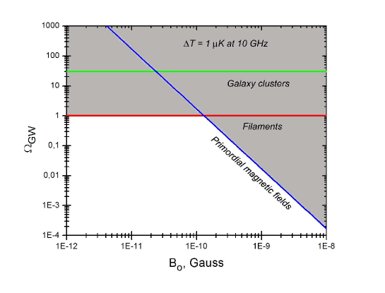
Figure 1: The achievable constraints $\Omega_{GW}$ depending on the strength of the primordial magnetic field $B_{0}$. For comparison the horizontal lines represent the constraints due to magnetic fields in galaxy clusters and filaments. The shaded area indicates the region in parameter space that could be ruled out with current observations. The sensitivity level is set to $1~{}\mu{\rm K}$ at $10~{}{\rm GHz}$ (equivalent to a sensitivity $0.01~{}\mu{\rm K}$ at $100~{}{\rm GHz}$), and a red spatial spectrum for PMF is assumed.

Comparing the observational sensitivity with the expected signal due to HFGWs in the CMB given by (7) in the context of PMF (6), in the absence of a signal, we can place the following constraints on HFGW background

$$\Omega_{GW}\lesssim 1.7\times 10^{-2}\left(\frac{\Delta T_{rms}}{1~{}\mu{\rm K}}\right)\left(\frac{10^{-9}{\rm G}}{B_{0}}\right)^{2}\left(\frac{f}{10^{10}{\rm Hz}}\right)^{2}.$$ (8)

On the other hand, HFGWs with $\Omega_{GW}$ larger than the threshold value (8) would leave an observable signature in the CMB. Note that, the constraints on $\Omega_{GW}$ crucially depend on the strength of the PMF $B_{0}$. For a typical value $B_{0}=10^{-9}~{}\rm{G}$ these constraints are 2-3 orders of magnitude stronger than the analogous constraints due to magnetic fields in galaxy clusters and filaments. In Figure 1 we draw the potential constraints on $\Omega_{GW}$ depending on the strength of the PMF $B_{0}$. The shaded regions represent the regions in $B_{0}$-$\Omega_{GW}$ space that could be potentially ruled out by observations. For comparison, the two horizontal lines show the constraints that arise when considering the magnetic fields in galaxy clusters and filaments.

It is worth noting that in analyzing the potential constraints on $\Omega_{GW}$ through the process of graviton to photon conversion in the presence of magnetic fields we have ignored the inverse process of photon to graviton conversion. This inverse effect has the same probability given by (1). However, at frequencies $f\sim 10^{10}~{}{\rm Hz}$, the energy density of CMB is several orders of magnitude smaller than the typical energy density of HFGW backgrounds considered in this work. For this reason, the total contribution of the inverse effect to changes in the electromagnetic flux remains subdominant.

A potential caveat in our ability to constrain HFGWs arises due to the differential nature of CMB measurements. The conversion probability in presence of PMF is sufficiently isotropic, leading to predominantly isotropic signal in $\Delta T$. The residual anisotropic variations would be $\Delta T_{anis}\sim\Delta T/\sqrt{\eta}=3\times 10^{-3}\Delta T$. A conventional CMB experiment would be restricted to ability to measure only this residual anisotropic variations, weakening the potential constraints on $\Omega_{GW}$. However, PMF produced during inflation with a sufficiently red spatial spectrum Gasperini1995 , may have significantly varying field strength amplitudes in various domains of sub-horizon scale. For these fields the conversion probability would be anisotropic leading to a large anisotropy in the expected signal. On the other hand, this isotropy problem would not arise when considering the CMB signal due graviton conversion in magnetic fields in galaxy clusters and filaments.

A further caveat is also worth mentioning here. In order to detect or constrain the possible signal from HFGWs in the CMB it is necessary to distinguish this signal from other potential mechanisms contributing to the anisotropies in CMB. The commonly considered contributions are the anisotropies due to density perturbations and relic gravitational waves, anisotropies due to Sunyaev-Zel’dovich (SZ) effect, and anisotropies arising due to astrophysical foregrounds PlanckBlueBook . However, these contributions, in general, can be subtracted due to their known frequency dependence. For example, it is known that, the anisotropies due to density perturbations and relic gravitational waves do not depend on frequency (in temperature units, in the Rayleigh-Jeans region). We can estimate the SZ effect in filaments following Rephaeli1995 : $\Delta T_{SZ}\simeq 2Ty\simeq 10^{-2}~{}\mu{\rm K}$ (where $y=\int{dl~{}{\sigma_{T}kT_{e}}n_{e}/mc^{2}}$, and $T_{e}=10^{6}~{}{\rm K}$). This signal has a well understood frequency dependence and for this reason can also be subtracted. Finally, there are indications that the various astrophysical foregrounds, that typically have an amplitude $\Delta T_{foregrd}\sim 10^{2}\mu K$ at $\nu=10^{10}~{}{\rm Hz}$, could be effectively subtracted to a level $\Delta T\lesssim 1~{}\mu\rm{K}$ outside the galactic plane Hinshaw2007 .

Finally, it is useful to compare the sensitivity of the CMB experiments with other methods. The only existing direct measurements of the HFGW background, using laser-interferometeric type detectors, place an upper limit $\Omega_{GW}\lesssim 10^{26}$ in the frequency range around 100 MHz Akutsu2008 . Therefore, it seems highly unlikely that direct measurements would be able to compete with the sensitivity of CMB experiments in the foreseeable future. The most stringent constraint on the possible strength of the HFGW background of cosmological origin are placed by the concordance with the Big-Bang Nucleosynthesis (BBN). This concordance places an upper limit $\Omega_{GW}\lesssim 10^{-5}$ on the total, i.e. integrated over all frequencies, energy of the gravitational wave background (see for example Brustein1996 ). However, this limit assumes that the gravitational wave background was produced prior to the BBN. In contrast, the CMB experiments will also be sensitive to HFGW backgrounds produced at later epochs up to and around the period of recombination. Moreover, CMB experiments can probe the gravitational wave background in a relatively narrow frequency bandwidth around $10^{10}~{}\rm{Hz}$ and are therefore sensitive to sharply peaked HFGW spectra whose total energy might not exceed the BBN limit. In addition, a dedicated CMB experiment could improve sensitivity by 3-4 orders of magnitude, leading to a sensitivity comparable to the BBN limit. In any case, it is worth pointing out that CMB experiments provide an independent technique for observing or constraining HFGWs.

IV Conclusion

In this work, we have analyzed the implications of graviton to photon conversion in the presence of large scale magnetic fields. We have evaluated the conversion probability in the magnetic fields associated with galaxy clusters and filaments as well as primordial magnetic fields. Our estimation imply that this conversion probability is highest for primordial magnetic fields (assuming that PMF have a characteristic strength $B_{0}\sim 10^{-9}~{}{\rm G}$). Assuming realistic values for the magnetic fields, we have shown that a sufficiently strong HFGW background would lead to an observable signature in frequency spectrum of the CMB. We argue that, this signature could be separated from other sources of variations in CMB like the SZ and galactic foregrounds using their corresponding frequency dependences. The current day CMB experiments allow to place significant constraints on the HFGW background ($\Omega_{GW}\lesssim 1$). These limits are about 25 orders of magnitude stronger than existing direct constraints in the high frequency region. Furthermore, these limits could be improved by about 3-4 orders of magnitude in an experiment dedicated to constraining HFGWs.

References

- (1) L. P. Grishchuk, V. M. Lipunov, K. A. Postnov, M. E. Prokhorov and B. S. Sathyaprakash, Usp. Fiz. Nauk 171, 3 (2001) [Sov. Phys. Usp. 44, 1 (2001)].
- (2) C. Cutler and K. S. Thorne, An Overview of Gravitational-Wave Sources, arXiv:gr-qc/0204090.
- (3) B. F. Schutz and B. S. Sathyaprakash, Living Rev. Relativity 12, 2 (2009).
- (4) M. Gasperini and M. Giovannini, Phys. Rev. D 47, 1519 (1993).
- (5) R. Brustein, M. Gasperini, M. Giovannini and G. Veneziano, Phys. Lett. B 361, 45 (1995).
- (6) M. Gasperini and G. Veneziano, Phys. Rep. 373, 1 (2003).
- (7) G. S. Bisnovatiy-Kogan and V. N. Rudenko, Class. Quantum Grav. 21, 3347 (2004).
- (8) L. P. Grishchuk, Discovering Relic Gravitational Waves in Cosmic Microwave Background Radiation, chapter in the “Wheeler Book,” edited by I. Ciufolini and R. Matzner (Springer, New York, to be published), arXiv:0707.3319.
- (9) M. Giovannini, arXiv:0901.3026 (2009)
- (10) C. Clarkson and S. S. Seahra, CQGrav 24, 33 (2007).
- (11) R. Anantua, R. Easther and J. T. Giblin Jr., arXiv:0812.0825 (2008)
- (12) R. Easther, J. T. Giblin Jr. and E. A. Lim, Phys. Rev. Lett. 99, 221301 (2007)
- (13) L. P. Grishchuk and M. V. Sazhin, Sov. Phys. JETP 38, 215 (1974).
- (14) V. B. Braginskii and V. N. Rudenko, Physics Reports 46, 165 (1978).
- (15) L. P. Grishchuk, arXiv:gr-qc/0306013.
- (16) R. M. L. Baker, AIP Conference Proceedings 746, 1306 (2005)
- (17) A. M. Cruise and R. M. J. Ingley, Class. Quantum Grav. 23, 6185 (2006).
- (18) A. Nishizawa et al, Phys. Rev. D 77, 022002 (2008).
- (19) R. M. L. Baker’s Website, http://www.drrobertbaker.com.
- (20) T. Akutsu et al, Phys. Rev. Lett D 101, 101101
- (21) M. E. Gertsenshtein, Sov. Phys. JETP 15, 1, 84 (1962).
- (22) V. B. Braginskii, L. P. Grishchuk, A. G. Doroshkevich, Ya. B. Zel’Dovich, I. D. Novikov, M. V. Sazhin, Sov. Phys. JETP 38, 865 (1974).
- (23) L. P. Grishchuk and A. G. Polnarev, in: General Relativity and Gravitation, 100 Years After the Birth of A. Einstein, edited by A. Held (Plenum Press, NY, 1980), Vol. 2, p. 393.
- (24) Ya. B. Zel’dovich and I. D. Novikov, Relativistic Astrophysics, Vol. 2, The Structure and Evolution of the Universe, Chicago University Press (1983).
- (25) D. Fargion, Gravitation and Cosmology 1, 301 (1995).
- (26) P. P. Kronberg, Rep. Prog. Phys. 57, 325 (1994).
- (27) R. Beck, et al., Annual Rev. Astron. Astrophys. 34, 155 (1996).
- (28) D. Grasso and H. R. Rubinstein, Physics Reports 348, 163 (2001).
- (29) L. M. Widrow, Rev. Mod. Phys. 74, 775 (2002).
- (30) A. Dar and A. de Rujula, Phys. Rev. D 72, 123002 (2005).
- (31) Y. Xu, P. Kronberg, S. Habib and Q. Dufton, Astrophys. J. 637, 19 (2006).
- (32) R. Durrer, New Astron. Rev. 51, 275 (2007).
- (33) M. Giovannini and K. E. Kunze, Phys. Rev. D 77, 061301 (2008).
- (34) J. R. Kristiansen and P. G. Ferreira, Phys. Rev. D 77, 123004 (2008).
- (35) D. G. Yamazaki, K. Ichiki, T. Kajino and G. J. Mathews, Phys. Rev. D 78, 123001 (2008).
- (36) T. Kahniashvili, Yu. Maravin, A. Kosowsky, arXiv:0806.1876 (2008).
- (37) R. Durrer, P. G. Ferreira and T. Kahniashvili, Phys. Rev. D 61, 043001 (2000).
- (38) C. Caprini, R. Durrer, Phys. Rev. D 74, 063521 (2006).
- (39) A. Mack, T. Kahniashvili and A. Kosowsky, Phys. Rev D 65, 123004 (2002).
- (40) A. Lewis, Phys. Rev. D 70, 043011 (2004).
- (41) K. Subramanian, Astronomische Nachrichten 327, 403 (2006).
- (42) A. N. Cillis, D. D. Harari, Phys. Rev. D 54, 4757 (1996)
- (43) P. J. E. Peebles, Principles of Physical Cosmology, (Princeton Un. Press, Princeton, 1993).
- (44) AMI Consortium: J. T. L. Zwart et al. 2008, MNRAS, 391, 1545 (2008)
- (45) Planck Collaboration, The Science Programme of Planck, arXiv:astro-ph/0604069
- (46) M. Gasperini, M. Giovannini, G. Veneziano, Phys. Rev. Lett. 75, 3796 (1995)
- (47) Y. Rephaeli, ApJ 445, 33 (1995)
- (48) G. Hinshaw, et al., Astrophys. J. Supp. 170, 288 (2007).
- (49) R. Brustein, M. Gasperini and G. Veneziano, Phys. Rev. D 55, 3882 (1997).