Casimir Pistons with Curved Boundaries

Abstract

In this paper we study the Casimir force for a piston configuration in $R^{3}$ with one dimension being slightly curved and the other two infinite. We work for two different cases with this setup. In the first, the piston is ”free to move” along a transverse dimension to the curved one and in the other case the piston ”moves” along the curved one. We find that the Casimir force has opposite signs in the two cases. We also use a semi-analytic method to study the Casimir energy and force. In addition we discuss some topics for the aforementioned piston configuration in $R^{3}$ and for possible modifications from extra dimensional manifolds.

Introduction

More than 60 years have passed since H. Casimir’s [1] originating paper, stating that there exist’s an attractive force between two neutral parallel conducting plates. After 20 years, the scientific society had appreciated this work and extended this work in various areas, from solid state physics to quantum field theory and even cosmology [13, 14, 11]. The Casimir effect is closely related with the existence of zero point quantum oscillations of the electromagnetic field in the case of parallel conducting plates. The boundaries polarize the vacuum and that results to a force acting on the boundary [11]. The Casimir force can be either repulsive or attractive. That dependents on the nature of the background field in the vacuum, the geometry of the boundary, the dimension and the curvature of the spacetime. The regularization of the Casimir energy is of particular important in order physical results become clearer.

One very interesting configuration is the so called Casimir piston. This configuration was originally treated [9] as a single rectangular box with three parallel plates. The one in the middle is the piston. The dimensions of the piston are $(L-a)\times b$ and $a\times b$, with the piston being located in $a$. In [9] the Casimir energy and Casimir force for a scalar field was calculated. The boundary conditions on the ’plates’ where Dirichlet. There exists a large literature on the subject [8, 25, 27, 26, 7, 3, 2, 10, 16, 17, 18, 19] calculating the Casimir force for various piston configurations and for various boundary conditions of the scalar field. Also most results where checked at finite temperature. The configurations used where extended to include extra dimensional spaces which form a product spacetime with the piston topology, that is $M_{Piston}\times M^{n}$, with $M_{Piston}$ and $M^{n}$ the piston spacetime topology and the extra dimensional spacetime topology. In addition to the known Neumann and Dirichlet boundary conditions, in reference [7] Robin boundary conditions where considered for a Kaluza-Klein piston configuration. In most cases the scalar field was taken massless but there exists also literature for the massive case [28].

The calculational advantage the Casimir piston provides is profound. Particularly, when one calculates the Casimir energy between parallel plates confronts infinities that must be regularized. The regularization of the Casimir energy in the parallel plate geometry can be done if we calculate it as a sum over discrete modes (due to boundary conditions on the plates) minus the continuum integral (with no plates posing boundary conditions)[11, 13, 14]. The discrete sum consists of three parts, a volume divergent term (which be cancelled by the continuum integral), a surface divergent term and a finite part. This can be easily seen if the calculations of the Casimir energy are done with the introduction of a UV cutoff, $\lambda$. Before the piston setup was firstly used, the surface divergent term was thrown out. Actually this was proven to be completely wrong because such surface divergent term cannot be removed by renormalization of the physical parameters of the theory [31]. The zeta regularization technique renormalizes this term to zero. Thus the cutoff technique and the zeta regularization technique agree perfectly. However there is no reason to justify the loss of the surface term within the cutoff regularization technique. The Casimir piston solves this problem in a very nice way, because the surface terms of the two piston chambers cancel and thus the Casimir force can be consistently calculated [8, 25, 27, 26, 7, 3, 2, 10, 16, 17, 18, 19]. We shall use the zeta-function regularization technique and also treat the problem numerically. Also in the last section we shall briefly give the expression of the Casimir energy using a cutoff regularization technique and demonstrate how the surface terms cancel.

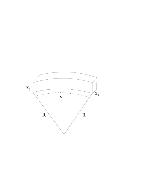
Figure 1: Curved Piston Configuration with Infinite Radius

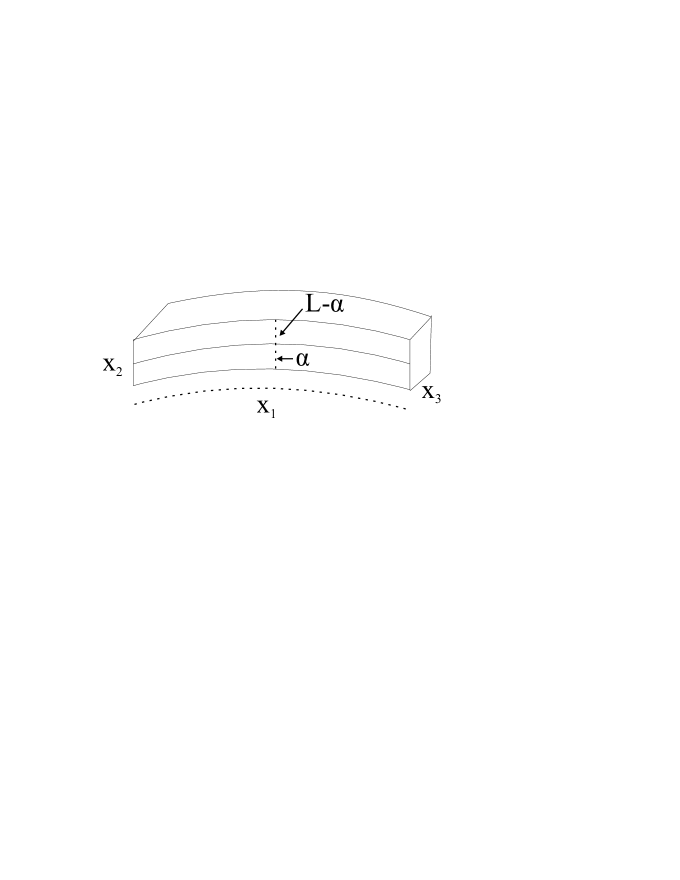
Figure 2: Piston 1, The moving piston along the non-curved dimension $x_{2}$

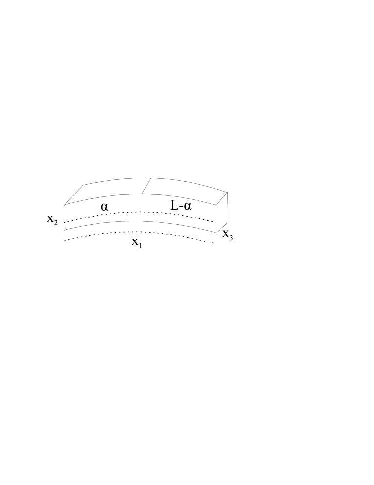
Figure 3: Piston 2, The moving piston along the curved dimension $x_{1}$

Motivated by a recent paper [2], we shall consider a piston configuration in $R^{3}$ space without the extra dimensions. In this topology we consider a piston geometry living in three space. We shall study two configurations which can be seen in Figures 2 and 3. In the first case Fig. 2, the $x_{1}$ and $x_{3}$ dimensions are sent to infinity and we have ”parallel plates” having distance $\L$ between them. The piston consists of two such three dimensional chambers with the piston plate having distance $\alpha$ and $L-\alpha$ from the boundary plates. In addition to this we shall assume that in one of the two infinite dimensions, there is curvature. As can be seen the infinite dimension $x_{1}$ seems to be a part of a circle. We shall work in the case where the radius of the circle goes to infinity, that is when $R\rightarrow\infty$. We shall give the solution for the Laplace equation for a scalar field (with Dirichlet boundary conditions at all boundaries, see below) corresponding to this configuration and find the eigenfrequencies. Next we calculate the Casimir energy and the Casimir force for each chamber and for the whole configuration using standard techniques [11, 13, 14]. Additionally we study a similar to the above situation, described by Figure 3. Particularly in this case the piston is free to move along the curved dimension and $x_{2}$ and $x_{3}$ are infinite dimensions. These cases shall be presented in section 1. In section 2 we discuss the results we found in section 1. In section 3 we present a semi-analytic calculation of the Casimir energy and Casimir force. Finally the conclusions with a discussion follow.

Before closing this section it worths discussing what is the motivation to study scalar field Casimir energy (and closely connected to this, the Casimir piston configurations) and particularly at four spacetime dimensions, that is 3+1, 3 space and one time. The studies of Casimir effect in higher dimensions through the effective action calculation [4, 5, 6] are very interesting especially when vacuum stability issues are addressed. Pistons including extra dimensions serve in defining the impact of extra dimensions in an observable way. So why studying pistons in 3+1 dimensions? The first reason comes from studies of Bose-Einstein condensates [21, 22, 23]. Particularly when calculating the Casimir energy and pressure in a zero temperature homogeneous weakly interacting dilute Bose-Einstein condensate in a parallel plate geometry including Bogoliubov corrections, the leading order term is identified with the Casimir energy of a massless scalar field [21, 22, 23]. This fact begins a new era in experiments because the scalar field Casimir force can be measured in Bose-Einstein condensates. This will be the first thing to measure actually, because the leading order term is the scalar Casimir force. In connection with these, the Bose-Einstein condensates have very interesting prospects. Particularly, Bose-Einstein condensates are known to provide an effective metric and for mimicking kinematic aspects of general relativity, thus probing kinematic aspects of general relativity [21, 22, 23].

Another motivation for studying scalar Casimir energies in 3+1 dimensions is the connection of the scalar Casimir energy with the electromagnetic field Casimir energy in 3+1 dimensions [15] and also the 4-dimensional perfect conductor Casimir energy of the electromagnetic field is identical with the 3-dimensional scalar field Casimir energy by dimensional reduction [24]. Let us discuss on these two in detail. The Casimir energy of an electromagnetic field in the radiation gauge is connected with the Dirichlet massless scalar field Casimir energy with the general relation (see for example Ambjorn and Wolfram [15]),

$$E_{A}(a_{1},a_{2},..,a_{p};p;d)=(d-1)E_{\phi_{D}}(a_{1},a_{2},..a_{p};p;d)+\sum_{i=1}^{p}E_{\phi_{D}}(a_{1},a_{2},..a_{i-1},a_{i+1},...,a_{p};p-1;d-1)$$ (1)

In the above equation, $p$ and $d$ are the dimensions of a a hypercuboidal region with p sides of finite length $a_{1},a_{2},..a_{p}$ and $d-p$ sides with length $L\gg a_{i}$, ($i=1,2,..p$).

Of course the electromagnetic field Casimir force calculations are most valuable in the case of nano devices, where attractive Casimir forces may cause the collapse of the device. This is known as stiction [21, 22, 23, 25, 27, 26].

One strong motivation to study scalar and electromagnetic Casimir energies in various topologies and geometries comes from the fact that the scalar and electromagnetic Casimir energies are maybe connected quantitatively within the piston setup. In a recent study, A. Edery et.al [24] studied exactly this issue. Let us discuss some of their results relevant to us. The authors found that the original Cavalcanti’s 2+1 dimensional scalar Dirichlet Casimir piston can be obtained by dimensionally reducing a 3+1 dimensional electromagnetic piston system obeying perfect conductor conditions. This novel observation serves to open new directions in studying various piston configurations in 3+1 dimensions. Having in mind that the electromagnetic Casimir energy is closely related to the Dirichlet scalar Casimir energy [15], this can be proven really valuable. We must mention that as proved by the authors of [24], this happens only for 3+1 dimensional electromagnetic piston systems. This makes 3+1 dimensional piston studies really interesting both theoretically and maybe at some point experimentally, for example in nano devices where the boundaries form the various topologies. We have to mention that the dimensional reduction as worked out by the authors of [24] does not refer to the reduction of a toroidal dimension but to the reduction of an interval (for example $(0,L)$) with boundary conditions that respect the symmetries of the original action (perfect electric conductor). The reduction is obtained by setting the interval length go to zero, that is $L\rightarrow 0$. They studied the general case with $d$ dimensions. In general the dimensional reduction (as in the compact dimensions case) leads to a massive tower of massive Kaluza-Klein states with mass inverse proportional to $L^{2}$. When $L\rightarrow 0$ these states decouple from the theory only when the original electromagnetic system leaves in 3+1 dimensions. The initial search was to see whether a $d$ dimensional electromagnetic field reduces to the $d-1$ electromagnetic field after dimensional reduction. They found that for three dimensions the electromagnetic field has one degree of freedom and also the scalar field has one degree of freedom. Thus as long the boundary conditions match, these two can be considered equivalent. Particularly the Casimir force is identical in the two cases (see [24] for many details and the proof). This is a valuable result both theoretically and experimentally. Experimentally because this reduction scenario could be investigated in high precision Casimir experiments with real metals in 3 space dimensions (3+1 spacetime)

An additional theoretical prospect of the dimensional reduction setup of reference [24] is the similarity of the whole configuration with orbifold boundary conditions. We shall not discuss on this now but we hope to comment soon.

In addition, another result found in paper [24] is that the reduction of a $d$ dimensional Dirichlet scalar Casimir piston does not lead to the $d-1$ dimensional scalar Casimir piston. Actually under the reduction, the Casimir energy goes to zero. This is intriguing showing us that the close relation of electromagnetic 3+1 pistons with 2+1 scalar pistons is really valuable. Regarding the $d$-dimensional scalar and it’s relation with the $d-1$ scalar theory there is a well known relation between the two through finite temperature field theory [34]. Specifically a theory at finite temperature offers the possibility to connect a $d-1$ dimensional scalar theory with the $d$ dimensional theory at finite temperature. However we must be really cautious because the argument that a $d$ dimensional field theory correspond to the same theory in $d-1$ dimensions has been proven true [34] only for the $\phi^{4}$ theory (always within the limits of perturbation theory). Also this also holds true for supersymmetric theories. On the contrary this does not hold for $QCD$ and Yang-Mills theories. Actually $QCD_{3}$ resembles more $QCD_{4}$ and not $QCD_{4}$ at finite temperature. Following these lines it would be interesting to see whether this argument holds for the scalar Casimir pistons with various boundary conditions, that is to check whether the 3+1 dimensional scalar Casimir piston force at finite temperature is equal to the 2+1 Casimir piston, in the infinite temperature limit. Also there exists an argument stating that a $d$ dimensional theory at finite temperature resembles more the same theory with one dimension compactified to a circle and in the limit $R\rightarrow 0$, where $R$ the magnitude of the compact dimension. It would be interesting to examine this within the Edery’s [24] dimensional reduction scheme.

Finally a motivation to study the piston configuration we use in this paper is the asymmetry that one of the two piston we use has. Particularly the figure 2 configuration. There exists an argument in the literature stating that the Casimir force between bodies related by reflection is always attractive, independent of the exact form of the bodies or dielectric properties. As we will see in the following this argument applies both to the two cases we use, thus proving that a small deviation from the reflection symmetry does not modify the standard results of rectangular pistons.

1 The Piston Setup

The configuration of Figure 2 can be described as follows: The curvature of the infinite length curved dimension is $\frac{1}{R}$ and the width between plates is $\alpha$ and $L-\alpha$ for the two chambers. We shall treat only the $\alpha$ chamber first. The generalization to the other case is straightforward. In order to describe this slightly curved piston setup more efficiently, we choose the coordinates $s,t$ to describe the plane $x_{1}-x_{2}$ and $x_{3}$ remains the same, as it appears in Figure 2. The piston is based on the papers [29, 30]. We borrowed the analysis and the ansatz solutions that the authors used for bent waveguides. Following [29, 30], the local element in the plane $s-t$ is $\mathrm{d}A=h(s,t)\mathrm{d}s\mathrm{d}t$, with $s$ the length along the infinite slightly curved dimension and $t$ the transverse dimension, with $h(s,t)=1-\frac{1}{R}t$. The Laplacian in terms of $s,t,x_{3}$ looks like (acting on $\psi$, with $\psi$ a scalar field),

$$\nabla^{2}\psi=\frac{1}{h}\frac{\partial}{\partial t}(h\frac{\partial\psi}{\partial t})+\frac{1}{h}\frac{\partial}{\partial s}(h\frac{\partial\psi}{\partial s})+\frac{\partial^{2}\psi}{\partial x_{3}^{2}}.$$ (2)

If in the above relation we expand $h(s,t)$ for $R\rightarrow\infty$, then the non-vanishing terms in first order approximation yield the usual Laplacian in Cartesian coordinates. An ansatz solution of $\nabla^{2}\psi=0$ is:

$$\psi(s,t,x_{3})=\frac{u(s)}{\sqrt{h(s,t)}}\sin{(\frac{n\pi t}{\alpha})}e^{ik_{3}{\,}x_{3}},$$ (3)

subject to the Dirichlet boundary conditions, $\psi(s,t,x_{3})=\psi(s,t+\alpha,x_{3})=0$ for the transverse coordinate $t$. Relation (3) for infinite $R$ yields (keeping first order non vanishing terms):

$$\psi(s,t,x_{3})=u(s)\sin{\frac{n\pi t}{\alpha}}e^{ik_{3}{\,}x_{3}},$$ (4)

with $u(s)$ satisfying:

$$\frac{\mathrm{d}^{2}u}{\mathrm{ds}^{2}}+(k^{2}-\frac{\pi^{2}}{\alpha^{2}}+\frac{1}{R^{2}})u(s)=0.$$ (5)

Then the eigenfrequencies of the above configuration is,

$$\omega^{2}=k^{2}_{1}+k_{2}^{2}+(\frac{n\pi}{\alpha})^{2}-\frac{\pi^{2}}{\alpha^{2}}+\frac{1}{R^{2}}.$$ (6)

Notice that in the limit $R\rightarrow\infty$, the term $-\frac{\pi^{2}}{\alpha^{2}}+\frac{1}{R^{2}}$ is negative. In the next section we shall comment on this.

Now the Casimir energy per unit area for the chamber with transverse length $\alpha$ is [11] (bearing in mind that $-\frac{\pi^{2}}{\alpha^{2}}+\frac{1}{R^{2}}$ is much less than $1$):

$$E_{ren}(\alpha)=$$ (7)

$$\int_{-\infty}^{\infty}\frac{\mathrm{d}k_{1}\mathrm{d}k_{2}}{4\pi^{2}}\Big{(}\sum_{n=1}^{\infty}\sqrt{k^{2}_{1}+k_{2}^{2}+(\frac{n\pi}{\alpha})^{2}-\frac{\pi^{2}}{\alpha^{2}}+\frac{1}{R^{2}}}$$

$$-\frac{a}{\pi}\int_{\sqrt{-\frac{1}{R^{2}}+\frac{\pi^{2}}{\alpha^{2}}}}^{\infty}\sqrt{k^{2}_{1}+k_{2}^{2}+(\frac{n\pi}{\alpha})^{2}-\frac{\pi^{2}}{\alpha^{2}}+\frac{1}{R^{2}}}\Big{)},$$

where the left term is the finite $\alpha$ part and the right term the infinite $\alpha$ part. The substraction of the continuum part from the finite part corrections is a very well known renormalization technique for the Casimir energy [11]. Now, performing the $k_{1}$, $k_{2}$ integration, one obtains:

$$E_{ren}(\alpha)=$$ (8)

$$\frac{3}{2\pi}\Big{(}\sum_{n=1}^{\infty}\big{[}(\frac{n\pi}{\alpha})^{2}-\frac{\pi^{2}}{\alpha^{2}}+\frac{1}{R^{2}}\big{]}^{3/2}-\frac{a}{\pi}\int_{\sqrt{-\frac{1}{R^{2}}+\frac{\pi^{2}}{\alpha^{2}}}}^{\infty}\big{[}(\frac{n\pi}{\alpha})^{2}-\frac{\pi^{2}}{\alpha^{2}}+\frac{1}{R^{2}}\big{]}^{3/2}\Big{)}.$$

The $k_{1}$, $k_{2}$ integration is done using,

$$\int\mathrm{d}k_{1}\mathrm{d}k_{2}\sum_{n=1}^{\infty}\big{[}k_{1}^{2}+k_{2}^{2}+\big{(}\frac{n\pi}{a}\big{)}^{2}-m^{2}\big{]}^{-s},$$ (9)

which after integrating over $k_{1}$ and $k_{2}$ we obtain,

$$\Gamma(s-1){\,}\pi\sum_{n=1}^{\infty}\big{[}\big{(}\frac{n\pi}{a}\big{)}^{2}-m^{2}\big{]}^{1-s}.$$ (10)

Analytically continuing the above to $s=-\frac{1}{2}$ we obtain relation (8). Upon using the Abel-Plana formula [11, 12],

$$\sum_{n=0}^{\infty}f(n)-\int_{0}^{\infty}f(n)\mathrm{d}n=\frac{1}{2}f(0)+i\int_{0}^{\infty}\mathrm{d}t\frac{f(it)-f(-it)}{e^{2\pi t}-1},$$ (11)

the Casimir energy (8) becomes,

$$E_{ren}(\alpha)=\frac{3}{2\alpha}\Big{(}\frac{1}{2}(1-b^{2})^{3/2}$$ (12)

$$-\int_{0}^{\infty}\mathrm{d}t\frac{1}{e^{2\pi t}-1}\Big{[}2t\sqrt{\frac{\sqrt{(1-b^{2}-t^{2})^{2}+4t^{2}}+1-b^{2}-t^{2}}{2}}$$

$$+(1-b^{2}-t^{2})\sqrt{\frac{\sqrt{(1-b^{2}-t^{2})^{2}+4t^{2}}-1+b^{2}+t^{2}}{2}}\Big{]}$$

$$+\frac{1}{8}\big{(}(5b^{2}-2)\sqrt{-b^{2}+1}+3b^{4}(\ln b-\ln(1+\sqrt{1-b^{2}}))\big{)}\Big{)},$$

with

$$b=\frac{\alpha\sqrt{-\frac{1}{R^{2}}+\frac{\pi^{2}}{\alpha^{2}}}}{\pi}.$$ (13)

Following the same steps us above, with $a\rightarrow L-\alpha$, we obtain the renormalized Casimir energy for the chamber $L-\alpha$:

$$E_{ren}(L-\alpha)=\frac{3}{2(L-\alpha)}\Big{(}\frac{1}{2}(1-\lambda^{2})^{3/2}$$ (14)

$$-\int_{0}^{\infty}\mathrm{d}t\frac{1}{e^{2\pi t}-1}\Big{[}2t\sqrt{\frac{\sqrt{(1-\lambda^{2}-t^{2})^{2}+4t^{2}}+1-\lambda^{2}-t^{2}}{2}}$$

$$+(1-\lambda^{2}-t^{2})\sqrt{\frac{\sqrt{(1-\lambda^{2}-t^{2})^{2}+4t^{2}}-1+\lambda^{2}+t^{2}}{2}}\Big{]}$$

$$+\frac{1}{8}\big{(}(5\lambda^{2}-2)\sqrt{-\lambda^{2}+1}+3\lambda^{4}(\ln\lambda-\ln(1+\sqrt{1-\lambda^{2}}{\,}))\big{)}\Big{)},$$

and for this case

$$\lambda=\frac{(L-\alpha)\sqrt{-\frac{1}{R^{2}}+\frac{\pi^{2}}{(L-\alpha)^{2}}}}{\pi}.$$ (15)

Now the total Casimir energy for the piston is obtained by adding relations (12) and (14), namely,

$$E_{Piston}=E_{ren}(L-\alpha)+E_{ren}(\alpha).$$ (16)

In Figures 4, 5 and we plot the Casimir energy for the chamber $\alpha$, $L-\alpha$ respectively, for the numerical values $R=10^{100}$, $L=10^{11}$. Also in Figures 6, 7 and 8 we plot the Casimir force for the chambers $\alpha$, $L-\alpha$ and the total Casimir force, respectively.

Figure 4: The Casimir Energy for the chamber $\alpha$, for $R=10^{100}$, $L=10^{11}$ (Piston 1 Case)

Figure 5: The Casimir Energy for the chamber $L-\alpha$, for $R=10^{100}$, $L=10^{11}$ (Piston 1 Case)

Figure 6: The Casimir Force for the chamber $\alpha$, for $R=10^{100}$, $L=10^{11}$ (Piston 1 Case)

Figure 7: The Casimir Force for the chamber $L-\alpha$, for $R=10^{100}$, $L=10^{11}$ (Piston 1 Case)

Figure 8: The total Piston Casimir Force, for $R=10^{100}$, $L=10^{11}$ (Piston 1 Case)

1.1 Another Piston Configuration

Let us now study the case for the piston configuration appearing in Figure 3. Following the previous steps, the eigenvalue spectrum of the Laplacian is:

$$\omega^{2}=k^{2}_{1}+k_{2}^{2}+(\frac{n\pi}{\alpha})^{2}-\frac{1}{R^{2}}.$$ (17)

Now the Casimir energy for the $\alpha$ piston is (after integrating on the infinite dimensions),

$$E_{ren}(\alpha)=$$ (18)

$$\frac{3}{2\pi}\Big{(}\sum_{n=1}^{\infty}\big{[}(\frac{n\pi}{\alpha})^{2}-\frac{1}{R^{2}}\big{]}^{3/2}-\frac{a}{\pi}\int_{\frac{1}{R}}^{\infty}\big{[}(\frac{n\pi}{\alpha})^{2}-\frac{1}{R^{2}}\big{]}^{3/2}\Big{)}.$$

Upon using again the Abel-Plana formula [11, 12], the Casimir energy (18) becomes,

$$E_{ren}(\alpha)=\frac{3}{2\alpha}\Big{(}\frac{1}{2}(1-b^{2})^{3/2}$$ (19)

$$-\int_{0}^{\infty}\mathrm{d}t\frac{1}{e^{2\pi t}-1}\Big{[}2t\sqrt{\frac{\sqrt{(1-b^{2}-t^{2})^{2}+4t^{2}}+1-b^{2}-t^{2}}{2}}$$

$$+(1-b^{2}-t^{2})\sqrt{\frac{\sqrt{(1-b^{2}-t^{2})^{2}+4t^{2}}-1+b^{2}+t^{2}}{2}}\Big{]}$$

$$+\frac{1}{8}\big{(}(5b^{2}-2)\sqrt{-b^{2}+1}+3b^{4}(\ln b-\ln(1+\sqrt{1-b^{2}}))\big{)}\Big{)},$$

with

$$b=\frac{\alpha}{R\pi}.$$ (20)

Following the same steps us above, with $a\rightarrow L-\alpha$, we obtain the renormalized Casimir energy for the chamber $L-\alpha$:

$$E_{ren}(L-\alpha)=\frac{3}{2(L-\alpha)}\Big{(}\frac{1}{2}(1-\lambda^{2})^{3/2}$$ (21)

$$-\int_{0}^{\infty}\mathrm{d}t\frac{1}{e^{2\pi t}-1}\Big{[}2t\sqrt{\frac{\sqrt{(1-\lambda^{2}-t^{2})^{2}+4t^{2}}+1-\lambda^{2}-t^{2}}{2}}$$

$$+(1-\lambda^{2}-t^{2})\sqrt{\frac{\sqrt{(1-\lambda^{2}-t^{2})^{2}+4t^{2}}-1+\lambda^{2}+t^{2}}{2}}\Big{]}$$

$$+\frac{1}{8}\big{(}(5\lambda^{2}-2)\sqrt{-\lambda^{2}+1}+3\lambda^{4}(\ln\lambda-\ln(1+\sqrt{1-\lambda^{2}}))\big{)}\Big{)},$$

and for this case

$$\lambda=\frac{(L-\alpha)}{R\pi}.$$ (22)

Now the total Casimir energy for the piston is obtained by adding relations (19) and (21), namely,

$$E_{Piston}=E_{ren}(L-\alpha)+E_{ren}(\alpha).$$ (23)

In Figures 9 we plot the Casimir energy for the chamber $\alpha$ and for the numerical values $R=10^{100}$, $L=10^{11}$. Also in Figures 10, 11 and 13 we plot the Casimir force for the chamber $\alpha$ the chamber $L-\alpha$ and the total Casimir force.

Figure 9: The Casimir Energy for the chamber $\alpha$, for $R=10^{100}$, $L=10^{11}$ (Piston 2 Case)

Figure 10: The Casimir Force for the chamber $\alpha$, for $R=10^{100}$, $L=10^{11}$ (Piston 2 Case)

Figure 11: The Casimir Force for the chamber $L-\alpha$, for $R=10^{100}$, $L=10^{11}$ (Piston 2 Case)

Figure 12: The total Piston Casimir Force, for $R=10^{100}$, $L=10^{11}$ (Piston 2 Case)

Figure 13: The total Piston Casimir Force, for $R=10^{100}$, $L=10^{11}$ and for a wide range of $\alpha$ (Piston 2 Case)

2 Brief Discussion

Let us discuss the results of the previous section. We start with the piston 1 that appears in Figure 2. The Casimir force that stems out of this configuration is described by Figures 6, 7 and 8. As it can be seen, the total Casimir force is negative for small $\alpha$. Also for large $\alpha$, for values near $L$, the total Casimir energy is positive. In conclusion the Casimir force is attractive when the piston is near to the one end. In addition it is repulsive if the piston goes to the other end. This kind of behavior is a known result for pistons (see [2]). Remember this case corresponds to a piston that is ”free to move” along one of the non curved dimensions.

In the case of Piston 2 of Figure 3 the results are different. Now the piston is ”free to move” along the slightly curved dimension of total length $L$. This case is best described by Figures 10, 11 and 13. As we can see, the total Casimir force is positive for small $\alpha$ values and negative for large $\alpha$ values (but still smaller than $L$). This means that the Casimir force is repulsive to the one end and attractive to the other one. Note that this behavior is similar to the Piston 1 case with the difference that the force is attractive (repulsive) to different places. However the qualitative behavior that is described by repulsion to one end and attraction to the other, still holds. In the next section we shall verify this using a semi-analytic approximation.

3 A Semi-analytic Approach for the Piston Casimir Energy and Casimir Force

In this section we shall consider as in previous sections a three dimensional piston $R^{3}$ and for simplicity the piston of Figure 3. Our study will be focused on the semi-analytic calculation of the Casimir energy and Casimir force.

The piston configuration consists of two chambers with lengths $\alpha$ and $L-\alpha$, and with Dirichlet boundary conditions on the boundaries and on the moving piston. The energy eigenfrequency for this setup is:

$$\omega^{2}=k^{2}_{1}+k_{2}^{2}+(\frac{n\pi}{\alpha})^{2}-y^{2},$$ (24)

for the $\alpha$ chamber, and

$$\omega^{2}=k^{2}_{1}+k_{2}^{2}+(\frac{n\pi}{L-\alpha})^{2}-y^{2},$$ (25)

for the $L-\alpha$ chamber. In the above two relations the parameter $y$ stands for a positive number with physical significance analogous to the ones we described in the previous sections. The Casimir energy with no regularization for this system is given by:

$$E_{Piston}=E_{P}(L-\alpha)+E_{P}(\alpha),$$ (26)

where $E_{P}(\alpha)$ is (upon integrating the infinite dimensions):

$$E_{P}(\alpha)=\frac{3}{2\pi}\sum_{n=1}^{\infty}\Big{[}\big{(}\frac{n\pi}{\alpha}\big{)}^{2}-y^{2}\Big{]}^{3/2}.$$ (27)

As we said, the above sum contains a singularity and needs regularization. In order to see how the singularity ”behaves” we use the binomial expansion (or a Taylor expansion for small $y$, which is exactly the same as can be checked):

$$(a^{2}-b^{2})^{s}=\sum_{l=0}^{\sigma}\frac{s!}{(s-l)!l!}(a^{2})^{l}(-b^{2})^{s-l},$$ (28)

and rearranging the sum as:

$$E_{P}(\alpha)=\frac{3\pi^{2}}{2\alpha^{3}}\sum_{n=1}^{\infty}(n^{2}-m^{2})^{3/2},$$ (29)

and $m=\frac{y\alpha}{\pi}$ we obtain:

$$E_{P}(\alpha)= \sum_{n=1}^{\infty}\frac{3}{2\pi}\Big{(}\frac{n^{3}}{\alpha^{3}}-\frac{3y^{2}n}{2\alpha\pi^{2}}+\frac{3\alpha y^{4}}{8n\pi^{4}}+\frac{\alpha^{3}y^{6}}{16n^{3}\pi^{6}}$$ (30)

$$+\frac{3\alpha^{5}y^{6}}{128n^{5}\pi^{8}}+\frac{3\alpha^{7}y^{10}}{256n^{7}\pi^{10}}+\frac{7\alpha^{9}y^{1}2}{1024n^{9}\pi^{1}2}...\Big{)}.$$

Using the zeta regularization method [13, 14] the above relation (30) becomes,

$$E_{P}(\alpha)= \frac{3}{2\pi}\Big{(}\frac{\zeta(-3)}{\alpha^{3}}-\frac{3y^{2}\zeta(-1)}{2\alpha\pi^{2}}+\frac{3\alpha y^{4}\zeta(1)}{8\pi^{4}}+\frac{\alpha^{3}y^{6}\zeta(3)}{16\pi^{6}}$$ (31)

$$+\frac{3\alpha^{5}y^{6}\zeta(5)}{128\pi^{8}}+\frac{3\alpha^{7}y^{10}\zeta(7)}{256\pi^{10}}+\frac{7\alpha^{9}y^{12}\zeta(9)}{1024\pi^{12}}...\Big{)}.$$

Notice that the singularity is contained in $\zeta(1)$ and is a pole of first order. Now the other chamber of the piston contributes to the Casimir energy as:

$$E_{P}(L-\alpha)= \frac{3}{2\pi}\Big{(}\frac{\zeta(-3)}{(L-\alpha)^{3}}-\frac{3y^{2}\zeta(-1)}{2(L-\alpha)\pi^{2}}+\frac{3(L-\alpha)y^{4}\zeta(1)}{8\pi^{4}}+\frac{(L-\alpha)^{3}y^{6}\zeta(3)}{16\pi^{6}}$$ (32)

$$+\frac{3(L-\alpha)^{5}y^{6}\zeta(5)}{128\pi^{8}}+\frac{3(L-\alpha)^{7}y^{10}\zeta(7)}{256\pi^{10}}+\frac{7(L-\alpha)^{9}y^{12}\zeta(9)}{1024\pi^{12}}...\Big{)}.$$

Before proceeding we must mention that we could reach the same results as above by Taylor expanding the initial sum of relation (27) for $y\rightarrow 0$.

Let us now discuss the above. It can be easily seen that the total Casimir force,

$$F_{c}=-\frac{\partial E_{P}(L-\alpha)}{\partial\alpha}-\frac{\partial E_{P}(\alpha)}{\partial\alpha},$$ (33)

is free or singularity. The reason is obvious and it is because the pole containing term is linear to the length of the piston chamber. Due to this linearity, the derivative of the energy cancels this dependence and the two singularities cancel each other. Thus we see how in our case also, a slightly curved piston configuration results to a singularity free Casimir force.

Finally, let us discuss something different. One quantity that is also free of singularity is,

$$N(\alpha)=\frac{E_{P}(\alpha)}{\alpha}-\frac{E_{P}(L-\alpha)}{L-\alpha}.$$ (34)

It is not accidental that this quantity has dimensions Energy per length which is actually force. The finiteness of the piston Casimir force and the force related quantity $N(\alpha)$ show once more, as is well known [9, 2], that the piston configuration has many attractive field theoretic features, even in the presence of very small curvature in one of the dimensions. The same arguments hold regarding the quantity (34), also when we consider a massive scalar field in an usual $R^{3}$ piston configuration (with no curved dimensions).

3.1 Semi-analytic Analysis for the Piston Casimir Force

According to the above, the Casimir energy can be approximated by relations (31) and (32). Thus when the radius of the slightly curved dimension is very large, the Casimir force can be approximated by,

$$F_{c}(\alpha)=-\frac{9\pi\zeta(-3)}{\alpha^{4}}+\frac{9y^{2}\zeta{(-1)}}{2\alpha^{2}\pi}+\frac{9\alpha^{2}y^{6}\zeta{(3)}}{16\pi^{5}},$$ (35)

for the chamber $\alpha$, and

$$F_{c}(L-\alpha)=-\frac{9\pi\zeta(-3)}{(L-\alpha)^{4}}+\frac{9y^{2}\zeta{(-1)}}{2\alpha^{2}\pi}+\frac{9(L-\alpha)^{2}y^{6}\zeta{(3)}}{16\pi^{5}},$$ (36)

for the $L-\alpha$ chamber. When $R$ is much larger than $\alpha$, (with $y=1/R$) then the approximation we used above is adequate to describe the Casimir force. In Figures 14, 15 and 16, we plot the Casimir force for the chamber $\alpha$, $L-\alpha$ and the total force, for $R=10^{20}$ and $L=10^{11}$

Figure 14: The Casimir Force for the chamber $\alpha$, for $R=10^{20}$, $L=10^{11}$ (Piston 2 Case)

Figure 15: The total Piston Casimir Force, for $R=10^{20}$, $L=10^{11}$ (Piston 2 Case)

Figure 16: The total Piston Casimir Force, for $R=10^{20}$, $L=10^{11}$ and for a wide range of $\alpha$ (Piston 2 Case)

As it can be seen from the Figures, the behavior of the Casimir force is the same as the one we found in section 1. Thus for the Piston 2 configuration, the Casimir force is positive for the $\alpha$ chamber and negative for the $L-a$ chamber (when $\alpha$ approaches the size of $L$). Also the total Casimir force is positive for small $\alpha$ and negative for large $\alpha$.

A similar analysis can be carried for the Piston 1 configuration and similar results hold.

Finally we plot the quantity $N(\alpha)$ of relation (34). In Figure 17 we can see that the behavior of $N(\alpha)$ resembles that of the total Casimir force we studied previously, for the case of Piston 2, and for the $\alpha$ chamber.

Figure 17: The quantity $N(\alpha)$, for $R=10^{100}$, $L=10^{12}$ and for a wide range of $\alpha$ (Piston 2 Case)

Before closing this section let us briefly comment on the regularization dependence of the force corresponding to the pistons we used. We shall make use of a cutoff parameter $\lambda$ in the Casimir energy, in order to see explicitly the cancellation of the surface terms we mentioned in the introduction [11, 25, 27, 26, 16, 17, 18, 19]. We work again for the piston 2 configuration. The Casimir energy for the $a$ chamber is [25, 27, 26],

$$E^{P}_{Cas}(\lambda,a,y)=\frac{1}{2}\sum_{n=1}^{\infty}\frac{3}{2\pi}\Big{[}\big{(}\frac{n\pi}{\alpha}\big{)}^{2}-y^{2}\Big{]}^{3/2}e^{-\lambda\Big{[}\big{(}\frac{n\pi}{\alpha}\big{)}^{2}-y^{2}\Big{]}^{3/2}}$$ (37)

The finite Casimir energy is obtained by taking the limit $\lambda\rightarrow 0$ in the regular term of the Casimir energy (we will see it shortly). After using the inverse Mellin transform [25, 27, 26] of the exponential and observing that,

$$E^{P}_{Cas}(\lambda,a,y)=-\frac{3}{2}\frac{\partial}{\partial\lambda}\sum_{n=1}^{\infty}e^{-\lambda\Big{[}\big{(}\frac{n\pi}{\alpha}\big{)}^{2}-y^{2}\Big{]}^{3/2}}$$ (38)

we obtain (following the technique of reference [25, 27, 26]),

$$E^{P}_{Cas}(\lambda,a,y)=a\frac{3}{2\pi\lambda^{2}}+\frac{3{\,}y^{2}{\,}a}{4\pi}\log\lambda+E_{\mathrm{regular}}(a)$$ (39)

for the $a$ chamber, while for the $L-a$ chamber we obtain accordingly,

$$E^{P}_{Cas}(\lambda,L-a,y)=(L-a)\frac{3}{2\pi\lambda^{2}}+\frac{3{\,}y^{2}{\,}(L-a)}{4\pi}\log\lambda+E_{\mathrm{regular}}(L-a)$$ (40)

As it can be easily seen, the Casimir force is free of singularities because these cancel when we add the two contributions. Indeed,

$$F^{P}_{Cas}(\lambda,a,y)=\frac{3}{2\pi\lambda^{2}}+\frac{3{\,}y^{2}{\,}}{4\pi}\log\lambda+F_{\mathrm{regular}}(a)$$ (41)

and

$$F^{P}_{Cas}(\lambda,L-a,y)=-\frac{3}{2\pi\lambda^{2}}-\frac{3{\,}y^{2}}{4\pi}\log\lambda+F_{\mathrm{regular}}(L-a)$$ (42)

Thus the total Casimir force is regular,

$$F_{\mathrm{total}}=F_{\mathrm{regular}}(a)+F_{\mathrm{regular}}(L-a)$$ (43)

Conclusions

In this paper we studied the Casimir force for two piston configurations. We used Dirichlet boundary conditions and the pistons had a slightly curved dimension. We found the eigenfunctions (in first order approximation with respect to $R$) and the $R$-dependent eigenvalues, for two piston configurations. These configurations appear in Figures 2 and 3. For the case of Piston 1, we found that the Casimir force is attractive when the piston is near to the one end and particularly in the end which is near to $\alpha\rightarrow 0$. In addition it is repulsive if the piston goes to the other end. Remember this case corresponds to a piston that is ”free to move” along one of the non-curved dimensions.

In the case of Piston 2 (Figure 3) the results are different. Now the piston is free to move along the slightly curved dimension of total length $L$. The total Casimir force is positive for small $\alpha$ values and negative for large $\alpha$ values (but still smaller than $L$). This means that the Casimir force is repulsive to the one end and attractive to the other one. Note that this behavior is similar to the Piston 1 case with the difference that the force is attractive (repulsive) to different places.

This said behavior, that is, the Casimir force on the piston being attractive in the one end and repulsive to the other, is a feature of Casimir pistons, see [2]. We verified this behavior following a semi-analytic method. Also we found that the quantity,

$$N(\alpha)=\frac{E_{P}(\alpha)}{\alpha}-\frac{E_{P}(L-\alpha)}{L-\alpha},$$ (44)

which has dimensions of force, has the same behavior as the piston force for the same chamber $\alpha$. Notice that $E_{P}(\alpha)$ appears first in $N(\alpha)$ and $E_{P}(L-\alpha)$ is subtracted from it.

In conclusion we saw how a slightly curved dimension alters the Casimir force for a Casimir piston with Dirichlet boundary conditions. It would be interesting to add the contribution of an extra dimensional space. Particularly a three dimensional compact manifold, since in most cases the predictions of ADD models for large extra dimensions corrections of the Newton law, rule out manifolds [36] with dimensions less than 3 (of course with $TeV$ compactification scale). Indeed in table 1 this is seen clearly.

number of extra dimensions	R (m)
n=1	$\sim 10^{12}$
n=2	$\sim 10^{-3}$
n=3	$\sim 10^{-8}$

In the setup we used in this paper, the incorporation of a Ricci flat manifold or a positive curved manifold could be done using standard techniques [2, 25, 27, 26, 3]. One interesting case would involve hyperbolic manifolds and especially with non Poisson spectrum of their eigenvalues. Also a single $R^{3}$ piston configuration with one curved dimension could not support Neumann boundary conditions for the scalar field. However such a configuration with an extra dimensional structure could hold if the extra dimensional space has non zero index or if it has an orbifold structure. We shall report on these issues soon.

References

- [1] H. Casimir, Proc. Kon. Nederl. Akad. Wet. 51 793 (1948)
- [2] K. Kirsten, S. A. Fulling, arXiv:0901.1902
- [3] H. Cheng, Phys. Lett. B. 668, 72 (2008)
- [4] I. L. Buchbinder and S. D. Odintsov, Fortshrt. Phys. 37, 225 (1989)
- [5] I. L. Buchbinder and S. D. Odintsov, Int. J. Mod. Phys. A4, 4337 (1989)
- [6] I. Brevik, K. Milton, S. Nojiri and S. D. Odintsov, Nucl. Phys. B599, 305-318 (2001)
- [7] E. Elizalde, S. D. Odintsov, A. A. Saharian arXiv:0902.0717
- [8] S. A. Fulling, K. Kirsten, Phys. Lett. B. 671, 179 (2009)
- [9] R. M. Cavalcanti, arXiv:quant-ph/0310184
- [10] S. A. Fulling, J. H. Wilson, quant-ph/0608122
- [11] M. Bordag, U. Mohideen, V. M. Mostepanenko, Phys. Rep. 353, 1 (2001)
- [12] A. A. Saharian, arXiv:hep-th/0002239
- [13] E. Elizalde, ”Ten physical applications of spectral zeta functions”, Springer (1995)
- [14] E. Elizalde, S. D. Odintsov, A. Romeo, A. A. Bytsenko, ”Zeta regularization techniques and applications”, World Scientific (1994)
- [15] J. Ambjorn and S. Wolfram, Ann. Phys. 147, 1 (1983)
- [16] A. Edery, Phys. Rev. D75, 105012 (2007)
- [17] A. Edery, J. Phys. A39, 685 (2006)
- [18] A. Edery, V. Marachevsky, Phys. Rev. D78, 025021 (2008)
- [19] A. Edery, I. MacDonald, JHEP 09, 005 (2007)
- [20] A. Edery and V. Marachevsky, JHEP 0812, 035 (2008)
- [21] A. Edery, J. Stat. Mech. 0606, 007 (2006)
- [22] C. Barcelo, S. Liberati, M. Visser, Class. Quant. Grav. 18, 1137 (2001)
- [23] D. C. Roberts, Y. Pomeau, Phys. Rev. Lett. 95, 145303 (2005)
- [24] A. Edery, N. Graham, I. MacDonald, Phys. Rev. D79, 125018 (2009)
- [25] L. P. Teo, arXiv:0812.4641
- [26] L. P. Teo, arXiv:0901.2195
- [27] S. C. Lim, L. P. Teo, Eur. Phys. J. C60, 323 (2009)
- [28] S. C. Lim, L. P. Teo, arXiv:0807.3631
- [29] J. Goldstone, R. L. Jaffe, Phys. Rev. B. 45, 14100 (1992)
- [30] J. P. Carini, J. T. Londergan, K. Mullen, D. P. Murdock, Phys. Rev. B48, 4503 (1993)
- [31] N. Graham, R. Jaffe, V. Khemani, M. Quandt, O. Schroeder, H. Weigel, Nucl. Phys. B677, 379 (2004)
- [32] C. Bachas, arXiv:quant-ph/0611082
- [33] M. Ostrowski, Found. Phys. Lett. 18, 227 (2005), arXiv: hep-th/030705
- [34] N. P. Landsman, Limitations to dimensional reduction at high temperature, Nucl. Phys. B322, 498-530 (1989)
- [35] I.S. Gradshteyn and I.M. Ryzhik, Table of Integrals Series and Products (Academic Press, 1965)
- [36] Graham. D. Kribs, Tasi 2004 Lectures on the Phenomenology of Extra Dimensions, hep-ph/0605325