Disordered $O(n)$ Loop Model and Coupled Conformal Field Theories

Abstract

A family of models for fluctuating loops in a two dimensional random background is analyzed. The models are formulated as $O(n)$ spin models with quenched inhomogeneous interactions. Using the replica method, the models are mapped to the $M\rightarrow 0$ limits of $M$-layered $O(n)$ models coupled each other via $\phi_{1,3}$ primary fields. The renormalization group flow is calculated in the vicinity of the decoupled critical point, by an epsilon expansion around the Ising point ($n=1$), varying $n$ as a continuous parameter. The one-loop beta function suggests the existence of a strongly coupled phase ($0<n<n_{*}$) near the self-avoiding walk point ($n=0$) and a line of infrared fixed points ($n_{*}<n<1$) near the Ising point. For the fixed points, the effective central charges are calculated. The scaling dimensions of the energy operator and the spin operator are obtained up to two-loop order. The relation to the random-bond $q$-state Potts model is briefly discussed.

1 Introduction

A variety of random, or disordered systems are known to have non-trivial universalities. These include the universality consisting of the well-known three symmetry classes which appear in the weak localization effects to the conductance [53] or the level correlations [54] in disordered electronic systems, and the universality in the wave function multifractality at the integer quantum Hall transition in which disorder plays an essential role [55]; even the universality in the distribution of the zeros of the Riemann zeta function is expected to have its origin in some chaotic system [45], and it may possibly be closely related to some disordered system. It is amazing that some of these systems in appropriate limits are phenomenologically well described by such simple ansatz as the one in the random matrix theory. It is, however, by no means certain that these phenomena are well understood theoretically. The most fundamental problem to be understood is how the universalities in disordered systems emerge from a microscopic structure of each system.

A lot of effort has been made to investigate this direction, and in some cases we have a partial answer; we can first formulate a system microscopically, then by using a very crude approximation (such as ‘dimensional reduction’ used in disordered electronic systems [54]), deduce universality directly in some carefully chosen limit. Even under such fortunate circumstances, it is usually the case that we do not have much knowledge on the way along which the system deviates from the universality away from the limit. This is, roughly speaking, because a disordered system formulated on a microscopic ground typically has highly nonlinear interactions induced by disorder and becomes almost intractable without any crude approximations. Thus, it is important to study a simple model which is tractable with a sensible approximation; analysis of such a model and ideas used there may lead to a practical way to obtain qualitative results on the deviation from the universality in more complicated disordered systems and to an insight on the emergence of the universality itself.

With this broad motivation in mind, among the diverse disordered systems, we take a problem in statistical physics, where relations between microscopic properties and macroscopic behavior of models are often quite intelligible. More specifically, we study a model with quenched disorder defined on a lattice focusing on its possible critical behavior. Understanding the behavior of such a system governed by the Hamiltonian which contains quenched inhomogeneous interactions is especially important, both from the practical perspective that there are no translationally invariant perfect crystals in the real systems and from theoretical interests inspired by the other disorder-induced phenomena.

As is well known, the solid notion of the universality class has been established in the field of critical phenomena without disorder. Nonlinear interactions inherent in a model are essential to understand the existence of the non-trivial universality classes [25]; one should confront with the nonlinearities in a more powerful framework than the mean field approximation. The ideas of scaling and renormalization group (RG) give such a framework. In this framework, one introduces a theory space and a vector field on it, which generates a flow that indicates the scale dependence of a theory considered. Assuming critical points in the second order phase transitions are described by scale invariant field theories, they correspond to the fixed points of the flow. The flow can be determined, step by step, by a path integration on the fluctuations belonging to a certain scale; the nonlinear interactions induce the mutual coupling among degrees of freedom at different scales. As a result, the global configuration of the flow can become non-trivial. Then we can read off the universality classes from the sets of RG eigenvalues which characterize the flow linearized around the fixed points. Furthermore, it is known that the ideas of RG are not only powerful to resolve the universality classes in the critical phenomena of pure systems but also flexible enough to deal with some disordered systems.

For the target of this paper, a system governed by an inhomogeneous Hamiltonian, it is natural to consider a configuration of the interactions as one realization from an ensemble that respects given probability distribution. Basic observables to be discussed can be related to the free energy in a large enough system, which is expected to be self-averaging over the disorder distribution. We should therefore study the quenched average: the average over the disorder distribution, of the free energy obtained by tracing over the statistical mechanical degrees of freedom.

Actually, evaluating the quenched average of the free energy is notoriously difficult task, since we should evaluate the average of the logarithm of the partition function in a non-translational invariant realization of the disorder. It is practical to use either one of the two methods: replica [8] or supersymmetry [54, 30]. When these methods are applicable, we are left with an effective theory with the translational invariance, but this time, with the additional nonlinear interactions induced by the disorder. It should be noted that the system acquires enhanced symmetry, namely, the replica permutation symmetry or the supergroup symmetry, respectively.

For a weakly disordered system, one can consider the disorder-induced couplings in the effective theory as a perturbation to the corresponding pure theory. A natural question is whether the induced coupling destructs the critical phenomena of pure system, or not. A basic and general result on this direction is known as the “Harris criterion” that tells when the disorder can be neglected at large scales; if the couplings are irrelevant in the RG sense, the disorder can not change the universality class of the system from that of the pure system [29]. However when they are relevant or marginal, one should work harder to analyze the flow, namely, proceed to calculation of loop diagrams formed by the disorder-induced couplings. This procedure corresponds to the calculation of the RG beta function up to the second or higher order in the couping. In the case that the beta function has a zero in addition to the one corresponding to the pure fixed point, the flow can (depending on the sign of the beta function) transfer, at large scale, the theory to another fixed point; one recognizes that the disordered system belongs to a non-trivial universality class. The RG eigenvalues belonging to the universality class can be predicted perturbatively. In general, without a special reason to be integrable, one can not solve given interacting statistical model. Therefore, the importance of such a crossover from one fixed point to the other can not be overemphasized.

We shall study a one-parameter family of disordered models and discuss their universality class in two dimensions. Thus, let us briefly note the special role of two dimensions in the study of the universality class of pure systems first, and then comment on the current status of corresponding study in disordered systems. Working in two dimensions provides us with an ideal circumstance to study the crossover in depth. First, in two dimensions the conformal symmetry is infinite dimensional, and assuming the conformal symmetry (instead of the scale invariance only) enables us to classify the possible fixed points of unitary theories with minimal symmetry [3]. Second, it can be shown that the RG flow is irreversible for unitary theories (“$c$-theorem”) [22]. Third, there are known examples of the crossover in which, at the non-trivial fixed point reachable via the flow from other fixed points, the realized enhanced-symmetries are known and the non-perturbative results can be obtained [4, 5, 6].

In the disordered systems in two dimensions, on the other hand, fixed points created by disorder are expected to be described by CFT’s, but by more general, non-unitary ones. The lack of the unitarity gives rise to the challenging problems of determining the universality class in disordered systems. Major current examples concerned with the restrictive cases where the supersymmetry method can be used. They typically lead to logarithmic CFT’s where the disorder-induced coupling is marginally irrelevant [30, 31, 58]. In these cases, the coupling goes to zero under the RG flow, and the models do not cause any non-trivial crossover. There is also a consideration on the running of the effective central charge defined on the basis of the supersymmetry [31], in analogy with the $c$-theorem in pure (unitary) systems [22]. At present, however, not much is known about the crossover cases, and hence our understanding of the disordered critical points is quite limited.

One of a few exceptional examples showing the crossover is the random-bond $q$-state Potts model in two dimension [8, 9, 20]. The model at $q=2$ is the random-bond Ising model and does not show the crossover; it is equivalent to the random-mass fermion model, or using the replica method, to the multi-color Gross-Neveu model, in all of which the interaction is marginally irrelevant [30]. Now in the $\mathbb{Z}_{2}$-invariant scalar field theory (without disorder), a nontrivial fixed point emerges when the dimension $d$ is considered as a continuous parameter in the range $d<4$ [25]. In the random-bond $q$-state Potts model, it is also fundamental to consider the parameter $q$ as a continuous number. One has then a non-trivial fixed point in the region $q>2$. The perturbative calculation of the RG eigenvalues belonging to this non-trivial universality class is well under control. In particular, the theoretical prediction for the exponent of spin-spin correlation function is in good agreement with the numerical simulation [10].

In this paper, we introduce the disordered version of the $O(n)$ model and study the crossover in it. Our model has its own physical importance at certain integral values of $n$; it corresponds to the random-bond XY $(n=2)$, the random-bond Ising $(n=1)$ and the polymers (or, self-avoiding walks) in random environment $(n=0)$. But more importantly, we consider the models for continuous values of $n$; this leads to another example of the crossover in disordered system.

For continuous values of $n$, as explained below, we have a family of models which describe fluctuating loops in a two dimensional random background. As is well known, elementary excitations in a spin system like the $O(n)$ model can be considered as non-local geometrical objects, namely, loops in the high-temperature expansion. It has been repeatedly emphasized that these loops are analogous to the closed trajectories of some particles [43, 44]. Now the parameter $n$ controls a statistics of particles in the random potential; we expect distinct, non-trivial behavior according to the value of $n$. In order to study these, we use the replica method as in the studies of the random-bond Potts model [8, 9, 20]; the method leads us to consider several, say $M$, layers of two dimensional $O(n)$ models coupled each other via the disorder-induced coupling, and to take the $M\rightarrow 0$ limit in the end.

The loops in the pure $O(n)$ model become scale invariant at critical temperature for $|n|\leq 2$. We investigate critical behavior in the disordered $O(n)$ model using conformal perturbation theory around the one-parameter family of CFT’s corresponding to a line of the pure $O(n)$ critical points [12]. The existence of the crossover in our model suggests that there is a one-parameter family of non-unitary CFT’s. In this respect, we mention recent development of the stochastic Loewner evolution (SLE) [32], and its application to non-unitary critical points [50, 51]. The line of the fixed points in our model may serves as a natural target of such study in disordered system.

The organization of the paper is the following. In Section 2, we formulate the model on a lattice, and explain the types of the quenched disorder considered. Then we use the replica method and take the disorder average. As a result, we reach an intriguing picture of particles going up and down across the two dimensional layers, thus forming a whole connected diagrams. Then we discuss the relation between the observable on a lattice and the scaling fields in a continuum limit. We see that the nontrivial cases in which the disorder is relevant occur for $n<1$. In Section 3, we perform one loop calculation and discuss the existence of a non-trivial fixed point. One loop beta function suggests the existence of a threshold $n^{*}$; the fixed point exists for $n^{*}<n<1$, while the strongly coupled phase exists in $0<n<n^{*}$. In Section 4, we perform the two loop calculation for $n^{*}<n<1$, using the full information of the four-point function provided by the $O(n)$ CFT. The next-leading order correction for the thermal exponent and the lowest order correction for the spin exponent are then found. In Section 5, we calculate the effective central charge defined in the replica formalism. We find that this increases, along the flow, against the c-theorem which is responsible for unitary theories. We conclude in Section 6, and comment on few further directions. Appendix A provides the formulas on the critical Liouville field theory used in the paper. In Appendices B and C, we describe the calculation of the integral in two loop calculation of the beta function and in the spin scaling dimensions, respectively. Finally, Appendix D is devoted to the derivation of the integral formula and the expansion techniques. The main formula takes the form of the scattering amplitude reflecting the picture that the particle forming the loop can propagate via intermediate states while going across the replica layers.

2 Formulation of the Model

In this section, we formulate disordered $O(n)$ loop models on a lattice and discuss their continuum limit. In Section 2.1, three types of the disordered lattice models are mapped to homogeneous coupled lattice models by the replica method. We introduce known CFT for the homogeneous $O(n)$ model and discuss the relation between lattice and continuum in Section 2.2. In Section 2.3, the effective action for the continuum disordered model is derived making use of the operator product expansion (OPE).

2.1 Disordered Loop and Coupled Loop Model on a Lattice

We start with the partition function of pure $O(n)$ model on a two-dimensional lattice:

$$Z(t,n)=\int\prod_{i}\mu(s_{i})d^{n}s_{i}\ \prod_{\langle i,j\rangle}\left(1+ts_{i}\cdot s_{j}\right),$$ (1)

where $s_{i}$ is a $n$-component spin on a site $i$, and $\mu(s)$ represents a measure on the isotropic internal space; using the notation $\Tr_{s_{i}}$ for the tracing operation $\int\prod_{i}\mu(s_{i})d^{n}s_{i}\cdot$, it satisfies $\Tr_{s_{i}}1=1$, $\Tr_{s_{i}}s_{i}=0$ and $\Tr_{s_{i}}(s_{i}\cdot s_{i})=n$. The interaction is short-ranged, and the notation $\langle i,j\rangle$ refers to a link between the nearest-neighbor sites of the lattice.

A basic idea in this paper is to continue the parameter $n$ to non-integral values and to take advantage of known continuum properties of the corresponding $O(n)$ model [12]. On a lattice, the partition function (1) of the spin system with an arbitrary value of $n$ can be interpreted as a model for fluctuating loops. It becomes especially simple on a honeycomb lattice, and then tracing over the spin degrees of freedom yields,

$$Z(t,n)=\sum_{\mathrm{config.\ of\ loops}}t^{\mathrm{\#bonds}}n^{\mathrm{\#loops}},$$ (2)

where the summation is taken over the configuration of the closed loops [1]. Now the weight per bond of loops is $t$, while the weight per closed loop is $n$, which is called a fugacity and can take non-integral values. The model in (1) shows universal critical behavior when $|n|\leqslant 2$, and we may use the same continuum description regardless of specific lattice structures .

Another interpretation to make sense out of the non-integral values of $n$ is possible for $|n|\leqslant 2$. By orienting the loops, one can assign a complex Boltzmann weight $e^{i\chi}$ ($e^{-i\chi}$) to each clockwise (anti-clockwise) loop with a phase angle $\chi$ determined from the relation $n=e^{i\chi}+e^{-i\chi}=2\cos\chi$. This notion of the oriented loops here is standard in the coulomb gas (CG) methods [18], where the loops are mapped to the level lines of a height model [18, 15, 33]. One can also consider the loop as a closed trajectory of some particle. The local phase factor $\exp(i\theta\chi/2\pi)$ is then associated, at a site, with each turn of the particle through an angle $\theta$. This is a lattice version of the spin factor discussed in [44]. In a sense, the value of $n$ controls statistics of the particles.

The qualitative behavior of the $O(n)$ model can be summarized as follows. When $|n|\leqslant 2$, the model has three different phases separated by a critical point $t=t_{c}$ . The region $t<t_{c}$ corresponds to the high temperature phase of the spin model, and the length of loop measured by the unit of the lattice spacing is finite. On the other hand, the average length of the loop is divergent either at $t=t_{c}$ or in $t>t_{c}$. The $O(n)$ model at the critical point $t=t_{c}$ is called in the “dilute” phase, since the fraction of the number of sites visited by some loop is zero. In $t>t_{c}$, this fraction becomes non-zero and the corresponding phase is called “low temperature” or “dense” phase. It is known that the shapes of the loops in the dilute and the dense phase are described by the ${\rm SLE}_{\kappa}$ with the Brownian motion amplitude $\kappa<4$ and $\kappa>4$, respectively [32].

We now give the partition function of the random model as

$$Z\left[\{t\},n\right]=\Tr_{s_{i}}\ \prod_{\langle i,j\rangle}\left(1+t_{ij}s_{i}\cdot s_{j}\right),$$ (3)

where the local interactions $t_{ij}$ between spins are position dependent and the notation $\{t\}$ refers to some definite configuration of the interaction. We consider the configuration $\{t\}$ as a realization taken from some ensemble with a probability distribution functional $P[\{t\}]$. One might assume a non-local probability distribution functional, but here we restrict ourselves to study the case of short range correlation. This means that the interaction $t=t_{ij}$ on each link independently respects single distribution function $P(t)$. Later, we shall let $P(t)$ a Gaussian-like distribution.

Given an inhomogeneous realization $\{t\}$, the tracing over the spin degrees of freedom is still possible:

$$Z(\{t\},n)=\sum_{\mathrm{config.\ of\ loops}}n^{\mathrm{\#loops}}\prod_{l=1}^{\mathrm{\#loops}}t_{a_{l}(1)a_{l}(2)}t_{a_{l}(2)a_{l}(3)}\cdots t_{a_{l}(L_{l})a_{l}(1)},$$ (4)

where $a_{l}(i)$ ($i\in\{1,2,\cdots,L_{l}\}$) denotes a site which belongs to the $l$-th loop of a length $L_{l}$. Now the path of the particles forming loops should avoid the links with higher cost; we expect its behavior to change, according to the value of $n$. The situation is, to some extent, analogous to the problem of the electrons in a random potential which has been studied in connection with the Anderson localization [52]. As the weight $t$ is different from link to link (Figure 1-(a)), the exact methods applicable in the pure $O(n)$ model, such as the CG method, can not be applied here.

Assuming the short-range correlation between the disorder, we can study the self-averaging quantities such as the free energy and the translationally averaged correlation functions by calculating the quenched average [16]. For example, neglecting the surface effects, the free energy of a large enough system A can be considered as a sum of the free energies of many macroscopically large subsystems of A each with a different realization. Since by the short-range assumption these realizations are independent each other, the total free energy per site of A in the thermodynamical limit takes, with the probability one, the quenched averaged value defined by

$$\overline{f}=\lim_{N\rightarrow\infty}\int\prod_{\langle i,j\rangle}dt_{ij}P(t_{ij})\left(-\ln Z\left[\{t\},n\right]\right)/N.$$ (5)

Here, we have used the fact that a free energy per site of a subsystem with $N$ sites is given by $f=(-\ln Z)/N$. The overline is used to indicate the averaging over the distribution. It should be noted that, in this argument, we need a macroscopic number of macroscopically large subsystems.

In this paper, we use the replica method to evaluate the various quantities related to the quenched average of the free energy (5). This method is based on the identity:

$$\ln Z=\lim_{M\rightarrow 0}\frac{Z^{M}-1}{M}.$$ (6)

Using this, the problem of calculating the quenched average $\overline{\ln Z}$ is reduced to the task of obtaining another quenched average $\overline{Z^{M}}$ correctly for $M\approx 0$. To evaluate the latter, we first prepare the $M\in\mathbb{N}$ layers of replicated inhomogeneous $O(n)$ models with the same realization $\{t\}$, and then take an average over the distribution. Since, in general, the moments of the interaction $t_{ij}$ are non-zero, the resulting theory is a coupled $M$ layers of $O(n)$ models. We calculate the quantity $\overline{Z^{M}}$ for finite $M\in\mathbb{N}$, take the limit $M\rightarrow 0$ in the end. This procedure gives, at least formally, gives the desired average.

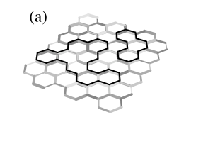
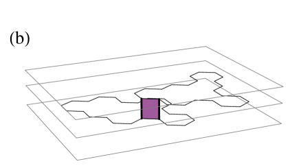
Figure 1: (a) Loops on a inhomogeneous lattice. The grayscale on each link represents the magnitude of the weight $t_{ij}$. (b) Loops on several sheets of homogeneous lattices are coupled each other. An example of a term with the first order in the coupling $t_{2}$.

Although we perform the detailed analysis in continuum theory, let us proceed, for a while, within the discrete lattice formulation. The purpose is two-fold: (i) to get some insight on underlying physics, as we can concretely see the elementary processes existing in the model and (ii) to see that there are possibly many lattice models described by the same continuum field theory. Now, we consider the $M$ copies of the model (3) and take the disorder average. This gives

$$\eqalign{\overline{\left(Z\left[\{t\},n\right]\right)^{M}}&=\int\prod_{\langle i,j\rangle}dt_{ij}P(t_{ij})\prod_{a=1}^{M}\Tr_{s^{(a)}_{i}}\ \prod_{\langle i,j\rangle}\left(1+t_{ij}s^{(a)}_{i}\cdot s^{(a)}_{j}\right)\\ &=\prod_{a=1}^{M}\Tr_{s^{(a)}_{i}}\ \prod_{\langle i,j\rangle}\left(1+t_{1}\sum_{a=1}^{M}s^{(a)}_{i}\cdot s^{(a)}_{j}+t_{2}\sum_{a<b}^{M}s^{(a)}_{i}\cdot s^{(a)}_{j}\ s^{(b)}_{i}\cdot s^{(b)}_{j}\right)\\ &\hskip 28.45274pt+\left(\mathrm{higher\ order\ terms}\right),}$$ (10)

where in the last line, the first two moments are denoted as $t_{1}=\overline{t_{ij}}$ and $t_{2}=\overline{t_{ij}^{2}}$, and we omit the terms with the higher moments for simplicity. The term $t_{1}\,\left(s^{(a)}_{i}\cdot s^{(a)}_{j}\right)$ represents a walk on the same replica layer; the generic case with $t_{1}\neq 0$ is discussed in the following. In addition to this, the theory acquires nonlinear couplings. For instance, when we look at a particular path of a loop, the coupling $t_{2}\,\left(s^{(a)}_{i}\cdot s^{(a)}_{j}\ s^{(b)}_{i}\cdot s^{(b)}_{j}\right)$ for $a<b$ is considered as a branching process across the replica direction as shown in Figure 1-(b). On a lattice, evaluating directly the contribution of the diagrams with the second or higher orders in such processes should involve some sophisticated enumerative combinatorics. Notice, however, that the translational invariance of the individual $O(n)$ model is now restored. Thus, in the continuum limit, we can use the knowledge of the homogeneous $O(n)$ CFT.

The restriction on the sum to off-diagonal sector $(a<b)$ in the $t_{2}$ term follows from the fact that the original partition function (3) is linear in the bonds $(t_{ij}\,s_{i}\cdot s_{j})$. When we talk about the universality, however, this formal linearity and resulting off-diagonal property should be reconsidered; we should rather consider a larger parameter space including more general couplings generated under block spin transformations.

In order to see this, firstly, it is instructive to remind that the pure model (1) corresponds to the Hamiltonian $H=-\sum\ln(1+ts_{i}\cdot s_{j})$, and originates from the high temperature expansion of another spin system which has the same $O(n)$ symmetry but has the different Hamiltonian $H=-\beta\sum s_{i}\cdot s_{j}$. From the RG perspective, these two models are regarded as two different points in the same theory space determined from the $O(n)$ symmetry. Actually, both systems are believed to belong to the same universality class. In fact, with the knowledge of the scaling dimensions of fields obtained by the CG method [18], we may argue that these two Hamiltonians are equivalent modulo irrelevant operators. In particular, the field $(s_{i}\cdot s_{j})^{2}$ represents the double occupancy of the bonds in the partition function, and the presence of it enables the loops to overlap. Although such a field is not contained in the partition function (1), it is natural to think that the term $(s_{i}\cdot s_{j})^{2}$ is generated, under block spin transformation, from the single occupation $(s_{i}\cdot s_{j})$. But, as we will see in the end of Section 2.2, the term $(s_{i}\cdot s_{j})^{2}$ is irrelevant in the dilute phase, or equivalently, near the critical point. Because of this, we can say that the linear expression (1) nicely summarize the characteristics of the dilute phase in generic models with the $O(n)$ symmetry.

Taking these considerations into account, we now briefly discuss the theory space of the coupled models derived from the disordered ones. Our concern is near the decoupled critical point; applying the knowledge of the pure $O(n)$ model, we note the inessential differences that arise from different formulations of disordered models on a lattice. For concreteness, let us consider another disordered model:

$$Z\left[\{\beta\},n\right]=\Tr_{s_{i}}\prod_{\langle ij\rangle}\exp\left(\beta_{ij}s_{i}\cdot s_{j}\right),$$ (11)

with a bond distribution $P(\beta)$. The formal operations lead to, again, a coupled model:

$$\eqalign{\overline{\left(Z\left[\{\beta\},n\right]\right)^{M}}&=\prod_{a=1}^{M}\Tr_{s^{(a)}_{i}}\ \prod_{\langle i,j\rangle}\exp\left(\beta_{1}\sum_{a=1}^{M}s^{(a)}_{i}\cdot s^{(a)}_{j}+\beta_{2}\sum_{a=1,\,b=1}^{M}s^{(a)}_{i}\cdot s^{(a)}_{j}\ s^{(b)}_{i}\cdot s^{(b)}_{j}\right)\\ &\hskip 28.45274pt+\left(\mathrm{higher\ order\ terms}\right),}$$ (14)

where $\beta_{1}=\overline{\beta_{ij}}$ and $\beta_{2}=\frac{1}{2}\left(\overline{\beta_{ij}^{2}}-\overline{\beta_{ij}}^{2}\right)$ are the first and the second cumulants obtained from the distribution $P(\beta_{ij})$, respectively. Comparing this model (14) with the previous one (10), we notice that the differences between these two are simply the presence of the exponential function and that of the diagonal coupling: $\beta_{2}\,\left(s^{(a)}_{i}\cdot s^{(a)}_{j}\ s^{(b)}_{i}\cdot s^{(b)}_{j}\right)$ with $a=b$ in (14). Both features lead to the term $\left(s_{i}^{(a)}\cdot s_{j}^{(a)}\right)^{2}$ i.e. the process of the double occupancy of the bonds on the same replica plane. Such a term can also be generated in the model (10) under block spin transformation. However, when the corresponding pure model is in the dilute phase, the process is irrelevant. For this reason, we expect both of the coupled models (10) and (14) are described by a same field theory.

A related model, which is more suitable for taking continuum limit, can be formulated with a probability distribution $P_{s}(\mu)$ for disorders $\mu$ on each site:

$$Z\left[\{\mu\},n\right]=\Tr_{s_{i}}\prod_{\langle ij\rangle}\exp\biggl{[}\left(\mu_{i}+\mu_{j}\right)s_{i}\cdot s_{j}\biggr{]}.$$ (15)

In this model, the bond strength $\tilde{\beta}_{ij}=\mu_{i}+\mu_{j}$ respects a distribution $\tilde{P}$ obtained by the convolution of two $P_{s}$ i.e. $P_{s}*P_{s}=\tilde{P}$. If this distribution $\tilde{P}(\tilde{\beta})$ is identical to the distribution $P(\beta)$ in (11), then this model becomes similar to that of (11). Still, the model (15) is different from the model (11), since there exists the correlation between the nearest-neighbor bonds (say $\tilde{\beta}_{ij}$ and $\tilde{\beta}_{ik}$) connected at a site. Nevertheless, the correlation is still short range; we expect a similar behavior at large scales.

We can argue that this correlation existing in the model (15) is not essential to distinguish it from the model (11) by examining how these two models are mapped into the theory space of the coupled models. Averaging over the disorder $\mu$ in (15) yields, at a site $i$, a term $\sum_{a,b,j,k}\left(s^{(a)}_{i}\cdot s^{(a)}_{j}\ s^{(b)}_{i}\cdot s^{(b)}_{k}\right)$ as a leading nonlinear coupling. In particular, the $j\neq k$ part of this coupling is induced by the correlation between the nearest-neighbor bonds in the model (15). If this coupling were, with some special reason, never generated in the model (14) mapped from (11), we would seriously distinguish (15) from (11) in the first place. But, it has already been contained in (14), implicitly. Indeed, although the expression (14) is written with respect to links, this can be recasted in terms of sites thanks to the discrete rotational and the discrete translational invariance of the coupled model on a lattice. Then we recognize, by expanding the exponential, this coupling is also present in the model (14).

To summarize, in the dilute phase, there are two important processes on a lattice: the walk on the same layer $\left(s_{i}^{(a)}\cdot s_{j}^{(a)}\right)$ and the branching to another layer $\left(s^{(a)}_{i}\cdot s^{(a)}_{j}\ s^{(b)}_{i}\cdot s^{(b)}_{j}\right)$ for $a\neq b$. It is plausible to think that these coupled models discussed here are, at large scales, described by a simple continuum field theory.

2.2 Critical point of the homogeneous $O(n)$ model

When we approach a critical point of some lattice model defined in the dimension $d$, the correlation length $\xi$ of the model, which is usually the order of the lattice cut-off $a$, becomes arbitrary large. The continuum limit (or, scaling limit) of the lattice model can be reached by taking $a\rightarrow 0$, while keeping $\xi$ fixed. There is nice class of local lattice observables $\{\phi_{k}^{\mathrm{lat}}\}$ which have the finite limit

$$\lim_{a\rightarrow 0}a^{-2(\Delta_{\phi_{1}}+\cdots+\Delta_{\phi_{n}})}\langle\phi_{1}^{\mathrm{lat}}(x_{1})\cdots\phi_{n}^{\mathrm{lat}}(x_{n})\rangle=\langle\phi_{1}(x_{1})\cdots\phi_{n}(x_{n})\rangle,$$ (16)

for an appropriate choice of scaling dimensions $\{2\Delta_{\phi_{k}}\}$. With the idea of the block spin transformation, the scaling fields $\phi_{k}(x_{k})$ may be considered as coarse grained versions of $\phi_{k}^{\mathrm{lat}}$ over some region of size $L$, centered at $x_{k}$, with $a\ll L\ll\xi$. These scaling dimensions are determined dynamically from the interactions in the system, and related to the RG eigenvalues $y_{\phi_{k}}$ via $y_{\phi_{k}}=d-2\Delta_{\phi_{k}}$. When $y_{\phi_{k}}$ is positive (negative), the RG flow near the critical point is unstable (stable), and the corresponding observable and fields are relevant (irrelevant).

Around the critical point in the theory space of the $O(n)$ model, there are, at least, two directions which are unstable (i.e. relevant) under the RG flow to the infrared. These directions are spanned by the coupling constants associated with the two most important pairs $\{\phi_{k}^{\mathrm{lat}},\phi_{k}\}$ of local lattice observables and the corresponding scaling fields. On the lattice side, one is the energy density $\sum_{j}s_{i}\cdot s_{j}$ and the other is the spin vector $s_{i}^{\alpha}$. In the scaling limit, they renormalize to become the scaling fields called the energy operator ${\cal E}(x)$ and the spin operator $\sigma(x)$. The scaling dimension of ${\cal E}(r)$ and that of $\sigma(r)$ is related to the leading thermal and the leading magnetic eigenvalue of the spin system, respectively. These two positive eigenvalues correspond to the linearized RG flow near the critical point, and determine the thermodynamic exponents [16].

	Lattice	Continuum	primary fields	scaling dimension
energy	$\sum_{j}s_{i}\cdot s_{j}$	${\cal E}(x)$	$\phi_{1,3}$	$-2+4\alpha_{-}^{2}$
spin	$s_{i}^{\alpha}$	$\sigma(x)$	$\phi_{p-1,p}$	$1-\alpha_{-}^{2}/2-3/(8\alpha_{-}^{2})$
polarization	$s_{i}\!{}^{\alpha}s_{i}\!{}^{\beta}$	$\sigma_{\rm{II}}(x)$	$\phi_{1,0}$	$1-\alpha_{-}^{2}/2$
encounter	$\sum_{j}(s_{i}\cdot s_{j})^{2}$	$\sigma_{\rm{IV}}(x)$	$\phi_{2,0}$	$1-\alpha_{-}^{2}/2+3/(2\alpha_{-}^{2})$

Table 1: Correspondence between lattice observables and continuum fields. The value of $p$ is given by $p=1/(2-2\alpha_{-}^{2})$.

So far, we have described the qualitative structure of the theory space focusing on the correspondence between the lattice observables and the continuum scaling fields. It is tantalizing that there is no versatile scheme for a given lattice model to establish this type of correspondence and to proceed to quantitative analysis using a scaling theory at hand. However, the $O(n)$ model was particularly successful in this respect; the geometric nature such as the loop representation of the partition function made it possible to access some of the exact results on the scaling dimensions by the CG method [18] before the emergence of the conformal field theory [3]. These exact results by the CG method, or by the other means [14] then led to the conjecture claiming that a certain one-parameter family of CFT’s describe the critical points of $O(n)$ model for the continuous value of $n\ (|n|\leq 2$) [12]. This claim is further checked by the Bethe ansatz result [2].

We assume this one-parameter family of CFT’s [12] in the rest of the paper. The correlation functions of primary fields are represented in terms of the vertex operators $\{e^{i\alpha_{k}\phi(x)}\}$ with an appropriate choice of charges $\{\alpha_{k}\}$, where $\phi(x)$ is a bosonic scalar field [12, 15, 33]. The necessary formulae on the vertex operator representation are given in Appendix A. In this construction, we have two marginal operators (the screening vertex operators). In the $O(n)$ model, the screening charge $\alpha_{-}$ is related to $n$ as

$$n=-2\cos\left(\pi/\alpha_{-}^{2}\right).$$ (17)

The energy operator and the spin operator is identified with the primary fields as follows:

$${\cal E}(x)\rightarrow\phi_{1,3},\qquad\sigma(x)\rightarrow\phi_{p-1,p},$$ (18)

where the value of $p$ is given by $p=1/(2-2\alpha_{-}^{2})$. These identifications are based on the dimensions originally obtained by the CG methods given in Table 1. Using the formulas (102) and (103), the dimensions of these operators are checked as

$$2\Delta_{\cal E}=-2\alpha_{1,3}\alpha_{\overline{1,3}}=-2(-\alpha_{-})(\alpha_{+}+2\alpha_{-})=-2+4\alpha_{-}^{2},$$ (19)

$$2\Delta_{\sigma} =-2\alpha_{p-1,p}\alpha_{\overline{p-1,p}}=-\frac{1}{2}\left((2-p)\alpha_{+}+(1-p)\alpha_{-}\right)\left(p\alpha_{+}+(1+p)\alpha_{-}\right)$$ (20)

$$=1-\alpha_{-}^{2}/2-3/(8\alpha_{-}^{2}).$$

where $\alpha_{+}\alpha_{-}=-1$ in (100) is used.

The relation to the two dimensional critical statistical models are summarized below. The $O(n)$ model at $n=2$ ($\alpha_{-}^{2}=1$) and $n=1$ ($\alpha_{-}^{2}=\frac{3}{4}$) are the XY model and the Ising model, respectively. The Ising model is the only minimal unitary model [3] that belongs to the $O(n)$ family. Note that the Ising model is also regarded as the $q$-state Potts model at $q=2$ [8]. The model at $n=0$ ($\alpha_{-}^{2}=\frac{2}{3}$) corresponds to the polymer, or self avoiding walk (SAW), as the qualitative result was obtained by $\epsilon=4-d$ expansion [26]. The model in two dimensions is related, under the SLE duality [32], to the percolation (Potts model at $q=1$). Both models are non-unitary, and various scaling dimensions in the models are numerically studied in ref. [28]. Finally, the model at $n=-2$ ($\alpha_{-}^{2}=\frac{1}{2}$) is the loop-erased random walk (LERW). The one-parameter family of $O(n)$ CFT’s are related to the SLE by

$$\kappa=4\alpha_{-}^{2},$$ (21)

where $\kappa$ is the strength of the Brownian motion which drives the evolution SLE. These critical $O(n)$ models covers $2\leq\kappa\leq 4$.

In the rest of the sub-section, we discuss more on the correspondence between the lattice and the continuum. The relation between the loop configuration and the correlation function in the continuum theory is given; the latter is the object of our study henceforth. The reader who is not interested in the lattice may skip the following.

In this paper, we restrict our consideration to the calculation of the RG flow in the subspace spanned by the coupling constant associated with the energy operator ${\cal E}$ and the spin operator $\sigma$. There is, however, another important RG eigenvalue apart from the ones associated with these two; the eigenvalue is responsible for the geometric property of the loops. In other words, the thermal and the magnetic eigenvalues are not sufficient to characterize the local shape of the loops even at a primitive level. To see this, let us first remind that, in the SAW ($n=0$), the fractal dimension $D_{F}$ of the loop is given by the thermal eigenvalue $y_{\cal E}$, and thus $D_{F}=1/\nu$ [26]; it is then given by $y_{\cal E}=2-2\Delta_{{\cal E}}=\frac{4}{3}$ in two dimensions. The generalization of this result to arbitrary $n$ $(|n|\leq 2)$ was discussed by relating the $O(n)$ loops to the clusters in the percolation [57]. The fractal dimension for $n\neq 0$ should then be written as

$$D_{F}=\frac{1}{\sigma_{F}\nu},$$ (22)

with $\sigma_{F}\neq 1$ (in the percolation theory, $\sigma_{F}$ is called the Fisher exponent, and $\nu$ the correlation length exponent). Further, the fractal dimension $D_{F}$ is expected to be the RG eigenvalue from the polarization operator (or, the two-leg operator): $\{\phi^{\rm lat},\phi\}=\{s_{i}^{\alpha}s_{i}^{\beta},\sigma_{\rm{II}}(x)\}$ with the vector indexes $\alpha\neq\beta$, for which the scaling dimension can be obtained by the CG method (see Table 1). The fractal dimension of the $O(n)$ loop in the dilute phase is then given by $D_{F}=2-2\Delta_{\sigma_{\rm{II}}}=1+\alpha_{-}^{2}/2$ .

Diagrammatically, the polarization operator $\sigma_{\rm{II}}(x)$, when inserted into a correlation function, creates two curves emanating from a point $x$, while the spin operator $\sigma(x)$ creates only one curve. The curves created by $\sigma_{\rm{II}}(x)$ repel each other; they have different colors $\alpha\neq\beta$ and hence can not connect by themselves. They need to be annihilated by the other operator $\sigma_{\rm{II}}(y)$. By contrast, the insertion of the energy operator ${\cal E}(x)$ require that a point $x$ be passed by some loop; the curve passing the point will connect each end to form the loop.

However, forming a loop becomes more and more difficult as $n$ tends to zero; the loop segments repel each other in the SAW. In this sense, the role of the energy operator ${\cal E}$ approaches that of the polarization operator $\sigma_{\rm{II}}$. In fact, at the SAW, these two operators has the same scaling dimension $2\Delta=\frac{2}{3}$, and this explain $\sigma_{F}=1$ in (22). In the CFT context, by using the scaling dimensions obtained by the CG method, $\sigma_{\rm{II}}(x)$ was argued to correspond to the $\phi_{1,0}$ primary field. Then, $\sigma_{F}=1$ can be confirmed by the well-known equivalence between the primary field:

$$\phi_{r,s}=\phi_{m-r,m+1-s}\qquad(0\leq r\leq m,\,0\leq s\leq m+1),$$ (23)

in the $m$-th minimal model with the central charge $c=1-6/m(m+1)$. Indeed, in the SAW, which is the $m=2$ minimal model, $\phi_{1,3}$ (the energy operator ${\cal E}$) should have the same dimension as the field $\phi_{1,0}$ (the polarization operator $\sigma_{\rm{II}}$), since $(1,3)+(1,0)=(2,3)$.

There are, of course, many other composite fields constructed as products of the several local lattice observables. A quantitative discussion on such fields is given, which is based on the OPE and the correlation inequalities [19]. Their result suggests, in general situation, that the scaling dimension of a composite field exceeds the sum of those of the elementary fields due to the repulsion between them. This implies higher-order composite fields are more likely to be irrelevant in the RG. In our context, we mention the four-leg operator $\{\sum_{j}(s_{i}\cdot s_{j})^{2},\sigma_{\rm{VI}}(x)\}$ as an important example [18, 33]. The insertion of the field $\sigma_{\rm{VI}}(x)$ into a correlation function corresponds to requiring two of the loop segments to overlap; in the particle picture, the trajectories should encounter at the point $x$. Again, the dimension of the field $\sigma_{\rm{VI}}(x)$ is obtained by the CG method, and identified with the primary field $\phi_{2,0}$ in the CFT. Now, we see that it is relevant in the dense phase ($\kappa>4$) and irrelevant in the dilute phase ($\kappa<4$) as shown in Fig 2. As used in Section 2.1, the latter observation is a key ingredient in understanding the universality of the pure $O(n)$ model in the dilute phase. Further, at the level of coupled model, this is crucial in our expectation that (10) and (14) are, near the decoupled critical points, described by a same field theory.

2.3 Scaling limit of the disordered $O(n)$ models

We shall go into the continuum formulation of the disordered models by using the CFT description of the critical $O(n)$ model. In section 2.1, we have considered, on the lattice, three disordered models whose partition functions are given by (3), (11) and (15). As we have seen, after the disorder averaging, they have much in common when mapped to the coupled models. When the couplings between replicas are sufficiently small, one could, by looking at (10) for instance, guess the action of the coupled models in the continuum limit. But we shall take the other way. Instead, we first consider the continuum limit of the disordered model (15), and then take the disorder average in the continuum theory. The advantage is that we can use the OPE to deal with the composite operators.

In the following, we will use the relation:

$$\prod_{\langle i,j\rangle}(1+ts_{i}\cdot s_{j})\sim\exp\left[\beta\sum_{\langle i,j\rangle}s_{i}\cdot s_{j}\right]\rightarrow\exp\left[-S_{*}+m\int d^{2}x\ {\cal E}(x)\right].$$ (24)

The first equivalence symbol means that these two pure model belong to the same universality class, as discussed in the paragraph above (11). In the right hand side, we formally write the action of the $O(n)$ CFT as $S_{*}$. The coupling constant $m$ is proportional to the reduced temperature, which is given by $(t-t_{c})/t_{c}$, or $(\beta-\beta_{c})/\beta_{c}$.

Using the relation (24), it is natural to assume the continuum limit of the model (15) is described by

$$\left(Z\left[\{\mu\},n\right]\right)^{M}=\int\prod_{a=1}^{M}\mathcal{D}\Phi^{(a)}(x)\ \exp\left[-\left(\sum_{a=1}^{M}S_{*}^{(a)}\right)+\int d^{2}x\ m(x)\left(\sum_{a=1}^{M}{\cal E}^{(a)}(x)\right)\right],$$ (25)

where $S_{*}^{(a)}$ is the action of the $O(n)$ CFT on the replica plane $(a)$. Here, we formally write elementary fields (in the sense of [7]) as $\Phi^{(a)}(x)$ and replace the tracing $\Tr_{s^{(a)}_{i}}$ in (15) to $\int\mathcal{D}\Phi^{a}(x)$, which denotes the path integration over the fluctuation of $\Phi^{(a)}(x)$. The realization $\{\mu\}$ of the local weights $\mu_{i}$ on lattice sites in (15) are now replaced to its continuum counterpart, that is, a configuration of a scalar function $m(x)$. Physically, this $m(x)$ serves as a locally fluctuating reduced temperature. We assume this $m(x)$ respects a single distribution function $\hat{P}\left(m(x)\right)$ which is independent of the position $x$. Hereafter, we suppress the argument of the partition function $Z\left[\{\mu\},n\right]$. Then the averaging operation is written as

$$\overline{Z^{M}}=\int\mathcal{D}m(x)\hat{P}\left(m(x)\right)\ Z^{M},$$ (26)

where $\mathcal{D}m(x)$ denotes a path integral measure $\prod_{x}dm(x)$. Let $\hat{\xi}_{k}$ be a $k$-th cumulant of the distribution function $\hat{P}(m(x))$. In the important case of a Gaussian distribution $\hat{P}(m(x))=\exp\left[-(m(x)-\hat{m}_{0})^{2}/2\hat{g}_{0}\right]$, we have $\hat{\xi}_{1}=\hat{m}_{0}$, $\hat{\xi}_{2}=\hat{g}_{0}$ and $\hat{\xi}_{k}=0$ for $k\geq 3$. Then, by the averaging over the disorder, we obtain

$$\overline{Z^{M}} =\int\prod_{a=1}^{M}\mathcal{D}\Phi^{a}(x)\ \exp\left[-\sum_{a=1}^{M}S_{*}^{(a)}+\int d^{2}x\ \left(\hat{\xi}_{1}\sum_{a=1}^{M}{\cal E}^{(a)}(x)+\hat{S}_{I}(x)\right)\right],$$ (27)

$$\hat{S}_{I}(x) =\hat{\xi}_{2}\sum_{a,b}^{M}{\cal E}^{(a)}(x){\cal E}^{(b)}(x)+\hat{\xi}_{3}\sum_{a,b,c}^{M}{\cal E}^{(a)}(x){\cal E}^{(b)}(x){\cal E}^{(c)}(x)+\cdots.$$ (28)

In this formal expression, we should note that the nonlinear part $\hat{S}_{I}(x)$ contains the composite operators i.e. the products of the several fields at the same point on the same replica plane. We deal with them by using the fusion rules in the $O(n)$ model. According to the identification ${\cal E}\rightarrow\phi_{1,3}$ in (18), the fusion rule in the thermal sector reads

$$\phi_{1,3}\cdot\phi_{1,3}\sim\phi_{1,1}+\phi_{1,3}+\phi_{1,5},$$ (29)

or, equivalently,

$${\cal E}\cdot{\cal E}\sim I+{\cal E}+{\cal E}^{\prime}.$$ (30)

Here, ${\cal E}^{\prime}=\phi_{15}$ is the next-leading energy operator.

Figure 2: The scaling dimensions $2\Delta$ of the primary fields $\phi_{1,3}$, $\phi_{1,5}$ and $\phi_{2,0}$ plotted as functions of the SLE parameter $\kappa=4\alpha_{-}$. The horizontal line at $2\Delta=1$ shows the marginality of the most relevant couping ${\cal E}^{(a)}(x){\cal E}^{(b)}(x)$.

Since this operator is irrelevant as shown in Figure 2, we neglect the ${\cal E}\cdot{\cal E}\rightarrow{\cal E}^{\prime}$ part of the OPE (30). The identity field $I=\phi_{11}$ contributes as a trivial shift of the free energy. The emergence of the energy operator ${\cal E}$ in the right hand side of (30) is a characteristic of $O(n)$ model with $n\neq 1$, which will be discussed in the paragraph below (39). Because of this contribution (${\cal E}\cdot{\cal E}\rightarrow{\cal E}$), qualitatively speaking, we should have a hierarchical flow of the coupling constants: $\cdots\rightarrow\hat{\xi}_{3}\rightarrow\hat{\xi}_{2}\rightarrow\hat{\xi}_{1}$. For example, the diagonal ($a=b$) part of $\hat{\xi}_{2}\sum{\cal E}^{(a)}(x){\cal E}^{(b)}(x)$ mixes with $\hat{\xi}_{1}\sum{\cal E}^{(a)}$ and hence the flow $\hat{\xi}_{2}\rightarrow\hat{\xi}_{1}$ occurs . Thus, by redefining the coupling constants $\hat{\xi}_{k}$ , we get

$$\overline{Z^{M}} =\int\prod_{a=1}^{M}\mathcal{D}\Phi^{a}(x)\ \exp\left[-\sum_{a=1}^{M}S_{*}^{(a)}+\int d^{2}x\ \left(m_{0}\sum_{a=1}^{M}{\cal E}^{(a)}(x)+S_{I}(x)\right)\right],$$ (31)

$$S_{I}(x) =g_{0}\sum_{a\neq b}^{M}{\cal E}^{(a)}(x){\cal E}^{(b)}(x)+\xi_{3}\sum_{a\neq b,b\neq c,c\neq a}^{M}{\cal E}^{(a)}(x){\cal E}^{(b)}(x){\cal E}^{(c)}(x)+\cdots,$$ (32)

where we use the symbol $m_{0}$, $g_{0}$ and $\xi_{k}$ ($k\geq 3$) for the new coupling constants. Now, the effective interaction $S_{I}(x)$ is defined without composite operators. It should be noted that we restrict our considerations on the theory space which is replica symmetric; we assume that the coupling constant for, say ${\cal E}^{(a)}(x){\cal E}^{(b)}(x)$, is independent of the pair $(a,b)$.

These coupling constants are determined by the distribution function $\hat{P}(m(x))$ in (26), and are non-zero in general. The massless limit ($m_{0}\rightarrow 0$) of the decoupled model ($g_{0}=0,\xi_{k}=0$) remains obviously as a fixed point. We now change the distribution function $\hat{P}(m(x))$, and gradually turn on the effective interaction $S_{I}$ in (32) while keeping $m_{0}=0$. The large scale behavior is then dominated by the most relevant field: ${\cal E}^{(a)}(x){\cal E}^{(b)}(x)$. The dimension of this operator is given by $4\Delta_{{\cal E}}$, which is the twice the dimension of the energy operator.

As we can infer from (19), this field becomes marginal at $n=1$ ($\alpha_{-}^{2}=\frac{3}{4}$). Since $O(1)$ model is the Ising model, this serves as a simple check of the known marginality of the disorder in the random-bond Ising model [8, 30]. Hence, we use the parametrization:

$$\alpha_{-}^{2}=\frac{3}{4}-\epsilon,$$ (33)

to perform the epsilon expansion in the next section.

3 Renormalization group flow in the one-loop calculation

In this section, we discuss the scale dependence of the theory (32) by one-loop RG calculation. It will turn out that under certain circumstances, the disordered $O(n)$ model has a pair of the ultraviolet (UV) and the infrared (IR) fixed points, as in the random-bond $q$-state Potts model [8, 20]. We will investigate the properties of the IR fixed point by which the large scale behavior of the theory is dominated.

3.1 The epsilon expansion and procedure of RG

We shall calculate the RG flow of the coupled model (32) perturbatively in the epsilon expansion using the parameter in (33). Generally, a flow is determined only by the most fundamental properties of a theory such as the symmetries and the dimension of the space. In order to grasp the topology of a theory space, it is often useful to think that these symmetries are dependent on some continuous parameters [7, 8, 20, 24], or that the dimension itself is a continuous parameter [25]. Although the change is gradual when we look locally at a generic point as varying these parameters, the global structure of the flow, on the other hand, may change drastically at certain critical values of the parameters. A typical topological transition is caused by a branching of one merged fixed point into a pair of the UV fixed point and the IR fixed point. The idea of epsilon expansion provides us with a firm ground to perform a perturbation calculation in the non-trivial region after the branching.

In the parameter space, we can infer the location of the branching by the presence of a marginal field: the hallmark of the merged fixed points. In the renowned example of the $\mathbb{Z}_{2}$-invariant scalar field theory [25], the most relevant interaction $\phi^{4}$ becomes marginal at the dimension $d=4$. In $d=4-\epsilon$, the Gaussian fixed point and the Wilson-Fisher fixed point emerge; we can do a solid perturbative calculation by setting an appropriate coupling coordinate in which the coupling constant remains $\mathcal{O}(\epsilon)$.

In the disordered $O(n)$ model, as mentioned in the previous section, the most relevant part of the effective interaction $S_{I}$ in (32) is the term ${\cal E}^{(a)}(x){\cal E}^{(b)}(x)$, which is marginal at $n=1$ and is relevant for $n<1$ (see Fig. 2). The next-leading relevant term ${\cal E}^{(a)}(x){\cal E}^{(b)}(x){\cal E}^{(c)}(x)$ is irrelevant for $n>0$ and is marginal at $n=0$ (SAW). We restrict our analysis on $n>0$, keep the most relevant part

$$S_{I}=g_{0}\sum_{a\neq b}^{M}{\cal E}^{(a)}(x){\cal E}^{(b)}(x),$$ (34)

and discard the other higher-order terms in (32).

The implementation of the RG is as follows. We introduce a cut-off length scale $r$, which serves as an effective lattice spacing, and determine a renormalized coupling $g(r)$ by integrating out the short-distance degrees of freedom:

$$\eqalign{r^{-8\epsilon}g(r)\langle S_{I}(x)S_{I}(\infty)\rangle_{0}=&g_{0}\langle S_{I}(x)S_{I}(\infty)\rangle_{0}+\frac{g_{0}^{2}}{2!}\int_{|y-x|<r}d^{2}y\langle S_{I}(x)S_{I}(y)S_{I}(\infty)\rangle_{0}\\ &+\frac{g_{0}^{3}}{3!}\int_{|y-x|<r,|z-x|<r}d^{2}yd^{2}z\langle S_{I}(x)S_{I}(y)S_{I}(z)S_{I}(\infty)\rangle_{0}+\cdots,}$$

where the insertions of the interaction fields $S_{I}$ are restricted onto a disk of radius $r$, and the coupling is measured by projecting perturbative contributions on $S_{I}(\infty)$. The symbol $\langle...\rangle_{0}$ represents the unperturbed correlation function. A trivial scaling factor $r^{-8\epsilon}$ is introduced in order to make the renormalized coupling dimensionless. At this stage in RG, as is well known, a finite redefinition of the coupling is possible; physical quantities (scaling dimensions, for instance) is invariant under a finite coordinate reparametrization of theory space [24]. To fix this ambiguity, we choose a minimal subtraction scheme. Then we get the renormalized coupling in the form:

$$g(r)=r^{8\epsilon}\left(g_{0}+G_{2}(\epsilon,r)g_{0}^{2}+G_{3}(\epsilon,r)g_{0}^{3}+\cdots\right),$$ (35)

where $G_{2}(\epsilon,r)$ and $G_{3}(\epsilon,r)$ have only poles in $\epsilon$ and no regular part . The beta function is then obtained by differentiating the renormalized coupling (35) with respect to $(\ln r)$. Using the first two terms in the fusion rule (30), we make contractions and list, in Figure 3, the possible diagrams for the beta function.

3.2 One-loop beta function, a line of random fixed points and a strong coupling region

We here calculate one-loop beta function. The process represented by the diagram in Figure 3-(a) involves three layers, and the number of the ways for this contraction is $4(M-2)$. Then we have

$$G_{2,1}(r,\epsilon) =\frac{1}{2!}\cdot 4(M-2)\int_{|y-x|<r}d^{2}y\langle{\cal E}(x){\cal E}(y)\rangle_{0}$$ (36)

$$=4\pi(M-2)\left(\frac{r^{8\epsilon}}{8\epsilon}\right),$$

where we have used $\langle{\cal E}(x){\cal E}(y)\rangle=|x-y|^{-4\Delta_{\cal E}}$ and $4\Delta_{\cal E}=2-8\epsilon$.

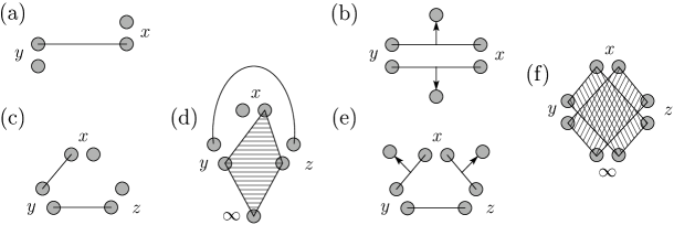
Figure 3: The diagrams for the beta function. A gray disk and a nearby pair of the disks represent an energy operator $\sum_{a}{\cal E}^{(a)}$ and the interaction $S_{I}=\sum_{a\neq b}{\cal E}^{(a)}{\cal E}^{(b)}$, respectively. An arrow corresponds to the sub-leading part of the OPE in (38) and a shaded-square represents four-point function. The external lines to the point infinity in (3.1) are amputated. The second order: (a) $G_{2,1}(r,\epsilon)$ and (b) $G_{2,2}(r,\epsilon)$; the third order: (c) $G_{3,1}(r,\epsilon)$, (d) $G_{3,2}(r,\epsilon)$, (e) $G_{3,3}(r,\epsilon)$ and (f) $G_{3,4}(r,\epsilon)$.

Besides this, up to one-loop order, there is the other contribution represented by Figure 3-(b) which is obtained by using twice the sub-leading part of the OPE (${\cal E}\cdot{\cal E}\rightarrow{\cal E}$):

$$G_{2,2}(r,\epsilon) =\frac{1}{2!}\cdot 2\int_{|y-x|<r}d^{2}y\left(\frac{C^{{\cal E}}_{{\cal E}{\cal E}}(\alpha_{-}^{2})}{|x-y|^{1-4\epsilon}}\right)^{2}$$ (37)

$$=2\pi\left[C^{{\cal E}}_{{\cal E}{\cal E}}(\alpha_{-}^{2})\right]^{2}\left(\frac{r^{8\epsilon}}{8\epsilon}\right).$$

Here, $C^{{\cal E}}_{{\cal E}{\cal E}}(\alpha_{-}^{2})$ is the structure constant of the CFT which appear in the OPE:

$${\cal E}(0,0)\cdot{\cal E}(z,\bar{z})=\frac{C_{{\cal E}{\cal E}}^{I}}{(z\bar{z})^{2\Delta_{\cal E}}}I+\frac{C_{{\cal E}{\cal E}}^{{\cal E}}}{(z\bar{z})^{\Delta_{\cal E}}}{\cal E}+\frac{C_{{\cal E}{\cal E}}^{{\cal E}^{\prime}}}{(z\bar{z})^{2\Delta_{\cal E}-\Delta_{\cal E}^{\prime}}}{\cal E}^{\prime}+\cdots,$$ (38)

where we write just the primary operators to represent their conformal families including the descendants. The structure constants are, in general, determined by the requirement that the operator algebra be associative. In practice, the crossing symmetry of the four-point function is strong enough to fix them [3]; the actual values are obtained by using either the connection matrix of the hypergeometric function [11], or the vertex operator representation of the four-point function [13]. This reads,

$$C^{{\cal E}}_{{\cal E}{\cal E}}(\rho)=2(1-2\rho)^{2}\frac{\gamma^{\frac{3}{2}}(\rho)}{\gamma^{2}(2\rho)}\frac{\gamma^{\frac{1}{2}}(2-3\rho)}{\gamma(3-4\rho)},$$ (39)

where we have used temporary notation $\rho=\alpha_{-}^{2}$ and $\gamma(x)=\Gamma(x)/\Gamma(1-x)$.

The structure constant $C^{{\cal E}}_{{\cal E}{\cal E}}(\alpha_{-}^{2})$ has information about the important selection rules in the pure $O(n)$ model. First, observe that the square of the structure constant (39) has a zero at $\alpha_{-}^{2}=\frac{3}{4}$ (the Ising model, $\epsilon=0$) and a pole at $\alpha_{-}^{2}=\frac{2}{3}$ (SAW, $\epsilon=\frac{1}{12}$). The former zero is due to the self-duality of the Ising model [17]. In the vicinity of the critical point, the duality transformation changes the sign of the reduced temperature $t$. Since the energy operator ${\cal E}$ couples to $t$, if the model is invariant under the duality, it should be odd under the duality. Then ${\cal E}$ is not allowed to appear in the right hand side of the fusion rule (30).

The pole at $\alpha_{-}^{2}=\frac{2}{3}$ emerges because of the strong repulsion between the loop segments in the limit $n\rightarrow 0$. Since the normalization of operators are fixed such that $C_{{\cal E}{\cal E}}^{I}=1$, what really happens is the divergence of the ratio $C_{{\cal E}{\cal E}}^{{\cal E}}/C_{{\cal E}{\cal E}}^{I}$. When the two loop segments approach, they will either (i) form a complete loop (to contribute the free energy) or (ii) form together a joined loop segment. Since, in the limit $n\rightarrow 0$ the process (i) is strongly suppressed by the repulsion between the loop segments, the ratio, indeed, diverges.

Taking these interpretations into the account, more intuitive representations of the second-order contributions are possible. The term $G_{2,1}(r,\epsilon)$ is represented by the diagram in which two open segments lie on two layers and one closed loop on another layer (Figure 4-(a)), while the term $G_{2,2}(r,\epsilon)$ is represented by the diagram in which two open segments lie on two layers (Figure 4-(b)).

Figure 4: The second order diagrams; see also Figure 3. (a) $G_{2,1}(r,\epsilon)$: the three-layer process with a closed loop   (b) $G_{2,2}(r,\epsilon)$: the two-layer process.

Now we sum up (36) and (37) to get

$$g(r)=r^{8\epsilon}\left\{g_{0}+2\pi\left[2(M-2)+\left[C^{{\cal E}}_{{\cal E}{\cal E}}(\alpha_{-}^{2})\right]^{2}\right]\left(\frac{r^{8\epsilon}}{8\epsilon}\right)g_{0}^{2}+\mathcal{O}(g_{0}^{3})\right\}.$$ (40)

By introducing $\tilde{g}=r^{8\epsilon}g_{0}$, we solve (40) with respect to $\tilde{g}$:

$$\tilde{g}=g(r)-\frac{2\pi}{8\epsilon}\left[2(M-2)+\left[C^{{\cal E}}_{{\cal E}{\cal E}}(\alpha_{-}^{2})\right]^{2}\right]g(r)^{2}+\mathcal{O}\left(g(r)^{3}\right).$$ (41)

Using this, the beta function up to one-loop order is then obtained as

$$\beta(g)=\frac{dg(r)}{d\ln(r)}=8\epsilon g(r)+2\pi\left\{2(M-2)+\left[C^{{\cal E}}_{{\cal E}{\cal E}}(\alpha_{-}^{2})\right]^{2}\right\}g(r)^{2}+\mathcal{O}(g(r)^{3}).$$ (42)

This beta function of the coupled model permits an IR fixed point when the coefficient of $g(r)^{2}$ is negative. As we take the limit $M\rightarrow 0$ for the disordered model, there are a competition between the terms from $G_{2,1}(r,\epsilon)$ and $G_{2,2}(r,\epsilon)$. As a result, we get two distinct regions for $0<n<1$: in the first case we have a monotonic increasing beta function; the theory goes to the strong coupling. In the second case we have an IR fixed point. The one-loop beta function suggests that the IR fixed point vanishes at $\epsilon=\frac{1}{12}\cdot 0.770861\cdots$, which corresponds to $n=n_{*}=0.26168\cdots$. The flow of the coupling constant is schematically shown in Fig. 5. It should be noted, however, that the divergence of the coupling $g$ at $n=n_{*}$ is an artifact of the one-loop calculation; if there is a positive $g^{3}$ term, the line of the IR fixed point terminates at $(n_{c},g_{c})=(n^{\prime}_{*}\,,g_{c*}^{\prime})$ with a finite coupling $g_{c*}^{\prime}$.

The strong coupling phase of the disordered model ($M\rightarrow 0$) near $n\approx 0$ is formed by the dominance of the two-layer process $G_{2,2}(r,\epsilon)$ over the three-layer process with a closed loop $G_{2,1}(r,\epsilon)$. The qualitative behavior of the absolute ratio $\mathcal{R}(n)=|G_{2,2}/G_{2,1}|$ is independent of $M$ except a special case with $M=2$, where the three-layer process is prohibited. Diagrammatically, a large $\mathcal{R}(n)$ implies that the ratio of (the number of inter-layer hopping) to (the average number of complete loops per layer) is also large. Near $n\approx 0$ region, the particles, which are destined to form a whole connected diagram, favor to sew layers together rather than to stay on one layer and to walk around avoiding their traces.

Figure 5: A schematic flow diagram of the couping constant $g$ with respect to $n$ of the disordered $O(n)$ model suggested by the one-loop beta function (42). The bold curve represents the positions of the IR fixed points.

We shall henceforth proceed to the two loop calculation to investigate the IR fixed points in the region near $n=1$ ($\epsilon\ll\frac{1}{12}$), where regarding the structure constant $C_{{\cal E}{\cal E}}^{{\cal E}}$ in (39) as $\mathcal{O}(\epsilon)$ is justifiable. In this region, the calculation turns out to be parallel to that in the study of the random-bond Potts model by Dotsenko, Picco and Pujol [20]. At one-loop level, $C_{{\cal E}{\cal E}}^{{\cal E}}=\mathcal{O}(\epsilon)$ implies $G_{2,2}=\mathcal{O}(\epsilon)$; in the minimal subtraction scheme, we drop this term. The beta function is then

$$\beta(g)=\frac{dg}{d\ln(r)}=8\epsilon g+4\pi(M-2)g^{2}+\mathcal{O}(g^{3}).$$ (43)

We left the two loop calculation of the intermediate region where $C_{{\cal E},{\cal E}}^{{\cal E}}\approx 1$ as a future problem.

4 The scaling dimensions up to the two-loop calculation

4.1 The beta function at two-loop

There are four types of third order diagrams for the beta function as listed in Figure 3-(c), (d), (e) and (f). As the diagram $G_{3,3}(r,\epsilon)$ in Figure 3-(e) have extra $\epsilon^{2}$ factor from the structure constants and the diagram $G_{3,4}(r,\epsilon)$ in Figure 3-(f) has no pole in $\epsilon$, we omit these terms in the following. The $G_{3,1}(r,\epsilon)$ in Figure 3-(c) can be calculated as

$$G_{3,1}(r,\epsilon) =\frac{1}{3!}\cdot 12(M-2)(M-3)\int_{|y-x|<r,|z-x|<r}d^{2}yd^{2}z\langle{\cal E}(x){\cal E}(y)\rangle_{0}\langle{\cal E}(y){\cal E}(z)\rangle_{0}$$ (44)

$$=8\pi(M-2)(M-3)\int_{|y|<r}dy\ y^{-1+16\epsilon}\int_{|z|<\frac{r}{|y|}}d^{2}z|z|^{-2+8\epsilon}|z-1|^{-2+8\epsilon}$$

$$=16\pi^{2}(M-2)(M-3)\frac{r^{16\epsilon}}{(8\epsilon)^{2}}+\mathcal{O}(\epsilon^{0}),$$

where we have used the asymptotic behavior of the integral for $1\ll R$:

$$\int_{|z|<R}d^{2}z|z|^{-2+8\epsilon}|z-1|^{-2+8\epsilon}=4\pi\frac{1}{8\epsilon}+\mathcal{O}(R^{-2+16\epsilon}).$$ (45)

It should be emphasized that we get no simple pole in (44).

Next, we have $G_{3,2}(r,\epsilon)$ in Figure 3-(d) containing four-point functions:

$$G_{3,2}(r,\epsilon) =\frac{1}{3!}\cdot 24(M-2)\int_{|y-x|<r,|z-x|<r}d^{2}yd^{2}z~{}\langle{\cal E}(x){\cal E}(y){\cal E}(z){\cal E}(\infty)\rangle_{0}\langle{\cal E}(y){\cal E}(z)\rangle_{0}$$ (46)

$$=8\pi(M-2)\int_{y<r}dy\ y^{-1+16\epsilon}\,\mathcal{I}\left(r/|y|,\epsilon\right),$$ (47)

where we define

$$\mathcal{I}(R,\epsilon)=\int_{|z|<R}d^{2}z\langle{\cal E}(0){\cal E}(1){\cal E}(z){\cal E}(\infty)\rangle_{0}\langle{\cal E}(1){\cal E}(z)\rangle_{0}.$$ (48)

Actually, instead of $\mathcal{I}(R,\epsilon)$, we shall calculate $\mathcal{I}(\infty,\epsilon)$ by analytic continuation in B, and see that $\mathcal{I}(\infty,\epsilon)$ itself has no poles in $\epsilon$. Although, in the Appendix, we prove this fact by applying the contiguity relation between generalized hypergeometric series, the fact can also be interpreted as a result of a cancellation between two poles with opposite sign, as explained in the following .

In the limit $|z|\rightarrow\infty$, the integrand in (48) behaves as $|z|^{-4\Delta_{\cal E}}$ ($4\Delta_{\cal E}=2-8\epsilon$), since the four-point function, using the identity operator $I$ in (38) as the leading intermediate channel, decouples into two two-point functions. Hence, $\mathcal{I}(\infty,\epsilon)$ has the contributions from both regions $|z|<R$ and $|z|>R$, each of which contains a pole $+2\pi R^{8\epsilon}/8\epsilon$ and $-2\pi R^{8\epsilon}/8\epsilon$, respectively; they are canceled out each other. Observing that $\mathcal{I}(R,\epsilon)$ does not have the latter pole, and estimating the corrections, we obtain

$$\mathcal{I}(R,\epsilon)=2\pi\frac{R^{8\epsilon}}{8\epsilon}+\mathcal{I}(\infty,\epsilon)+\mathcal{O}(R^{-1+8\epsilon}).$$ (49)

As the first term corresponds to the decoupling limit $y\rightarrow x$ of the four-point function in (46), it leads to the same contribution as (44), only if we replace $(M-2)$ in (47) by $(M-2)(M-3)$. Now, using the vertex operator representation, we write $\mathcal{I}(\infty,\epsilon)$ in (49) as

$$\mathcal{I}(\infty,\epsilon) =\mathcal{N}\int d^{2}zd^{2}ud^{2}v\, \langle V_{\alpha_{13}}(0)V_{\alpha_{13}}(1)V_{\overline{\alpha_{13}}}(z)V_{\alpha_{13}}(\infty)V_{\alpha_{-}}(u)V_{\alpha_{-}}(v)\rangle\langle V_{\alpha_{13}}(1)V_{\overline{\alpha_{13}}}(z)\rangle$$ (50)

$$=\mathcal{N}\int d^{2}zd^{2}ud^{2}v\, |z|^{4\alpha_{13}\overline{\alpha_{13}}}|1-z|^{8\alpha_{13}\overline{\alpha_{13}}}|(z-u)(z-v)|^{4\overline{\alpha_{13}}\alpha_{-}}$$

$$\cdot|uv(u-1)(v-1)|^{4\alpha_{13}\alpha_{-}}|u-v|^{4\alpha_{-}^{2}},$$

where $\mathcal{N}$ is the normalization factor with the four-point function given in (104). Substituting (49) and the result (181) for $\mathcal{I}(\infty,\epsilon)$ into (47), we obtain

$$G_{3,2}(r,\epsilon) =16\pi^{2}(M-2)\left[\frac{1}{(8\epsilon)^{2}}-\frac{1}{8\epsilon}\right]r^{16\epsilon}+\mathcal{O}(\epsilon^{0}).$$ (51)

We get, by collecting the third order terms (44) and (51), the renormalized coupling constant in (35) as

$$g(r)=r^{8\epsilon}\left\{g_{0}+4\pi\frac{(M-2)}{8\epsilon}r^{8\epsilon}g_{0}^{2}+16\pi^{2}\left[\frac{(M-2)^{2}}{(8\epsilon)^{2}}-\frac{(M-2)}{8\epsilon}\right]r^{16\epsilon}g_{0}^{3}\right\}+\mathcal{O}(g_{0}^{4}).$$ (52)

Then (52) is solved with respect to $\tilde{g}=r^{8\epsilon}g_{0}$ as

$$\tilde{g}=g(r)-4\pi\frac{(M-2)}{8\epsilon}g(r)^{2}+16\pi^{2}\left[\frac{(M-2)^{2}}{(8\epsilon)^{2}}+\frac{(M-2)}{8\epsilon}\right]g(r)^{3}.$$ (53)

Consequently, we obtain the RG beta function

$$\beta(g)=\frac{dg(r)}{d\ln r}=8\epsilon g+4\pi(M-2)g^{2}-16\pi^{2}(M-2)g^{3}+\mathcal{O}(g^{4}).$$ (54)

As is expected from the known equivalence of the random-bond Ising model to the random-mass fermion model and the Gross-Neveu model [30, 8], at the Ising point $\epsilon=0$ ($n=1$), the expression (54) reduces to the two-loop beta function for the Gross-Neveu model [34]. Solving $\beta(g_{c})=0$ for the disordered model ($M\rightarrow 0$), we obtain the coupling constant at the random fixed point as

$$g_{c}=\frac{\epsilon}{\pi}+\frac{4\epsilon^{2}}{\pi}+\mathcal{O}(\epsilon^{3}).$$ (55)

4.2 The correction to the scaling dimensions

In our perturbation theory, the two-point correlation function between fields $\mathcal{O}(0)$ and $\mathcal{O}(\infty)$ is calculated as

$$\eqalign{\langle\mathcal{O}(0)\mathcal{O}(\infty)\rangle=\langle\mathcal{O}(0)\mathcal{O}(\infty)\rangle_{0}&+g_{0}\int_{|y|<r}d^{2}x\,\langle S_{I}(y)\mathcal{O}(0)\mathcal{O}(\infty)\rangle_{0}\\ &+\frac{g_{0}^{2}}{2!}\int_{|y|<r,~{}|z|<r}d^{2}y\,d^{2}z\,\langle S_{I}(y)S_{I}(z)\mathcal{O}(0)\mathcal{O}(\infty)\rangle_{0}+\cdots}.$$ (56)

Again, as in (3.1), we restrict the insertion of the interaction $S_{I}$ around the field $\mathcal{O}(0)$ within the disk of radius $r$. From this, we can determine a renormalization constant $Z_{\mathcal{O}}$ for the field $\mathcal{O}$ perturbatively as

$$\langle\mathcal{O}(0)\mathcal{O}(\infty)\rangle=Z_{\mathcal{O}}\langle\mathcal{O}(0)\mathcal{O}(\infty)\rangle_{0}.$$ (57)

The two-point functions in the theories with different cut-offs $r$ and $sr$ are related as

$$\langle\mathcal{O}(0)\mathcal{O}(sR)\rangle_{sr,g(sr)} =\frac{Z_{\mathcal{O}}^{2}(g(sr))}{Z_{\mathcal{O}}^{2}(g(r))}s^{-4\Delta_{\mathcal{O}}}\langle\mathcal{O}(0)\mathcal{O}(R)\rangle_{r,g(r)}$$ (58)

$$=\exp\left[2\int_{g(r)}^{g(sr)}dg~{}\frac{\gamma_{\mathcal{O}}(g)}{\beta(g)}\right]s^{-4\Delta_{\mathcal{O}}}\langle\mathcal{O}(0)\mathcal{O}(R)\rangle_{r,g(r)},$$

where, in the second line, we have introduced the anomalous dimension

$$\gamma_{\mathcal{O}}(g)=\frac{\mathrm{d}Z_{\mathcal{O}}(g)}{\mathrm{d}\ln r}.$$ (59)

Now consider the large $s$ behavior of (58) and let the upper limit $g(rs)$ of the integral tend to $g_{c}$ of the random fixed point; the beta function $\beta(g)$ tends to zero, while the anomalous dimensions $\gamma_{\mathcal{O}}(g)$, as we will see, remain finite both for the energy operator ${\cal E}$ and the spin operator $\sigma$. This means the integral is dominated by the contribution from the region $g\approx g_{c}$, and we obtain

$$2\left(\Delta_{\mathcal{O}}^{\mathrm{IR}}-\Delta_{\mathcal{O}}^{\mathrm{UV}}\right)=-\gamma_{\mathcal{O}}(g_{c}),$$ (60)

where we mean, by $2\Delta_{\mathcal{O}}^{\mathrm{IR}}$ and $2\Delta_{\mathcal{O}}^{\mathrm{UV}}$, the scaling dimension of the field $\mathcal{O}$ at the IR (the random) fixed point and the UV fixed point, respectively.

Figure 6: The contributions for the scaling dimensions. The diagrams (a), (b) (c) and (d) are for $Z_{\cal E}$, while (e) $\mathcal{S}_{2}(r,\epsilon)$ and (f) $\mathcal{S}_{3}(r,\epsilon)$ are for $Z_{\sigma}$. The white circle represents the spin operator $\sigma^{(a)}$; for symbols, see also the caption in Figure 3.

4.3 Scaling dimension of the energy operator

The first and second order diagrams for the renormalization constant of the energy operator $Z_{\cal E}$ are listed in Figure 6-(a), (b), (c) and (d). As the integral in the diagram in Figure 6-(c) does not have pole in $\epsilon$, we omit this term from the calculation. Since the integrals are same as those for the two loop beta function, by adapting combinatorial factors, we have

$$Z_{\cal E} =1+g_{0}\cdot\frac{2(M-1)}{2(M-2)}G_{2,1}+\frac{g_{0}^{2}}{2!}\left[\frac{8(M-1)(M-2)}{2(M-2)(M-3)}G_{3,1}+\frac{4(M-1)}{4(M-2)}G_{3,2}\right]$$ (61)

$$=1+4\pi\tilde{g}\frac{(M-1)}{8\epsilon}+8\pi^{2}\tilde{g}^{2}\left[\frac{(M-1)(2M-3)}{(8\epsilon)^{2}}-\frac{(M-1)}{16\epsilon}\right],$$

where the results (36), (44) and (51) are used in the second line. Again, by using the expression for $\tilde{g}$ in (53), we get

$$\gamma_{\cal E}(g)=\frac{\mathrm{d}\ln Z_{\cal E}}{\mathrm{d}\ln r}=4\pi(M-1)g(r)-8\pi^{2}(M-1)g(r)^{2}+\mathcal{O}\left(g(r)^{3}\right).$$ (62)

Consequently, by using (55) in (60), we obtain

$$2\left(\Delta_{\cal E}^{\mathrm{IR}}-\Delta_{\cal E}^{\mathrm{UV}}\right)=-\gamma_{\cal E}(g_{c})=4\epsilon+8\epsilon^{2}+\mathcal{O}(\epsilon^{3}).$$ (63)

4.4 Scaling dimension of the spin operator

We shall here calculate the renormalization constant for spin operator $Z_{\sigma}$ up to the third order in $g_{0}$, which gives the lowest order correction to the scaling dimension $2\Delta_{\sigma}$ at the IR fixed point. According to the operator algebra (see the diagrams in Figure 6), there are no contribution at the first order, and one contribution at the second order $\mathcal{S}_{2}(r,\epsilon)$ and the other one at the third order $\mathcal{S}_{3}(r,\epsilon)$:

$$Z_{\sigma}=1+\mathcal{S}_{2}(r,\epsilon)+\mathcal{S}_{3}(r,\epsilon)+\mathcal{O}(g_{0}^{4}).$$ (64)

The second order diagram in Figure 6-(e) is given by

$$\mathcal{S}_{2}(r,\epsilon)=\frac{g_{0}^{2}}{2!}\cdot 4(M-1)\int_{|y-x|,~{}|z-x|<r}d^{2}y\,d^{2}z\,\langle\sigma(x){\cal E}(y){\cal E}(z)\sigma(\infty)\rangle_{0}\langle{\cal E}(y){\cal E}(z)\rangle_{0},$$ (65)

while the third order diagram in Figure 6-(f) is given by

$$\mathcal{S}_{3}(r,\epsilon)=\frac{g_{0}^{3}}{3!}\cdot 24 (M-1)(M-2)$$ (66)

$$\cdot\int_{|y-x|<r,~{}|z-x|<r,~{}|w-x|<r}d^{2}y\,d^{2}z\,d^{2}w\,\langle\sigma(x){\cal E}(y){\cal E}(z)\sigma(\infty)\rangle_{0}\langle{\cal E}(y){\cal E}(w)\rangle_{0}\langle{\cal E}(w){\cal E}(z)\rangle_{0}.$$

In evaluating the integrals (65) and (66), we keep only the terms with the lowest powers in $\epsilon$. For this reason, it turns out that we can add certain extra regions to these integrals. First, by adding the region $|z-x|>r$ to (65), we get

$$\mathcal{S}_{2}(r,\epsilon) =4\pi g_{0}^{2}(M-1)\,\int_{y<r}dy\ y^{-1+16\epsilon}~{}\mathcal{K}_{2}\left(\infty,\epsilon\right),$$ (67)

with $\mathcal{K}_{2}(\infty,\epsilon)$ defined as

$$\mathcal{K}_{2}(\infty,\epsilon)=\int_{\mathbb{C}}d^{2}z\langle\sigma(0){\cal E}(1){\cal E}(z)\sigma(\infty)\rangle_{0}\langle{\cal E}(1){\cal E}(z)\rangle_{0}.$$ (68)

Second, if we add the region $|w-x|>r$ and $|z-x|>r$ to (66), we see that the third order contribution $\mathcal{S}_{3}(r,\epsilon)$ has the similar structure as the second order one $\mathcal{S}_{2}(r,\epsilon)$ in (65). In fact, under a trivial change of variables, we obtain the factorized form:

$$\mathcal{S}_{3}(r,\epsilon)=8\pi g_{0}^{3}(M-1)(M-2)\int_{y<r}dy\ y^{-1+24\epsilon}\!\int_{\mathbb{C}}d^{2}w|w(w-1)|^{-4\Delta_{{\cal E}}}\mathcal{K}_{3}\left(\infty,\epsilon\right),$$ (69)

with the definition

$$\mathcal{K}_{3}(\infty,\epsilon)=\int_{\mathbb{C}}d^{2}z\,|1-z|^{2-8\Delta_{{\cal E}}}\langle\sigma(0){\cal E}(1){\cal E}(z)\sigma(\infty)\rangle_{0}.$$ (70)

Then, we write the integrals (68) and (70) using the vertex operator representation:

$$\mathcal{K}_{2}(\infty,\epsilon) =\mathcal{N}\!\int d^{2}zd^{2}ud^{2}v\, |1-z|^{-4\Delta_{{\cal E}}}\langle V_{\overline{\alpha_{p-1,p}}}(0)V_{\alpha_{13}}(1)V_{\alpha_{13}}(z)V_{\alpha_{p-1,p}}(\infty)V_{\alpha_{-}}(u)V_{\alpha_{-}}(v)\rangle$$ (71)

$$=\mathcal{N}\int d^{2}zd^{2}ud^{2}v\, ~{}|z|^{4\overline{\alpha_{p-1,p}}\alpha_{13}}|1-z|^{4\alpha_{13}\alpha_{13}-4\Delta_{{\cal E}}}|uv|^{4\overline{\alpha_{p-1,p}}\alpha_{-}}|u-v|^{4\alpha_{-}^{2}}$$

$$~{}\cdot|(1-u)(1-v)(z-u)(z-v)|^{4\alpha_{13}\alpha_{-}},$$

$$\mathcal{K}_{3}(\infty,\epsilon) =\mathcal{N}\int d^{2}zd^{2}ud^{2}v\, ~{}|z|^{4\overline{\alpha_{p-1,p}}\alpha_{13}}|1-z|^{4\alpha_{13}\alpha_{13}+2-8\Delta_{{\cal E}}}|uv|^{4\overline{\alpha_{p-1,p}}\alpha_{-}}|u-v|^{4\alpha_{-}^{2}}$$ (72)

$$~{}\cdot|(1-u)(1-v)(z-u)(z-v)|^{4\alpha_{13}\alpha_{-}}.$$

and give the results in Appendix C.

Now we obtain, by collecting the contributions (67) and (69), the renormalization constant for the spin operator as

$$\ln Z_{\sigma}=4\pi g_{0}^{2}(M-1)\frac{r^{16\epsilon}}{16\epsilon}\mathcal{K}_{2}(\infty,\epsilon)+8\pi g_{0}^{3}(M-1)(M-2)\left[\frac{r^{24\epsilon}}{24\epsilon}\frac{\pi}{2\epsilon}\right]\mathcal{K}_{3}(\infty,\epsilon)+\mathcal{O}(g_{0}^{4}),$$

where we have used (45) to obtain the third order term. Differentiating this with respect to $(\ln r)$ and using the result (209) for the integrals $\mathcal{K}_{2}(\infty,\epsilon)$ and $\mathcal{K}_{3}(\infty,\epsilon)$, we obtain the anomalous dimension for the spin operator as

$$\gamma_{\sigma}(g) =4\pi(M-1)\left\{g(r)-(M-2)\left(\frac{\pi}{2\epsilon}\right)g(r)^{2}\right\}^{2}\cdot 2\mathcal{N}\pi\epsilon\left[U^{2}+W^{2}-8YZ\pi\epsilon\right]$$ (73)

$$\qquad+8\pi(M-1)(M-2)\left(\frac{\pi}{2\epsilon}\right)g(r)^{3}~{}\cdot 2\mathcal{N}\pi\epsilon\left[U^{2}+W^{2}-12YZ\pi\epsilon\right]+\mathcal{O}(g(r)^{4})$$

$$=8\mathcal{N}\pi^{2}(M-1)\left\{\epsilon g(r)^{2}\left[U^{2}+W^{2}-8YZ\right]-4g(r)^{3}(M-2)YZ\right\}+\mathcal{O}(g(r)^{4}),$$

where the expression for the bare coupling constant (53) is used in the second equality. For the definition of the constants $\mathcal{N}$, $U$, $W$, $Y$ and $Z$, see (104) and (204). The limit $M\rightarrow 0$ for the disordered $O(n)$ model yields,

$$\gamma_{\sigma}(g)=-8\mathcal{N}\pi^{2}\epsilon g(r)^{2}\left[U^{2}+W^{2}\right]+\mathcal{O}(g(r)^{4}).$$ (74)

Now, from (60), we obtain

$$2\left(\Delta_{\sigma}^{\rm IR}-\Delta_{\sigma}^{\rm UV}\right) =-\gamma_{\sigma}(g_{c})$$ (75)

$$=8\frac{\Gamma^{4}(\frac{1}{4})}{\pi^{4}}\epsilon^{3}+\mathcal{O}(\epsilon^{4})$$

$$=128\frac{K^{2}(\sin\frac{\pi}{4})}{\pi^{3}}\epsilon^{3}+\mathcal{O}\left(\epsilon^{4}\right),$$

where, in the last line, we have used the elliptic integral of the first kind defined by

$$K(k)=\int_{0}^{\pi/2}\frac{d\phi}{\sqrt{1-k^{2}\sin^{2}\phi}},$$ (76)

for the purpose of the comparison with the result in the random-bond Potts model [20]; this will be discussed in Section 6.

5 Effective central charge

The central charge, in general, characterize a system by counting the number of the critical fluctuations in it. If the replica method is used, however, the central charge becomes rather trivial; we are always left with the vanishing central charge $c=0$ because of the formal limit $M\rightarrow 0$ in the end. Nevertheless, we can define a so-called effective central charge characterizing a random fixed point as follows [9]. Consider the $M$ layers of the coupled model and the relation

$$c_{\mathit{IR}}(M)=Mc_{\mathit{UV}}+\Delta c(M),$$ (77)

where $c_{\mathit{UV}}$ and $c_{\mathit{IR}}(M)$ are the central charge of the pure system and that of the non-trivial fixed point, respectively. The effective central charge is then defined as

$$c_{\mathit{eff}}=\frac{\mathrm{d}\,c_{\mathit{IR}}(M)}{\mathrm{d}M}\Bigr{|}_{M=0}.$$ (78)

In order to obtain the $c_{\mathit{IR}}(M)$, it is useful to recall the definition of the $C$-function and the differential equation satisfied by it [22, 16]. To this end, we consider the vicinity of some critical theory $S_{*}$ in the theory space spanned by the coupling constants $\{g^{i}\}$:

$$S=S_{*}-\int d^{2}x~{}g^{i}\Phi_{i}(x),$$ (79)

and then specialize to our disordered $O(n)$ model. The response of the action under the transformation $z^{\mu}\rightarrow z^{\mu}+\alpha^{\mu}(z)$ can be expressed by the stress tensor $T_{\mu\nu}$ as

$$\delta S=-\frac{1}{2\pi}\int d^{2}r\ T_{\mu\nu}\partial^{\mu}\alpha^{\nu}.$$ (80)

As usual, a particular component of the stress tensor $T_{zz}=\frac{1}{4}(T_{11}-T_{22}-2iT_{12})$ and the trace of it $4T_{z\bar{z}}=T_{11}+T_{22}$ are denoted as $T$ and $\Theta$, respectively. As the RG flow $dg^{i}=\beta^{i}dt$ occurs under the dilatation $z^{\mu}\rightarrow(1+dt)z^{\mu}$, the definition (79) and (80) leads to the relation:

$$\Theta(x)=2\pi\beta^{i}\Phi_{i}(x).$$ (81)

From $T$ and $\Theta$, one can consider three-types of the two-point functions:

$$\langle T(z,\bar{z})T(0,0)\rangle= F(\tau)/z^{4},$$ (82)

$$\langle T(z,\bar{z})\Theta(0,0)\rangle= H(\tau)/z^{3}\bar{z},$$ (83)

$$\langle\Theta(z,\bar{z})\Theta(0,0)\rangle= G(\tau)/z^{2}\bar{z}^{2},$$ (84)

which are measured at the scale $\tau=\ln(z\bar{z})$. The $C$-function is then defined as

$$C=2F-H-\frac{3}{8}G.$$ (85)

The conservation of the stress tensor $\partial^{\mu}T_{\mu\nu}=0$ yields $\partial_{\bar{z}}T(z,\bar{z})+\frac{1}{4}\partial_{z}\Theta(z,\bar{z})=0,$ and one can easily show

$$\frac{\mathrm{d}}{\mathrm{d}\tau}C=-\frac{3}{4}G.$$ (86)

After fixing the reference scale $\tau$ to $\tau=0$, the $C$-function depends only on the coupling constants $g^{i}$. We introduce the Zamolodchikov metric on the theory space as

$$\mathcal{G}_{ij}=(z\bar{z})^{2}\langle\Phi_{i}(z,\bar{z})\Phi_{j}(0,0)\rangle\Bigr{|}_{z\bar{z}=1}.$$ (87)

From (81) and (86), we have

$$\frac{1}{2}\beta^{i}\frac{\partial}{\partial g^{i}}C=-\frac{3}{4}(2\pi)^{2}\ \mathcal{G}_{ij}\beta^{i}\beta^{j}.$$ (88)

For unitary theories, the positivity condition implies that the metric should be positive definite. The $C$-function is stable at the point with $\beta^{i}=0$ i.e. a fixed point and take the same value as the central charge as we can see from the definition (82)-(85).

In our case, the perturbing field is quadratic in energy operator as in (34):

$$\Phi=S_{I}=\sum_{a\neq b}{\cal E}^{(a)}(x){\cal E}^{(b)}(x),$$ (89)

and hence the metric (87) is

$$\mathcal{G}=2M(M-1).$$ (90)

This metric becomes negative in the limit $M\rightarrow 0$, thereby violating the $c$-theorem. Note also that our normalization for the energy operator ${\cal E}$ is such that $C_{{\cal E}{\cal E}}^{I}=1$. Substituting the beta function (43) into (88), we obtain

$$\Delta C(M) =-6\pi^{2}\cdot 2M(M-1)\cdot\frac{(8\epsilon)^{3}}{6\left[4\pi(M-2)\right]^{2}}+\mathcal{O}(\epsilon^{4})$$ (91)

$$=-64\epsilon^{3}\frac{M(M-1)}{(M-2)^{2}}+\mathcal{O}(\epsilon^{4}).$$

From the definition of the effective central charge (78), we have

$$c_{\mathit{eff}}^{\rm IR}-c_{\mathit{eff}}^{\rm UV}=16\epsilon^{3}+\mathcal{O}(\epsilon^{4}).$$ (92)

Since we have the IR fixed points in $\epsilon>0$, this always increase under the RG flow as expected.

6 Discussion and Conclusions

Before concluding this paper, we discuss the relation to the known results and then comment on possible future directions.

The RG flow in our disordered $O(n)$ model near the disordered Ising point, which is inferred from the results (54), (62) and (73), is qualitatively similar to that in the random-bond $q$-state Potts model [8, 20]. The crossover to an IR fixed point occurs only when the most relevant interaction, which is quadratic in energy operators as in (89), becomes relevant; the region correspond to $n<1$ for the disordered $O(n)$ model and $q>2$ for the random-bond $q$-state Potts model. This can be understood by recalling how the two families of the pure models, namely, the $O(n)$ models and the $q$-state Potts models coincide at the Ising point ($n=1$, $q=2$) [12, 17].

The energy operator in the $O(n)$ model is identified with the primary field $\phi_{1,3}$ as we have stated in (18), while the energy operator in the Potts model is identified with the field $\phi_{2,1}$. These primary fields are, in a general minimal CFT, different objects as one expects from the fact that a four-point function of primary fields $\phi_{r,s}$ is determined from an ordinary differential equation of order $rs$. Accordingly, in the vertex operator representation of the four-point functions, we should include two of the screening operators $V_{-}$ in the $O(n)$ model and one of the other screening operator $V_{+}$ in the Potts model, respectively. However, the field $\phi_{1,3}$ reduces to the other field $\phi_{2,1}$ at the Ising point (the $m=3$ minimal model) because of the equivalence (23). At the level of the scaling dimensions, the reduction can be summarized in Figure 7, in which the line of $2\Delta_{1,3}$ and the curve of $2\Delta_{2,1}$ intersect at the Ising point ($\kappa=3$).

Figure 7: The scaling dimension of the energy operators for the $O(n)$ model ($2\Delta_{1,3}$) and for the $q$-state Potts model (2$\Delta_{2,1}$) plotted as functions of the SLE parameter $\kappa=4\alpha_{-}^{2}$. The horizontal line at $2\Delta_{\cal E}=1$ shows the marginality of the disorder-induced coupling. The arrows indicate the directions of the expansion parameters $\epsilon$ and $\epsilon_{P}$.

Up to one-loop order, when the deviation parameter $\epsilon$ from the Ising point defined in (33) is small and neglecting the structure constant (39) in the $O(n)$ model can be justified, the beta function is determined only from the scaling dimension of the energy operator as in (43); thus similarity with the random-bond $q$-state Potts model is natural from Figure 7. By contrast, the reduction of the two-loop beta function (54), which involves four-point functions, to that of the $q=2$ random-bond Potts model in the limit $n\rightarrow 1$ serves as a non-trivial check of the vertex operator representations.

Remarkably, two lines of the IR fixed points lie the opposite sides of the Ising point; if we introduce a parameter

$$\epsilon_{\kappa}=3-\kappa,$$ (93)

the random fixed points of the disordered $O(n)$ models and those of the random-bond $q$-state Potts models exist in the region $\epsilon_{\kappa}>0$ and $\epsilon_{\kappa}<0$, respectively. Another natural parameter $\epsilon_{P}$ for the Potts models can be taken as $\alpha_{+}^{2}=\frac{4}{3}-\epsilon_{P}$, where the IR fixed points emerges in the region $\epsilon_{P}>0$ . The definition (33), the relation (21) and $\alpha_{+}^{2}\alpha_{-}^{2}=1$ from (100) lead to relations:

$$\epsilon=\frac{1}{4}\epsilon_{\kappa}=-\frac{9}{16}\,\epsilon_{\mathrm{P}}-\frac{27}{64}\,\epsilon_{\mathrm{P}}^{2}+O(\epsilon_{\mathrm{P}}^{3}).$$ (94)

Then the results for the scaling dimension of the energy operator in the random fixed point of the disordered $O(n)$ model (63) and that of the random-bond $q$-state Potts models [8, 20] can be summarized in one expression as

$$2\Delta_{\cal E}^{\rm IR}=1+\frac{1}{2}(1-2\Delta_{\cal E})^{2}+\mathcal{O}\left((1-2\Delta_{\cal E})^{3}\right)=\cases{1+\frac{1}{2}\epsilon_{\kappa}^{2}+\mathcal{O}(\epsilon_{\kappa}^{3})&$(\epsilon_{\kappa}>0;\ O(n))$\\ 1+\frac{2}{9}\epsilon_{\kappa}^{2}+\mathcal{O}(\epsilon_{\kappa}^{3})&$(\epsilon_{\kappa}<0;\ \mathrm{Potts})$,\\ }$$ (95)

where both results are measured from the Ising value $2\Delta_{\cal E}=1$. Naturally, the scaling dimensions at these IR fixed points imply faster decays in the correlation functions: $\Delta_{\cal E}<\Delta_{\cal E}^{\rm IR}$ as one expects with a general RG flow [27]. The ratio between the coefficients in $\epsilon_{\kappa}^{2}$ is $\frac{9}{4}$, which is the square of the ratio of the derivative of the line $2\Delta_{1,3}$ at the Ising point to that of the curve $2\Delta_{2,1}$ in Figure 7.

Contrastingly, the coefficients in the spin scaling dimensions are transcendental numbers. Using the relation (94), our result (75) for the disordered $O(n)$ model is written as

$$2\left(\Delta_{\sigma}^{\rm IR}-\Delta_{\sigma}^{\rm UV}\right)_{O(n)} =2\frac{K^{2}(\sin\frac{\pi}{4})}{\pi^{3}}\epsilon_{\kappa}^{3}+\mathcal{O}\left(\epsilon_{\kappa}^{4}\right)\qquad(\epsilon_{\kappa}>0).$$ (96)

Then we quote, from ref. [20], the result for the random-bond $q$-state Potts model:

$$\eqalign{2\left(\Delta_{\sigma}^{\rm IR}-\Delta_{\sigma}^{\rm UV}\right)_{\mathrm{Potts}}&=\frac{27}{32}\frac{\Gamma\left(-\frac{2}{3}\right)^{2}\Gamma\left(\frac{1}{6}\right)^{2}}{\Gamma\left(-\frac{1}{3}\right)^{2}\Gamma\left(\frac{1}{6}\right)^{2}}\epsilon_{P}^{3}+\mathcal{O}(\epsilon_{P}^{4})\qquad(\epsilon_{P}>0)\\ &=\frac{2}{81\pi^{2}}\left[K\left(\sin\frac{\pi}{12}\right)K\left(\cos\frac{\pi}{12}\right)\right]^{2}\left(-\epsilon_{\kappa}\right)^{3}+\mathcal{O}\left(\epsilon_{\kappa}^{4}\right)\quad(\epsilon_{\kappa}<0),}$$

where, in the second line, we have used the elliptic integral defined in (76). As a first observation, notice that both coefficients are consisting of the numbers $K(\cos\theta)$ known as “singular values” of the elliptic integrals for which the modular ratios $K(\cos\theta)/K(\sin\theta)$ belong to quadratic irrational numbers. The ratios here are $\sqrt{1}$ and $\sqrt{3}$ for the disordered $O(n)$ model and the random-bond $q$-state Potts model, respectively. These modular ratios are exceptional in that the modular angles $\theta$ are commensurate to $\pi$, namely, $\theta=\pi/4$ and $\theta=\pi/12$.

The coefficient in (96) and that in (6) characterize the universality classes of the disordered models as well as of the corresponding coupled two-dimensional CFT’s in the zero-layer limits. Now, it is noteworthy that they are simply related to the quantities originating from the specific structures of three dimensional lattices; the coefficient in (96) for the disordered $O(n)$ model and that in (6) for the random-bond $q$-state Potts model correspond to the Watson’s triple integrals [41, 42] which represent the special values of Green’s functions on the body centered cubic (bcc) lattice and on the face centered cubic (fcc) lattice, respectively. For our disordered $O(n)$ model, to be concrete, the coefficient in (96) can be written as

$$2\frac{K^{2}(\sin\frac{\pi}{4})}{\pi^{3}}=\frac{1}{2\pi}\left(\frac{1}{\pi^{3}}\int_{0}^{\pi}\int_{0}^{\pi}\int_{0}^{\pi}\frac{dudvdw}{1-\cos u\cos v\cos w}\right),$$ (97)

where the quantity in the parenthesis is the Watson integral for the bcc lattice. It would be interesting to see whether this coefficient can be derived, asymptotically at large scales, by a combinatoric analysis of coupled loop model on a lattice such as the one defined from the partition function (10).

These remarks are also useful to give representations for the two coefficients in terms of rational integrals in order to see they are “periods” proposed in ref. [38]. Looking back the arguments, both coefficients are obtained not as products but as ratios between the complex Selberg integrals [36] and the non-symmetric extensions of them such as the one obtained in D, and thus it is not a priory clear that they are periods even if each of these Selberg-type integrals independently turns out to be a period. But if we start from the Watson integrals, they can be transformed into rational integrals [41], and hence the coefficients in (96) and that in (6), characterizing the two universality classes interconnected at the disordered Ising CFT, belong to, in fact, periods.

Now, we list future directions in the following:

(i) The fractal dimensions and SLE with the replica symmetry. We have seen that there is a line of IR fixed points for $n_{*}<n<1$. An immediate issue to be discussed is the fractal dimension $D_{F}$ of the loops in the IR fixed points. One may figure out the corrections for the Fisher exponent in (22) by perturbative calculation like the one performed in this paper. Related result has recently appeared for the random-bond $q$-state Potts model [62]. Further, the effective scale invariance on the line of the IR fixed points suggests the possibility of constructing one-parameter family of new SLE’s. In order to describe the shape of the disordered loops, stochastic motion over the effective space enhanced by the replica permutation symmetry may be considered in analogy with the SLE driven by a composition of the stochastic motion in the real space and that in the internal space such as an SU(2) [50] or a $Z_{N}$ [51].

(ii) The strong coupling phase. We have seen that the coupled $O(n)$ model has moved to strongly-coupled theory by the two-layer process in Figure 4-(b) in the region $0<n<n_{*}$. The physical picture of the strong coupling region is important for the polymers in disordered environment [56]. Especially for this region, consideration on the theory space with the replica symmetry breaking (RSB) is desirable. Although the RSB-RG flow has been proposed in the random-bond $q$-state Potts model [21], numerical studies there supports the result of the replica symmetric fixed point rather than that of the RSB fixed point. We anticipate our model has more reason to favor the RSB situation due to formations of replica bound states boosted by the presence of the two-layer process. We should add that a large class of disordered models which includes strongly-coupled layered $O(n)$ models has recently been discussed from the view point of the AdS/CFT duality [61]. Actually, the focus of their analysis is on large-$n$, while our strong coupling region lies at $n\approx 0$; although a direct application seems to be difficult, this direction may be valuable in order to grasp the nature of strong coupling phases induced by disorder.

(iii) Non-local observables. We have studied the scaling dimensions of the fields corresponding to the local segments of loops. In the pure $O(n)$ model, some results are known on non-local observables such as the area of loops [48] or the linking numbers around multiple points [49]. A challenging problem is the study of the off-diagonal pair-correlation between the global shapes of loops in the disordered model. The whole shape of a loop itself is, of course, difficult to handle. But extracting an essential part of such a correlation between non-local objects in a simple disordered system may possibly provide us with the basis of other important problems. In chaotic systems, for instance, the off-diagonal correlation between periodic orbits, which are analogous to the disordered loops studied in this paper, is already a central issue in understanding the quantum level statistics [46, 47]. It would be interesting if the possible relation between the disordered loops and periodic orbits in a chaotic system could be clarified.

In conclusion, we have studied the disordered $O(n)$ models in two dimensions. We formulated the inhomogeneous loop model on a lattice. After adopting the replica method in order to take the disorder average, the models were mapped to the coupled layers of the homogeneous loop models. Some of the possible differences in the lattice formulation of the disordered models were argued to be irrelevant using the properties of the pure model in the dilute phase. Then we discussed the continuum limit of the disordered model assuming the identification between the energy operator ${\cal E}$ and the primary field $\phi_{1,3}$ in the vicinity of the pure critical $O(n)$ model. We considered the RG flow in the replica symmetric theory space. Since the most relevant interaction ${\cal E}^{(a)}{\cal E}^{(b)}$ becomes marginal at the disordered Ising model $n=1$, we used the epsilon expansion methods near $n=1$ to perform a perturbative calculation. At one loop level, the RG flow suggests that there exists a critical value $n=n_{*}$, the strong disorder region for $0<n<n_{*}$ and the random fixed point for $n_{*}<n<1$. These differences are largely controlled by the behavior of the structure constant $C_{{\cal E}{\cal E}}^{{\cal E}}$ which encodes the selection rules in the pure $O(n)$ model. We interpreted the OPE intuitively and explained the picture of the strongly-coupled phase. Then we perform the two loop calculation near $n=1$, where $C_{{\cal E}{\cal E}}^{{\cal E}}$ is $\mathcal{O}(\epsilon)$. The beta function is equivalent to that of the Gross-Neveu model and thus checked the previously known result in the random-bond Ising model. The correction to scaling dimensions of the energy operator and the spin operator was calculated up to two loop. Finally, We calculated the effective central charge and see this increase under the RG flow.

Appendix A The vertex operators in the critical Liouville field theory

The correlation functions in the $O(n)$ model can be described by the vertex operators in the critical Liouville theory . The basic idea is to deform the gaussian free field theory by putting the background charge $(-2\alpha_{0})$ at the infinity. This is accomplished by coupling the scalar field $\varphi$ to the scalar curvature $R$. The action of the theory is formally given by

$$S=\frac{1}{16\pi}\int d^{2}x\,\left[(\nabla\varphi)^{2}+4i\alpha_{0}R\varphi+\lambda_{+}e^{i\alpha_{+}\varphi}+\lambda_{-}e^{i\alpha_{-}\varphi}\right].$$ (98)

The corresponding central charge is determined from the OPE of the stress-energy tensor and turns out to be

$$c=1-24\alpha_{0}^{2}.$$ (99)

The correlation function of the vertex operators $V_{\alpha_{k}}=e^{i\alpha_{k}\varphi}$ in this theory is non-zero only if the overall charge neutrality $\sum_{k}\alpha_{k}=2\alpha_{0}$ is satisfied. The screening vertex operators $V_{\pm}=e^{i\alpha_{\pm}\varphi}$ are incorporated into the correlation functions in order to ensure the neutrality. The charges of the screening operators are chosen such that they are marginal, because otherwise the conformal invariance of the gaussian theory would be violated. This condition determine the charges:

$$\alpha_{\pm}=\alpha_{0}\pm\sqrt{\alpha_{0}^{2}+1}.$$ (100)

The charge $\alpha_{-}$ in the $O(n)$ model and in the $m$-th minimal model are given by

$$n=-2\cos\left(\pi/\alpha_{-}^{2}\right)\qquad\mathrm{and}\qquad\alpha_{-}^{2}=\frac{m}{m+1},$$ (101)

respectively. In this paper, we fix our convention concerning the sign of the charges such that $\alpha_{0}>0$ and $\alpha_{0}<0$ describe the dilute (critical) and the dense (low-temperature) phase of $O(n)$ model, respectively. The charge $\alpha_{r,s}$ and its conjugate $\alpha_{\overline{r,s}}$ is defined as a linear combination of $\alpha_{+}$ and $\alpha_{-}$:

$$\alpha_{r,s} \equiv \frac{1}{2}(1-r)\alpha_{+}+\frac{1}{2}(1-s)\alpha_{-},$$

$$\alpha_{\overline{r,s}} \equiv \frac{1}{2}(1+r)\alpha_{+}+\frac{1}{2}(1+s)\alpha_{-}=2\alpha_{0}-\alpha_{r,s}\ .$$ (102)

The scaling dimensions of the primary operators $\phi_{r,s}$ is given by

$$2\Delta_{r,s}=-2\alpha_{r,s}\alpha_{\overline{r,s}}=\frac{1}{2}\left[(r\alpha_{+}+s\alpha_{-})^{2}-(\alpha_{+}+\alpha_{-})^{2}\right].$$ (103)

In the two-loop calculation in Section 4, we use the vertex operator representations of the four-point functions $\langle{\cal E}(0){\cal E}(1){\cal E}(z){\cal E}(\infty)\rangle_{0}$ for (50) and $\langle\sigma(0){\cal E}(1){\cal E}(z)\sigma(\infty)\rangle_{0}$ for (71) and (72). In order to satisfy the neutrality, we should include two of the screening operator $V_{-}$ in the vertex correlation functions. The normalization factors in the four-point functions are determined in a decoupling limit, such that the structure constant $C_{{\cal E}{\cal E}}^{I}$ is fixed to unity. The value can be calculated by the complex Selberg integral [36] as well as by the method described in D; the results are the same for both types of the four-point functions:

$$\mathcal{N}^{-1}=\frac{\Gamma\left(\frac{1}{4}\right)^{8}}{8\pi^{2}}=8\varpi^{4}+\mathcal{O}(\epsilon),$$ (104)

where $\varpi=\Gamma\left(\frac{1}{4}\right)^{2}/\left(2^{3/2}\pi^{1/2}\right)=2.62205755\cdots$ is the lemniscate constant.

Appendix B Some details of the integral for the two-loop beta function and the scaling dimension of the energy operator

In this Appendix, we thoroughly use the result of D. We read off the exponents in (214) from the vertex operator representation (50). $2a=4\alpha_{13}\alpha_{\overline{1,3}},2b=8\alpha_{13}\alpha_{\overline{1,3}}$, $2a^{\prime}=2b^{\prime}=4\alpha_{13}\alpha_{-}$, $2f=4\alpha_{\overline{1,3}}\alpha_{-},2g=4\alpha_{-}^{2}$ For convenience, we interchange the values of $a$ and $b$, and those of $a^{\prime}$ and $b^{\prime}$ (the latter is trivial, since here $a^{\prime}=b^{\prime}$). These interchanges are possible by an obvious symmetry between $0$ and $1$ in the integral (214).

As a result, we have $a=2b=-2f=4\alpha_{13}\alpha_{\overline{1,3}}=-2+8\epsilon$, $a^{\prime}=b^{\prime}=-g=2\alpha_{13}\alpha_{-}=-\frac{3}{2}+2\epsilon$. From these parameters, we determine the integral by the “scattering amplitude” formula (220). The scattering matrix $\mathcal{M}$ are given by (233) and read,

$$\mathcal{M}= \left(\begin{array}[]{*{\value{MaxMatrixCols}}{c}}-4\pi\epsilon&0&4\pi\epsilon\\ 4\pi\epsilon-16\pi^{2}\epsilon^{2}&-4\pi\epsilon&0\\ -4\pi\epsilon+16\pi^{2}\epsilon^{2}&4\pi\epsilon-16\pi^{2}\epsilon^{2}&-4\pi\epsilon\end{array}\right)+\mathcal{O}(\epsilon^{3}).$$ (108)

From (LABEL:j_parameters), the initial and the final state basis in (220) are given by

$$J_{1}^{+} =\left\langle\begin{array}[]{*{\value{MaxMatrixCols}}{c}}\frac{3}{2}+2\epsilon&-\frac{1}{2}+2\epsilon&-1+4\epsilon\\ -\frac{1}{2}+6\epsilon&\frac{5}{2}-2\epsilon&1-4\epsilon\\ -1+8\epsilon&2-4\epsilon&\frac{3}{2}-2\epsilon\end{array}\right\rangle,\, J_{1}^{-}=\left\langle\begin{array}[]{*{\value{MaxMatrixCols}}{c}}\frac{5}{2}-10\epsilon&4\epsilon&-1+4\epsilon\\ \frac{1}{2}-6\epsilon&2-4\epsilon&\frac{3}{2}-2\epsilon\\ -\frac{1}{2}+2\epsilon&\frac{5}{2}-2\epsilon&\frac{3}{2}-2\epsilon\end{array}\right\rangle,$$ (115)

$$J_{2}^{+} =\left\langle\begin{array}[]{*{\value{MaxMatrixCols}}{c}}\frac{3}{2}+2\epsilon&-\frac{1}{2}+2\epsilon&-\frac{3}{2}+2\epsilon\\ -\frac{1}{2}+6\epsilon&2-4\epsilon&\frac{3}{2}-2\epsilon\\ -\frac{1}{2}+2\epsilon&2-4\epsilon&1-4\epsilon\end{array}\right\rangle,\, J_{2}^{-}=\left\langle\begin{array}[]{*{\value{MaxMatrixCols}}{c}}\frac{5}{2}-10\epsilon&-\frac{1}{2}+2\epsilon&-\frac{3}{2}+2\epsilon\\ \frac{1}{2}-6\epsilon&2-4\epsilon&\frac{3}{2}-2\epsilon\\ -\frac{1}{2}+2\epsilon&2-4\epsilon&1-4\epsilon\end{array}\right\rangle,$$ (122)

$$J_{3}^{+} =\left\langle\begin{array}[]{*{\value{MaxMatrixCols}}{c}}\frac{3}{2}+2\epsilon&4\epsilon&-1+4\epsilon\\ \frac{1}{2}+2\epsilon&2-4\epsilon&\frac{3}{2}-2\epsilon\\ -\frac{1}{2}+2\epsilon&\frac{5}{2}-2\epsilon&\frac{3}{2}-2\epsilon\end{array}\right\rangle,\, J_{3}^{-}=\left\langle\begin{array}[]{*{\value{MaxMatrixCols}}{c}}\frac{5}{2}-10\epsilon&-\frac{1}{2}+2\epsilon&-1+4\epsilon\\ \frac{1}{2}-6\epsilon&\frac{5}{2}-2\epsilon&1-4\epsilon\\ -4\epsilon&2-4\epsilon&\frac{3}{2}-2\epsilon\end{array}\right\rangle.$$ (129)

where, $J_{l}^{\pm}\ (l=1,2,3)$ are real triple integrals defined in (234)-(239), and the symbol $\langle...\rangle$ is explained in (244). We should discuss the order of these integrals $J_{l}^{\pm}$ in $\epsilon$; for this purpose, we can use the series representation derived in D.3. From (268), the prefactors $\gamma_{l}^{\pm}$ are calculated as,

$$\eqalign{(\gamma_{1}^{+},\,\gamma_{2}^{+},\,\gamma_{3}^{+})=\left(\begin{array}[]{*{\value{MaxMatrixCols}}{c}}-\frac{3\pi^{2}}{16\epsilon}+\mathcal{O}(\epsilon^{0}),\,-16\pi+\mathcal{O}(\epsilon),\,-\frac{\pi}{2\epsilon}+\mathcal{O}(\epsilon^{0})\end{array}\right),\\ (\gamma_{1}^{-},\,\gamma_{2}^{-},\,\gamma_{3}^{-})=\left(\begin{array}[]{*{\value{MaxMatrixCols}}{c}}-\frac{\pi}{2\epsilon}+\frac{16\pi}{3}+\mathcal{O}(\epsilon),\,8\pi+\mathcal{O}(\epsilon),\,\frac{9\pi^{2}}{64\epsilon}+\frac{9\pi^{2}}{16}\left(-1+8\log 2\right)+\mathcal{O}(\epsilon)\end{array}\right).}$$ (130)

Naively, we expect the leading terms in $J_{l}=\gamma_{l}S_{l}$ is the same order in $\epsilon$ as the $\gamma_{l}$, since all the triple series $S_{l}$ contains the $(i,j,k)=(0,0,0)$, which is unity and hence $\mathcal{O}(1)$. Actually, it is not the case for $J_{1}^{+}$; the series $S_{1}^{+}$ is $\mathcal{O}(\epsilon)$ because of the non-trivial cancellation between the constant terms.

Since this observation makes the crucial point in the calculation, we describe the calculation of $J_{1}^{+}$ in detail. First, from (269), we have

$$S_{1}^{+}=\sum_{i=0}^{\infty}\sum_{j=0}^{\infty}\sum_{k=0}^{\infty}\frac{(\!-\!1\!+\!4\epsilon)_{i}(1\!-\!4\epsilon)_{j}(\frac{3}{2}\!-\!2\epsilon)_{k}}{i!\ \ j!\ \ k!}\frac{(\frac{3}{2}\!+\!2\epsilon)_{j+k}(\frac{\!-\!1}{2}\!+\!6\epsilon)_{i+j+k}(\!-\!1\!+\!8\epsilon)_{i+j}}{(1\!+\!4\epsilon)_{j+k}\ (2\!+\!4\epsilon)_{i+j+k}(1\!+\!4\epsilon)_{i+j}}.$$ (131)

Denoting the summand in (131) as $S_{i,j,k}$, we observe, from the definition of the Pochhammer symbol $(x)_{k}=x(x+1)\cdots(x+k-1)$, that $S_{i,j,k}$ gets a factor of $\mathcal{O}(\epsilon)$ whenever each of two conditions $\left\{i\geq 2,\,i+j\geq 2\right\}$ is satisfied. Thus, we let

$$a_{1}=\sum_{k\geq 0}S_{0,0,k},\qquad a_{2}=\sum_{k\geq 0}S_{1,0,k},\qquad a_{3}=\sum_{k\geq 0}S_{0,1,k},$$

$$a_{4}=\sum_{j\geq 2,\,k\geq 0}S_{0,j,k}, a_{5}=\sum_{j\geq 1,k\geq 0}S_{1,j,k},$$ (132)

where the leading order of $a_{1},a_{2},a_{3}$ and $a_{4},a_{5}$ are $\mathcal{O}(\epsilon^{0})$ and $\mathcal{O}(\epsilon^{1})$, respectively. To be specific, at the accuracy of $\mathcal{O}(\epsilon)$, we are left with the following:

$$a_{1} =\qquad\ _{3}F_{2}\Bigl{(}\begin{array}[]{*{\value{MaxMatrixCols}}{c}}\frac{3}{2}-2\epsilon&\frac{3}{2}+2\epsilon&\frac{-1}{2}+6\epsilon\\ &1+4\epsilon&2+4\epsilon\end{array};1\Bigr{)} =1\cdot\frac{-\Gamma(\frac{1}{4})^{4}+48\Gamma(\frac{3}{4})^{4}}{12\pi^{3}}+\mathcal{O}(\epsilon),$$ (135)

$$a_{2} =\left(\frac{-1}{4}+\frac{15}{2}\epsilon\right)\cdot_{3}\!F_{2}\Bigl{(}\!\!\begin{array}[]{*{\value{MaxMatrixCols}}{c}}\frac{3}{2}-2\epsilon&\frac{3}{2}+2\epsilon&\frac{1}{2}+6\epsilon\\ &1+4\epsilon&3+4\epsilon\end{array}\!\!\Bigr{)} =\frac{-1}{4}\cdot\frac{\Gamma(\frac{1}{4})^{4}+48\Gamma(\frac{3}{4})^{4}}{3\pi^{3}}+\mathcal{O}(\epsilon),$$ (138)

$$a_{3} =\left(\frac{3}{8}-\frac{49}{4}\epsilon\right)\cdot_{3}\!F_{2}\Bigl{(}\!\!\begin{array}[]{*{\value{MaxMatrixCols}}{c}}\frac{3}{2}-2\epsilon&\frac{5}{2}+2\epsilon&\frac{1}{2}+6\epsilon\\ &2+4\epsilon&3+4\epsilon\end{array}\!\!\Bigr{)} =\frac{3}{8}\cdot\frac{4\Gamma(\frac{1}{4})^{4}}{9\pi^{3}}+\mathcal{O}(\epsilon),$$ (141)

where the values of generalized hypergeometric functions ${}_{3}F_{2}$ at unity are used. The arguments, which is always taken at unity, are suppressed in the first equalities in (138), (141) and henceforth. Now, we see the aforementioned cancellation at $\mathcal{O}(\epsilon^{0})$, and get

$$a_{1}+a_{2}+a_{3}=\mathcal{O}(\epsilon).$$ (142)

This is an example of identities known as the “contiguity relation” between hyper-geometric functions. Note that this type of the leading order cancellation occurs only for $S_{1}^{+}$. We note that the cancellations at this order guarantees a consistency in the RG scheme. Resulting $\mathcal{O}(\epsilon)$ term can be evaluated numerically, using

$$(x+\epsilon)_{k}=(x)_{k}\cdot\left\{1+\epsilon\left[\psi(x+k)-\psi(x)\right]+\mathcal{O}(\epsilon^{2})\right\},$$ (143)

where $\psi(x)$ is the di-gamma function . The other terms contributing $\mathcal{O}(\epsilon)$ in $S_{1}^{+}$ are

$$a_{4}+a_{5}= \frac{\epsilon}{16}\sum_{i,j}\frac{\left(\frac{3}{2}\right)_{i}(1)_{j}\left(\frac{3}{2}\right)_{i+j}\left(\frac{5}{2}\right)_{i+j}}{(1)_{i}(3)_{j}(4)_{i+j}(3)_{i+j}}+\mathcal{O}(\epsilon^{2}).$$ (144)

To evaluate this double series, it is useful to note the following identity:

$$\sum_{i,j}\frac{(a)_{i}(b)_{j}(c)_{i+j}(d)_{i+j}}{(1)_{i}(1)_{j}(e)_{i+j}(f)_{i+j}}=\ _{3}F_{2}\Bigl{(}\begin{array}[]{*{\value{MaxMatrixCols}}{c}}a+b&c&d\\ &e&f\end{array}\Bigr{)}.$$ (145)

This holds because $(a+b)_{k}$ has the same binomial expansion as $(a+b)^{k}$. By comparing the order $\delta$ terms of the following expression,

$$\sum_{i,j}\frac{\left(\frac{3}{2}\right)_{i}\left(-1+\delta\right)_{j}\left(\frac{-1}{2}\right)_{i+j}\left(\frac{1}{2}\right)_{i+j}}{(1)_{i}(1)_{j}(2)_{i+j}(1)_{i+j}}=\ _{3}F_{2}\Bigl{(}\begin{array}[]{*{\value{MaxMatrixCols}}{c}}\frac{1}{2}+\delta&\frac{-1}{2}&\frac{1}{2}\\ &2&1\end{array}\Bigr{)},$$ (146)

one can express the right hand side of (144) in terms of a single series:

$$\eqalign{a_{4}+a_{5}=\mathcal{Q}_{1}\cdot\epsilon+\mathcal{O}(\epsilon^{2}),\\ \mathcal{Q}_{1}=\ _{3}F_{2}\Bigl{(}\begin{array}[]{*{\value{MaxMatrixCols}}{c}}\frac{1}{2}&\frac{3}{2}&\frac{3}{2}\\ &3&2\end{array}\Bigr{)}+8F_{\delta}\Bigl{(}\begin{array}[]{*{\value{MaxMatrixCols}}{c}}\frac{1}{2}+\delta&\frac{-1}{2}&\frac{1}{2}\\ &2&1\end{array}\Bigr{)},}$$ (147)

where $F_{\delta}(...)$ denotes the coefficients of the order $\delta$ terms in the ${}_{3}F_{2}$ function at unity. In this case,

$$\ {}_{3}F_{2}\Bigl{(}\begin{array}[]{*{\value{MaxMatrixCols}}{c}}\frac{1}{2}+\delta&\frac{-1}{2}&\frac{1}{2}\\ &2&1\end{array}\Bigr{)}-\ _{3}F_{2}\Bigl{(}\begin{array}[]{*{\value{MaxMatrixCols}}{c}}\frac{1}{2}&\frac{-1}{2}&\frac{1}{2}\\ &2&1\end{array}\Bigr{)}=\delta\cdot F_{\delta}\Bigl{(}\begin{array}[]{*{\value{MaxMatrixCols}}{c}}\frac{1}{2}+\delta&\frac{-1}{2}&\frac{1}{2}\\ &2&1\end{array}\Bigr{)}+\mathcal{O}(\delta^{2}).$$ (148)

We use this notation hereafter. Now, collecting the $\mathcal{O}(\epsilon)$ parts of (135)-(141) and (147), we obtain

$$J_{1}^{+}=\gamma_{1}^{+}\cdot S_{1}^{+}=\left(\frac{-3\pi^{2}}{16\epsilon}+\mathcal{O}(\epsilon^{0})\right)\left(0\cdot\epsilon^{0}+\tilde{A}\epsilon+\mathcal{O}(\epsilon^{2})\right)=A+\mathcal{O}(\epsilon),$$ (149)

where we have used (130) for $\gamma_{1}^{+}$. The constant $A$ is given by

$$A= \frac{-3\pi^{2}}{16}\left[\frac{15}{2}\,_{3}F_{2}\Bigl{(}\begin{array}[]{*{\value{MaxMatrixCols}}{c}}\frac{3}{2}&\frac{3}{2}&\frac{1}{2}\\ &1&3\end{array}\Bigr{)}-\frac{49}{4}\,_{3}F_{2}\Bigl{(}\begin{array}[]{*{\value{MaxMatrixCols}}{c}}\frac{3}{2}&\frac{5}{2}&\frac{1}{2}\\ &2&3\end{array}\Bigr{)}+F_{\delta}\Bigl{(}\begin{array}[]{*{\value{MaxMatrixCols}}{c}}\frac{3}{2}&\frac{3}{2}&\frac{-1}{2}+6\delta\\ &1+4\delta&2+4\delta\end{array}\Bigr{)}\right.$$ (156)

$$\hskip 22.76219pt\left.-\frac{1}{4}F_{\delta}\Bigl{(}\begin{array}[]{*{\value{MaxMatrixCols}}{c}}\frac{3}{2}&\frac{3}{2}&\frac{1}{2}+6\delta\\ &1+4\delta&3+4\delta\end{array}\Bigr{)}+\frac{3}{8}F_{\delta}\Bigl{(}\begin{array}[]{*{\value{MaxMatrixCols}}{c}}\frac{3}{2}-2\delta&\frac{5}{2}+2\delta&\frac{1}{2}+6\delta\\ &2+4\delta&3+4\delta\end{array}\Bigr{)}+\mathcal{Q}_{1}\right].$$ (161)

This completes the calculation of $J_{1}^{+}$. Since the linear relations (270) are solved as

$$J_{1}^{+}=\frac{1}{2}\left(J_{1}^{-}-2J_{2}^{-}+J_{3}^{-}\right)-2\pi\epsilon\left(J_{1}^{-}+J_{3}^{-}\right)+\mathcal{O}(\epsilon),$$ (162)

$$J_{2}^{+}=-J_{2}^{-}-4\pi\epsilon\left(J_{1}^{-}+J_{2}^{-}\right)+\mathcal{O}(\epsilon),$$ (163)

$$J_{3}^{+}=J_{1}^{-}-J_{2}^{-}+4\pi\epsilon\left(-J_{2}^{-}+J_{3}^{-}\right)+\mathcal{O}(\epsilon),,$$ (164)

the knowledge of the other two bases are sufficient in the formula (220). Actually, we can calculate $J_{1}^{-}$ and $J_{3}^{-}$ in similar manners. Let us define constants $D$ and $F$ as follows:

$$S_{1}^{-} =\sum_{i,j,k=0}^{\infty}\frac{(-1+4\epsilon)_{i}(\frac{3}{2}-2\epsilon)_{j}(\frac{3}{2}-2\epsilon)_{k}}{i!\ \ j!\ \ k!}\frac{(\frac{5}{2}-10\epsilon)_{j+k}(\frac{1}{2}-6\epsilon)_{i+j+k}(-\frac{1}{2}+2\epsilon)_{i+j}}{(\frac{5}{2}-6\epsilon)_{j+k}\ (\frac{5}{2}-2\epsilon)_{i+j+k}\ (2)_{i+j}}$$ (165)

$$=\frac{\Gamma(\frac{1}{4})^{4}}{8\pi^{2}}+\tilde{D}\epsilon+\mathcal{O}(\epsilon^{2}),$$

$$J_{1}^{-} =\gamma_{1}^{-}\cdot S_{1}^{-}=-\frac{\,\Gamma(\frac{1}{4})^{4}}{16\pi\epsilon}+D+\mathcal{O}(\epsilon),$$ (166)

$$S_{3}^{-} =\sum_{i,j,k=0}^{\infty}\frac{(-1+4\epsilon)_{i}(1-4\epsilon)_{j}(\frac{3}{2}-2\epsilon)_{k}}{i!\ \ j!\ \ k!}\frac{(\frac{5}{2}-10\epsilon)_{j+k}(\frac{1}{2}-6\epsilon)_{i+j+k}(-4\epsilon)_{i+j}}{(2-8\epsilon)_{j+k}\ (3-8\epsilon)_{i+j+k}\ (2-8\epsilon)_{i+j}}$$ (167)

$$=\frac{4\Gamma(\frac{1}{4})^{4}}{9\pi^{3}}+\tilde{F}\epsilon+\mathcal{O}(\epsilon^{2}),$$

$$J_{3}^{-} =\gamma_{3}^{-}\cdot S_{3}^{-}=\frac{\,\Gamma(\frac{1}{4})^{4}}{16\pi\epsilon}+F+\mathcal{O}(\epsilon),$$ (168)

where, again, (130) has been used for $\gamma_{1}^{-}$ and $\gamma_{3}^{-}$. Then, $D$ and $F$ are given by

$$D= \frac{2\Gamma\left(\frac{1}{4}\right)^{4}}{3\pi}+\frac{\pi^{2}}{8}\left(1+3\log 2\right)\,_{3}F_{2}\Bigl{(}\begin{array}[]{*{\value{MaxMatrixCols}}{c}}\frac{1}{2}&\frac{3}{2}&\frac{3}{2}\\ &3&2\end{array}\Bigr{)}-\frac{3\pi^{2}}{16}\mathcal{Q}_{1}-\frac{\pi}{10}\mathcal{Q}_{2}$$ (171)

$$-\frac{3\pi^{2}}{64}F_{\delta}\Bigl{(}\!\begin{array}[]{*{\value{MaxMatrixCols}}{c}}\frac{3}{2}-2\delta&\frac{3}{2}+2\delta&\frac{1}{2}+2\delta\\ &2+4\delta&3\end{array}\!\Bigr{)}-\frac{3\pi^{2}}{8}F_{\delta}\Bigl{(}\!\begin{array}[]{*{\value{MaxMatrixCols}}{c}}\frac{3}{2}-2\delta&\frac{1}{2}+2\delta&\frac{-1}{2}+2\delta\\ &1+4\delta&2\end{array}\!\Bigr{)},$$ (176)

$$F=\frac{\Gamma\left(\frac{1}{4}\right)^{4}}{4\pi}\left(-1+8\log 2\right)+\frac{9\pi^{2}}{64}F_{\delta}\Bigl{(}\begin{array}[]{*{\value{MaxMatrixCols}}{c}}\frac{1}{2}-6\delta&\frac{3}{2}-2\delta&\frac{5}{2}-10\delta\\ &2-8\delta&3-8\delta\end{array}\Bigr{)}-\frac{3\pi^{2}}{16}\mathcal{Q}_{1},$$ (177)

where $\mathcal{Q}_{2}$ denotes well-converging double series

$$\mathcal{Q}_{2}=\sum_{j,k}\frac{1}{\frac{5}{2}+j+k}\frac{\left(\frac{1}{2}\right)_{j}\left(\frac{3}{2}\right)_{j}\left(\frac{3}{2}\right)_{k}\left(\frac{3}{2}\right)_{j+k}}{(3)_{j}(1)_{j}(1)_{k}\left(\frac{7}{2}\right)_{j+k}}.$$ (178)

Now, by substituting (166), (168) and the matrix elements (108) into the formula (220), we obtain

$$(-2\mathcal{N})^{-1}\,\mathcal{I}(\infty,\epsilon) =\frac{\Gamma\left(\frac{1}{4}\right)^{4}}{4}(2A+D+F-J_{2}^{+}-J_{2}^{-})+16\pi^{2}\epsilon^{2}\left(\frac{\Gamma\left(\frac{1}{4}\right)^{4}}{16\pi\epsilon}\right)^{2}+\mathcal{O}(\epsilon)$$ (179)

$$=\frac{\Gamma\left(\frac{1}{4}\right)^{4}}{4}(2A+D+F)+\mathcal{O}(\epsilon),$$

where, in the first and the second line, we have used (163) and (164), respectively. Our concern is to evaluate this, from (161), (176) and (177), within high numerical accuracy. To this end, we have used asymptotic behavior of the di-gamma function for the evaluation of $F_{\delta}$. We obtained the value

$$2A+D+F=27.50074327(21),$$ (180)

which is in good agreement with another value $\Gamma(1/4)^{4}/2\pi=4\varpi^{2}=27.50074327208\cdots$. Assuming the latter value in (179) and using (104), we obtain

$$\mathcal{I}(\infty,\epsilon) =-2\mathcal{N}\,\frac{\Gamma\left(\frac{1}{4}\right)^{8}}{8\pi}+\mathcal{O}(\epsilon)$$ (181)

$$=-2\pi+\mathcal{O}(\epsilon).$$

Appendix C Integrals for the correction coefficient of the spin field dimension

We here calculate the integrals $\mathcal{K}_{2}(r,\epsilon)$ in (68) and $\mathcal{K}_{3}(r,\epsilon)$ in (70). From (71) and (72), we read off the exponents defined in (214). After interchanging the values of the parameters $a\leftrightarrow b$ and $a^{\prime}\leftrightarrow b^{\prime}$ (as in B), we have $a=2\alpha_{13}^{2}-2\Delta_{\cal E}=\frac{1}{2}+2\epsilon$, $b=2\alpha_{\overline{p-1,p}}\alpha_{13}=-\frac{1}{4}+\epsilon$, $a^{\prime}=f=2\alpha_{13}\alpha_{-}=-\frac{3}{2}+2\epsilon$, $b^{\prime}=2\alpha_{\overline{p-1,p}}\alpha_{-}=\frac{1}{4}-\epsilon$, and $g=2\alpha_{-}^{2}=\frac{1}{2}-2\epsilon$ for $\mathcal{K}_{2}$; we have almost the same set of the parameters as $\mathcal{K}_{2}$ but $a=2\alpha_{13}^{2}+1-4\Delta_{\cal E}=\frac{1}{2}+6\epsilon$ for $\mathcal{K}_{3}$. We substitute these into (233) and get, both for $\mathcal{K}_{2}$ and $\mathcal{K}_{3}$, the same matrix:

$$\mathcal{M}=\frac{1}{\sqrt{2}}\left(\begin{array}[]{*{\value{MaxMatrixCols}}{c}}2\pi\epsilon&-2\pi\epsilon&2\pi\epsilon\\ -1+3\pi\epsilon&2\pi\epsilon&-2\pi\epsilon\\ -1+3\pi\epsilon&-1+3\pi\epsilon&2\pi\epsilon\end{array}\right)+\mathcal{O}(\epsilon^{2}).$$ (182)

It is useful to adopt a temporary notation $[x]$ which takes the value $x$ and $x+4$ for $\mathcal{K}_{2}$ and $\mathcal{K}_{3}$, respectively. From (LABEL:j_parameters), the basis in (220) is then determined as

$$J_{1}^{+} =\left\langle\begin{array}[]{*{\value{MaxMatrixCols}}{c}}-1+[8]\epsilon&\frac{5}{4}-\epsilon&\frac{3}{2}-2\epsilon\\ -\frac{1}{2}+[6]\epsilon&\frac{5}{2}-2\epsilon&\frac{1}{4}-\epsilon\\ \frac{3}{2}+[2]\epsilon&-\frac{1}{2}+2\epsilon&-\frac{1}{4}+\epsilon\end{array}\right\rangle, J_{1}^{-}=\left\langle\begin{array}[]{*{\value{MaxMatrixCols}}{c}}\frac{3}{4}-[7]\epsilon&\frac{3}{4}+\epsilon&\frac{3}{2}-2\epsilon\\ 2-4\epsilon&-\frac{1}{2}+2\epsilon&-\frac{1}{4}+\epsilon\\ \frac{1}{4}-\epsilon&\frac{5}{2}-2\epsilon&-\frac{1}{4}+\epsilon\end{array}\right\rangle,$$ (189)

$$J_{2}^{+} =\left\langle\begin{array}[]{*{\value{MaxMatrixCols}}{c}}-1+[8]\epsilon&\frac{5}{4}-\epsilon&-\frac{3}{2}+2\epsilon\\ -\frac{1}{2}+[6]\epsilon&-\frac{1}{2}+2\epsilon&-\frac{1}{4}+\epsilon\\ -\frac{1}{2}+2\epsilon&-\frac{1}{2}+2\epsilon&\frac{1}{4}-\epsilon\end{array}\right\rangle\!, J_{2}^{-}=\left\langle\begin{array}[]{*{\value{MaxMatrixCols}}{c}}\frac{3}{4}-[7]\epsilon&\frac{5}{4}-\epsilon&-\frac{3}{2}+2\epsilon\\ \frac{1}{2}-[6]\epsilon&-\frac{1}{2}+2\epsilon&-\frac{1}{4}+\epsilon\\ \frac{1}{4}-\epsilon&-\frac{1}{2}+2\epsilon&\frac{1}{4}-\epsilon\end{array}\right\rangle,$$ (196)

$$J_{3}^{+} =\left\langle\begin{array}[]{*{\value{MaxMatrixCols}}{c}}-1+[8]\epsilon&\frac{3}{4}+\epsilon&\frac{3}{2}-2\epsilon\\ \frac{1}{2}+2\epsilon&-\frac{1}{2}+2\epsilon&-\frac{1}{4}+\epsilon\\ -\frac{1}{2}+2\epsilon&\frac{5}{2}-2\epsilon&-\frac{1}{4}+\epsilon\end{array}\right\rangle, J_{3}^{-}=\left\langle\begin{array}[]{*{\value{MaxMatrixCols}}{c}}\frac{3}{4}-[7]\epsilon&\frac{5}{4}-\epsilon&\frac{3}{2}-2\epsilon\\ \frac{1}{2}-[6]\epsilon&\frac{5}{2}-2\epsilon&\frac{1}{4}-\epsilon\\ \frac{7}{4}-[7]\epsilon&-\frac{1}{2}+2\epsilon&-\frac{1}{4}+\epsilon\end{array}\right\rangle,$$ (203)

For convenience of the presentation, we use the following notation both for $\mathcal{K}_{2}$ and $\mathcal{K}_{3}$:

$$(X,Y,Z)\equiv(J_{1}^{+},J_{2}^{+},J_{3}^{+}),\qquad(U,V,W)\equiv(J_{1}^{-},J_{2}^{-},J_{3}^{-}).$$ (204)

From (189), (268) and (269), we first observe that $X$ is $\mathcal{O}(\epsilon^{0})$; this is guaranteed by the same contiguity relation as in (142). As a result, we realize that all of $X$, $Y$ and $Z$ are regular in $\epsilon$. By the combination of this observation and the linear relations (270), we infer $V=\mathcal{O}(\epsilon)$, which suggests a non-trivial cancellation at $\mathcal{O}(\epsilon^{-1})$ occurs in the triple series $S_{2}^{-}$ determined from (196) and (269). Now, by noting $V=\mathcal{O}(\epsilon)$, the linear relations (270) can be casted as

$$X-Z =W/\sqrt{2}+\mathcal{O}(\epsilon),$$ (205)

$$Y+Z =\sqrt{2}\pi\epsilon(U+W)+\mathcal{O}(\epsilon^{2}),$$ (206)

$$\Omega\pi\epsilon~{}Y =\sqrt{2}\pi\epsilon(U+W)-V/\sqrt{2}+\mathcal{O}(\epsilon^{2}),$$ (207)

where we have introduced the variable $\Omega$, which takes the values:

$$\Omega=\cases{8&for $\mathcal{K}_{2}$\\ 12&for $\mathcal{K}_{3}$.\\ }$$ (208)

It should be noted that the leading order part of both $U$ and $W$ are $\mathcal{O}(1)$, and are common for $\mathcal{K}_{2}$ and $\mathcal{K}_{3}$. Using the formula (220) for (182) and (204), with the help of (205)-(207), we obtain

$$\mathcal{K}_{*}=2\pi\epsilon\left(U^{2}+W^{2}-\Omega YZ\right)+\mathcal{O}(\epsilon^{2}),$$ (209)

where the notation $\Omega$ in (208) is used to express both $\mathcal{K}_{2}$ and $\mathcal{K}_{3}$ in parallel. Actually, only the combination $U^{2}+W^{2}$ is necessary for the disordered model ($M\rightarrow 0$). Substituting the parameters in (189) and (203) into (268) and (269), we obtain

$$U =-\frac{32\sqrt{2}\pi}{7}\sum_{i=0}^{\infty}\sum_{j=0}^{\infty}\sum_{k=0}^{\infty}\frac{(\frac{3}{2})_{i}(-\frac{1}{4})_{j}(-\frac{1}{4})_{k}}{i!\ \ j!\ \ k!}\frac{(\frac{3}{4})_{j+k}\ \ (2)_{i+j+k}\ \ (\frac{1}{4})_{i+j}}{(\frac{3}{2})_{j+k}\ \ (\frac{3}{2})_{i+j+k}\ \ (\frac{11}{4})_{i+j}},$$ (210)

$$W =-\frac{9\pi^{7/2}}{8\Gamma(\frac{1}{4})^{2}}\sum_{i=0}^{\infty}\sum_{j=0}^{\infty}\sum_{k=0}^{\infty}\frac{(\frac{3}{2})_{i}(\frac{1}{4})_{j}(-\frac{1}{4})_{k}}{i!\ \ j!\ \ k!}\frac{(\frac{3}{4})_{j+k}\ \ (\frac{1}{2})_{i+j+k}\ \ (\frac{7}{4})_{i+j}}{(2)_{j+k}\ \ (3)_{i+j+k}\ \ (\frac{5}{4})_{i+j}}.$$ (211)

We obtain numerically

$$U^{2}+W^{2}=671.0\pm 0.3,$$ (212)

which is compatible, within error bar ($\pm 0.05\%$), with the value

$$\frac{\Gamma(\frac{1}{4})^{12}}{8\pi^{6}}=64\frac{\varpi^{6}}{\pi^{3}}=670.78\cdots.$$ (213)

Unfortunately, the convergence of the triple series $U$ is slow, and thus our numerical accuracy is not good here. Nevertheless, we assume, for $U^{2}+W^{2}$, the value in (213).

Appendix D Integrals

In our calculation of the RG functions, we should deal with a multiple integral over $\mathbb{C}^{3}$:

$$I=\int\!\!\!\int\!\!\!\int\!d^{2}zd^{2}ud^{2}v\ \ |z|^{2a}|1-z|^{2b}|v-z|^{2f}|u-z|^{2f}$$ (214)

$$\cdot|u|^{2a^{\prime}}|1-u|^{2b^{\prime}}|u-v|^{2g}\ |v|^{2a^{\prime}}|1-v|^{2b^{\prime}}.$$

Since this form of the integral comes from the correlation functions of the vertex operators (or, more plainly, from the interaction between charged particles in a two-dimensional plane), it seems to be ubiquitous in physics and mathematics. For example, the integral can be interpreted as a six-particle closed string amplitude [35]. The integral in a special, symmetric case of parameters ($a=a^{\prime}$, $b=b^{\prime}$ and $f=g$) is well studied in the context of twisted cohomology, and known as the “complex Selberg integral” [36]. What we need, however, is the formula in a non-symmetric case, when doing perturbation theory around a conformal fixed point. In this respect, a formula for two variables was used in the study of random-bond Potts model by Dotsenko et al. [20]. We extend their results and derive a formula for (214) in a systematic way. The formula, obtained in (220), takes form of a scattering amplitude.

D.1 Regularization of the one-dimensional intervals

We encounter with strong algebraic singularities that make the multiple integrals divergent. For this reason, we consider an analytic continuation in the parameter of the integrals. In order to keep the discussion clear, it is helpful to make the way of the analytic continuation explicit. The analytic continuation is achieved by the use of a “regularization” of the intervals [36, 37], which we now describe using the following one-dimensional simple example.

Consider an integral on a real interval

$$\int_{A}^{B}dx\ (x-A)^{p}(B-x)^{q}f(x),$$ (215)

where $f(x)$ is an analytic function on a neighborhood of the interval $[A,B]$. If $f(A)\neq 0$ and $f(B)\neq 0$, the condition $\mathrm{Re}\ p<-1$ or $\mathrm{Re}\ q<-1$ makes the integral divergent. The regularization of the interval $[A,B]$ in the integral (215) is given by a replacement

$$\mathrm{reg:\>}\left[A,B\right]\longmapsto\frac{-\delta_{A}}{1-\exp(2\pi ip)}+\left[A+\delta,B-\delta\right]+\frac{+\delta_{B}}{1-\exp(2\pi iq)}.$$ (216)

Here, as in figure 8, $\delta_{A}$ and $\delta_{B}$ are positively oriented circles of radius $\delta$ which have centers $A$ and $B$, and start at $A+\delta$ and $B-\delta$, respectively. By replacing the interval $[A,B]$ by the regularized one “$\mathrm{reg}\,[A,B]$” and taking the limit $\delta\rightarrow 0$, the value of the integral (215) remains same for $\mathrm{Re}\,p>-1$ and $\mathrm{Re}\,q>-1$ since the contributions from two additional circles vanish, and is now finite also for $\mathrm{Re}\,p<-1$ or $\mathrm{Re}\,q<-1$ unless $p\in\mathbb{Z}$ or $q\in\mathbb{Z}$. In the latter case, adding two circles corresponds to the subtraction of infinite quantities, and the resulting finite value is what is known as the “Hadamard finite part” of the integral .

Figure 8: (a) Two circles $\delta_{A}$ and $\delta_{B}$ in the definition (216) of the regularization of a interval $[A,B]$.  (b) The same regularization but in a simpler representation used in D.4.

The definition here is natural in the following sense. Starting with the multiple integral (214) and introducing an infinitesimal imaginary part, we shall reach an iterated integral in which each integral is on the regularization of the interval rather than on the usual real interval. This regularization comes from the pairing of the paths on the upper and the lower half planes both of which detour the branch points. All the one-dimensional integrals in this Appendix should be regarded as the integral over the regularization of the interval.

D.2 Decomposition of the multiple integral

We shall consider the integrand in (214) as a function defined on $\mathbb{C}^{3}\times\mathbb{C}^{3}$ rather than on $\mathbb{C}^{3}$; writing $z=z_{1}+iz_{2}$ in the variable $z$, to be specific, the first factor in the integrand in (214): $|z|^{2a}=(z_{1}^{2}+z_{2}^{2})^{a}$ is now defined on $(z_{1},z_{2})\in\mathbb{C}\times\mathbb{C}$. Then the path of $z_{2}$ is rotated by the angle $\pi/2-2\eta$, without hitting any singularity, for a positive infinitesimal number $\eta$. By introducing a new variable $z_{0}$, we rewrite $|z|^{2a}$ as follows:

$$|z|^{2a}=(z_{1}^{2}+z_{2}^{2})^{a}\longrightarrow \left(z_{1}^{2}+(ie^{-2i\eta}z_{0})^{2}\right)^{a}$$ (217)

$$=\left(z_{+}-i\eta[z_{+}-z_{-}]\right)^{a}\left(z_{-}+i\eta[z_{+}-z_{-}]\right)^{a},$$

where the notation $z_{\pm}=z_{1}\pm z_{0}$ is introduced. In the following, we call $\{z_{+},u_{+},v_{+}\}$ and $\{z_{-},u_{-},v_{-}\}$, respectively, holomorphic and antiholomorphic variables. Using a notation $X_{\eta}=\eta[X_{+}-X_{-}]$ for a quantity $X$, we decompose the integral (214) as

$$I =\left(\frac{i}{2}\right)^{3}\int\!\!\!\!\int\!\!\!\!\int\!\!\!\!\!\!\!\!\!\!\int\limits_{[-\infty,\infty]^{6}}\!\!\!\!\!\!\!\!\!\!\int\!\!\!\!\int dz_{+}du_{+}dv_{+}dz_{-}du_{-}dv_{-}\ \mathcal{J}_{+}\cdot\mathcal{J}_{-},$$ (218)

$$\mathcal{J}_{+} =(z_{+}\!-\!iz_{\eta})^{a}(z_{+}\!-\!1\!-\!iz_{\eta})^{b}(z_{+}\!-\!u_{+}\!-\!i[z\!-\!u]_{\eta})^{f}(z_{+}\!-\!v_{+}\!-\!i[z\!-\!v]_{\eta})^{f}$$

$$\cdot(u_{+}\!-\!iu_{\eta})^{a^{\prime}}(u_{+}\!-\!1\!-\!iu_{\eta})^{b^{\prime}}(u_{+}\!-\!v_{+}\!-\!i[u\!-\!v]_{\eta})^{g}(v_{+}\!-\!iv_{\eta})^{a^{\prime}}(v_{+}\!-\!1\!-\!iv_{\eta})^{b^{\prime}}$$

$$\mathcal{J}_{-} =(z_{-}\!+\!iz_{\eta})^{a}(z_{-}\!-\!1\!+\!iz_{\eta})^{b}(z_{-}\!-\!u_{-}\!+\!i[z\!-\!u]_{\eta})^{f}(z_{-}\!-\!v_{-}\!+\!i[z\!-\!v]_{\eta})^{f}$$ (219)

$$\cdot(u_{-}\!+\!iu_{\eta})^{a^{\prime}}(u_{-}\!-\!1\!+\!iu_{\eta})^{b^{\prime}}(u_{-}\!-\!v_{-}\!+\!i[u\!-\!v]_{\eta})^{g}(v_{-}\!+\!iv_{\eta})^{a^{\prime}}(v_{-}\!-\!1\!+\!iv_{\eta})^{b^{\prime}}.$$

Here, $\mathcal{J}_{+}$ and $\mathcal{J}_{-}$ are weakly dependent, through an infinitesimal number $\eta$, on the antiholomorphic ($-$) variables and the holomorphic ($+$) variables, respectively. If we fix the holomorphic variables first, the dependence of $\mathcal{J}_{-}$ on the holomorphic variables determines relative positions of the integration paths and the two branch points $0$ and $1$ on the complex planes of the antiholomorphic variables. For this relative positions, we can observe there are two very distinct cases.

Figure 9: Deformation of the paths on the antiholomorphic planes. Both figures correspond to the sequence of the holomorphic variables $z_{+}<v_{+}<u_{+}$. (a) Before the deformations.   (b) After the deformations. The five symbols A, C, D, E and F are assigned to each regularization of the interval. The case with $v_{-}<u_{-}$ is omitted here, and thus the regularization B in Figure 10 does not appear.

The first case is trivial, and corresponds to a choice of the holomorphic variables such that at least one of the $z_{+},u_{+}$ and $v_{+}$ lies outside the interval $[0,1]$. Then, according to (219), one can find at least one integration path on the antiholomorphic plane such that all of the points $0$, $1$ and the other paths projected are located on the same side of the plane. Therefore, the path can be contracted to a point by adding a semicircle of infinite radius and the corresponding integral should vanish.

There is, however, the second case in which all of the $z_{+},u_{+}$ and $v_{+}$ belong to the interval $(0,1)$. On the antiholomorphic planes, this means all the paths of $z_{-},u_{-}$ and $v_{-}$ intersect the segment $[0,1]$ in the same sequence as $z_{+},u_{+}$ and $v_{+}$ lie on the interval $(0,1)$. Take a sequence: $z_{+}<v_{+}<u_{+}$ as in Figure 9-(a), for instance. Now, we deform the paths so that the resulting paths encircle the point $1$, the real axis from the upper and the lower side (Figure 9-(b)). Since the path nearest to the point $1$ is that of $u_{-}$, we first deform it, then that of $v_{-}$, and finally that of $z_{-}$. Note, in deforming the path of, say $v_{-}$, the fixed variable $u_{-}$ is projected on the $v_{-}$-plane as a branch point.

As a result of the deformation, we have a pairing of the paths in the upper and the lower half planes for each variable $z_{-},u_{-}$ and $v_{-}$. Each paring of the path can be decomposed into a sum of the integral over the regularizations of intervals (see D.1 for the definition of the regularizations and ref. [36] for the summation of them).

Taking the presence of the branch cuts into account, we now attach the appropriate factors on these regularizations. Since each factor comes as a difference of two phase factors on the upper and the lower half plane, it takes the form of a $\sin$-function. In the following, we assign the numbers $\{1,2,3\}$ for the sequences of variables $\{(z_{\pm}<v_{\pm}<u_{\pm}),(v_{\pm}<z_{\pm}<u_{\pm}),(v_{\pm}<u_{\pm}<z_{\pm})\}$, respectively.

Consequently, from (219), we obtain a scattering-type formula

$$I=(-2)\cdot\left(\begin{array}[]{*{\value{MaxMatrixCols}}{c}}J_{1}^{+}&J_{2}^{+}&J_{3}^{+}\end{array}\right)\ \mathcal{M}\ \left(\begin{array}[]{*{\value{MaxMatrixCols}}{c}}J_{1}^{-}\\ J_{2}^{-}\\ J_{3}^{-}\end{array}\right),$$ (220)

with

$$\mathcal{M}=\!\!\left(\!\!\begin{array}[]{lll}\vbox{\halign{\ifx cc\hfil\fi$\m@th\scriptstyle#$\hfil\cr s(b)s\left(b^{\prime}\right)\left[s\left(b^{\prime}\right)+s\left(g+b^{\prime}\right)\right]\crcr}}&\vbox{\halign{\ifx cc\hfil\fi$\m@th\scriptstyle#$\hfil\cr s(b+f)s\left(b^{\prime}\right)\left[s\left(b^{\prime}\right)+s\left(g+b^{\prime}\right)\right]\crcr}}&\vbox{\halign{\ifx cc\hfil\fi$\m@th\scriptstyle#$\hfil\cr s(b+2f)s\left(b^{\prime}\right)\left[s\left(b^{\prime}\right)+s\left(g+b^{\prime}\right)\right]\crcr}}\\ \vbox{\halign{\ifx cc\hfil\fi$\m@th\scriptstyle#$\hfil\cr s(b)s\left(b^{\prime}\right)\left[s\left(f+b^{\prime}\right)+s\left(f+g+b^{\prime}\right)\right]\crcr}}&\vbox{\halign{\ifx cc\hfil\fi$\m@th\scriptstyle#$\hfil\cr s(b)s\left(b^{\prime}\right)^{2}+s(b+f)s\left(f+g+b^{\prime}\right)\crcr}}&\vbox{\halign{\ifx cc\hfil\fi$\m@th\scriptstyle#$\hfil\cr s(b+f)s\left(b^{\prime}\right)\left[s\left(b^{\prime}\right)+s\left(g+b^{\prime}\right)\right]\crcr}}\\ \vbox{\halign{\ifx cc\hfil\fi$\m@th\scriptstyle#$\hfil\cr s(b)s\left(f+b^{\prime}\right)\left[s\left(f+b^{\prime}\right)+s\left(f+g+b^{\prime}\right)\right]\crcr}}&\vbox{\halign{\ifx cc\hfil\fi$\m@th\scriptstyle#$\hfil\cr s\left(b^{\prime}\right)s\left(f+b^{\prime}\right)+s(b)s\left(b^{\prime}\right)s\left(f+g+b^{\prime}\right)\crcr}}&\vbox{\halign{\ifx cc\hfil\fi$\m@th\scriptstyle#$\hfil\cr s(b)s\left(b^{\prime}\right)\left[s\left(b^{\prime}\right)+s\left(g+b^{\prime}\right)\right]\crcr}}\end{array}\!\!\right)\!\!,$$ (233)

where a notation $s(x)=\sin(\pi x)$ is used . The dimension of the basis is $(3!)/2=3$, where $2$ comes from the symmetry between $u$ and $v$. The factor 2 in (220) is necessary because of the same symmetry in $J^{+}$ basis. Each matrix element of $\mathcal{M}$ is a sum of two term; each term is a product of three $\sin$-functions attached onto the regularization of the intervals on $z_{-},u_{-}$ and $v_{-}$-planes. Further, we have defined the initial and the final state basis as

$$J_{1}^{+}=\int_{0}^{1}\!\!\!du\int_{0}^{u}\!\!\!dv\int_{0}^{v}\!\!\!dz z^{a}(1-z)^{b}(v-z)^{f}(u-z)^{f}H_{+}(u,v),$$ (234)

$$J_{2}^{+}=\int_{0}^{1}\!\!\!du\int_{0}^{u}\!\!\!dz\int_{0}^{z}\!\!\!dv z^{a}(1-z)^{b}(z-v)^{f}(u-z)^{f}H_{+}(u,v),$$ (235)

$$J_{3}^{+}=\int_{0}^{1}\!\!\!dz\int_{0}^{z}\!\!\!du\int_{0}^{u}\!\!\!dv z^{a}(1-z)^{b}(z-v)^{f}(z-u)^{f}H_{+}(u,v),$$ (236)

and

$$J_{1}^{-}=\int_{1}^{\infty}\!\!\!\!\!dz\int_{z}^{\infty}\!\!\!\!\!dv\int_{v}^{\infty}\!\!\!\!\!du z^{a}(z-1)^{b}(v-z)^{f}(u-z)^{f}H_{-}(u,v),$$ (237)

$$J_{2}^{-}=\int_{1}^{\infty}\!\!\!\!\!dv\int_{v}^{\infty}\!\!\!\!\!dz\int_{z}^{\infty}\!\!\!\!\!du z^{a}(z-1)^{b}(z-v)^{f}(u-z)^{f}H_{-}(u,v),$$ (238)

$$J_{3}^{-}=\int_{1}^{\infty}\!\!\!\!\!dv\int_{v}^{\infty}\!\!\!\!\!du\int_{u}^{\infty}\!\!\!\!\!dz z^{a}(z-1)^{b}(z-v)^{f}(z-u)^{f}H_{-}(u,v),$$ (239)

where we have used the notation

$$H_{+}(u,v) =u^{a^{\prime}}(1-u)^{b^{\prime}}(u-v)^{g}\ v^{a^{\prime}}(1-v)^{b^{\prime}},$$ (240)

$$H_{-}(u,v) =u^{a^{\prime}}(u-1)^{b^{\prime}}(u-v)^{g}\ v^{a^{\prime}}(v-1)^{b^{\prime}}.$$ (241)

The matrix elements of $\mathcal{M}$ are conveniently understood if we draw the tree-diagrams which show the sequences of the variables under the process of the deformation (Figure 10).

Figure 10: Pairings of the paths (the regularizations of the intervals) that contribute the matrix elements of $\mathcal{M}$. Each branch correspond to the regularization (see also Figure 9 for the branches A, C, D, E and F). The branches $B$ and $C$, for instance, correspond to the regularization in the $v_{-}$-plane with the sequence $v_{-}<u_{-}$ and $u_{-}<v_{-}$, respectively. Each regularization has a certain factor on it due to the presence of the branch cuts.

D.3 Representation of the basis through triple hypergeometric series

By a suitable change of variables, the integral in (234) is transformed into an integral over the unit cube:

$$J_{1}^{+}=\int_{0}^{1}\!\!\!d\tilde{u}\int_{0}^{1}\!\!\!d\tilde{v}\int_{0}^{1}\!\!\!d\tilde{z}\ \ \tilde{u}^{2+a+2a^{\prime}+2f+g}(1-\tilde{u})^{b^{\prime}} \tilde{v}^{1+a+a^{\prime}+f}(1-\tilde{v})^{g}\tilde{z}^{a}(1-\tilde{z})^{f}$$ (242)

$$\cdot(1-\tilde{v}\tilde{z})^{f}(1-\tilde{u}\tilde{v}\tilde{z})^{b}(1-\tilde{u}\tilde{v})^{b^{\prime}}.$$

In general, all of $J_{l}^{\pm}\ (l=1,2,3)$ in (234)-(239) can be cast into the same form, namely,

$$J_{l}^{\pm}=\int_{0}^{1}\!\!\!d\tilde{u}\int_{0}^{1}\!\!\!d\tilde{v}\int_{0}^{1}\!\!\!d\tilde{z}\ \ \tilde{u}^{\lambda-1}(1-\tilde{u})^{\lambda^{\prime}-1} \tilde{v}^{\mu-1}(1-\tilde{v})^{\mu^{\prime}-1}\tilde{z}^{\nu-1}(1-\tilde{z})^{\nu^{\prime}-1}$$ (243)

$$\cdot(1-\tilde{v}\tilde{z})^{-p}(1-\tilde{u}\tilde{v}\tilde{z})^{-q}(1-\tilde{u}\tilde{v})^{-r},$$

with each different set of exponents $\{\lambda,\mu,\nu,\lambda^{\prime},\mu^{\prime},\nu^{\prime},p,q,r\}$. In this paper, the value of the triple integral in the right hand side of (243) is denoted as a compact symbol:

$$\left\langle\begin{array}[]{*{\value{MaxMatrixCols}}{c}}\lambda&\lambda^{\prime}&p\\ \mu&\mu^{\prime}&q\\ \nu&\nu^{\prime}&r\end{array}\right\rangle.$$ (244)

Then each of the base $J_{l}^{\pm}\ (l=1,2,3)$ in (234)-(239) looks like,

$$J_{1}^{+} =\left\langle\begin{array}[]{*{\value{MaxMatrixCols}}{c}}\xi&1\!+\!b^{\prime}&-f\\ 2\!+\!a\!+\!a^{\prime}\!\!+\!f&1\!+\!g&-b\\ 1\!+\!a&1\!+\!f&-b^{\prime}\end{array}\right\rangle,\qquad J_{1}^{-}=\left\langle\begin{array}[]{*{\value{MaxMatrixCols}}{c}}-\xi\!-\!b\!-\!2b^{\prime}&1\!+\!b&-f\\ 1-\xi+a+b&1\!+\!f&-b^{\prime}\\ -1\!-\!a^{\prime}\!\!-\!b^{\prime}\!\!-\!f\!-\!g&1\!+\!g&-b^{\prime}\end{array}\right\rangle,$$ (251)

$$J_{2}^{+} =\left\langle\begin{array}[]{*{\value{MaxMatrixCols}}{c}}\xi&1\!+\!b^{\prime}&-g\\ 2\!+\!a\!+\!a^{\prime}\!\!+\!f&1\!+\!f&-b^{\prime}\\ 1\!+\!a^{\prime}&1\!+\!f&-b\end{array}\right\rangle, J_{2}^{-}=\left\langle\begin{array}[]{*{\value{MaxMatrixCols}}{c}}-\xi\!-\!b\!-\!2b^{\prime}&1\!+\!b^{\prime}&-g\\ 1-\xi+a^{\prime}\!+b^{\prime}&1\!+\!f&-b^{\prime}\\ -1\!-\!a^{\prime}\!\!-\!b^{\prime}\!\!-\!f\!-\!g&1\!+\!f&-b\end{array}\right\rangle,$$ (258)

$$J_{3}^{+} =\left\langle\begin{array}[]{*{\value{MaxMatrixCols}}{c}}\xi&1\!+\!b&-f\\ 2+2a^{\prime}\!+g&1\!+\!f&-b^{\prime}\\ 1\!+\!a^{\prime}&1\!+\!g&-b^{\prime}\end{array}\right\rangle, J_{3}^{-}=\left\langle\begin{array}[]{*{\value{MaxMatrixCols}}{c}}-\xi\!-\!b\!-\!2b^{\prime}&1\!+\!b^{\prime}&-f\\ 1-\xi+a^{\prime}\!+b^{\prime}&1\!+\!g&-b\\ -1-a-b-2f&1\!+\!f&-b^{\prime}\end{array}\right\rangle,$$ (265)

where, for brevity, a notation $\xi=3+a+2a^{\prime}+f+2g$ is used.

Performing the binomial expansion for the last three factors in (243), we get the following triple hypergeometric series:

$$J_{l}^{\pm} =\gamma_{l}^{\pm}\cdot S_{l}^{\pm},$$ (267)

$$\gamma_{l}^{\pm} =\frac{\Gamma(\lambda)\Gamma(\lambda^{\prime})}{\Gamma(\lambda\!+\!\lambda^{\prime})}\frac{\Gamma(\mu)\Gamma(\mu^{\prime})}{\Gamma(\mu\!+\!\mu^{\prime})}\frac{\Gamma(\nu)\Gamma(\nu^{\prime})}{\Gamma(\nu\!+\!\nu^{\prime})},$$ (268)

$$S_{l}^{\pm} =\sum_{i=0}^{\infty}\sum_{j=0}^{\infty}\sum_{k=0}^{\infty}\frac{(p)_{i}(q)_{j}(r)_{k}}{i!\ \ j!\ \ k!}\frac{(\lambda)_{j+k}\ \ \ (\mu)_{i+j+k}\ \ \ (\nu)_{i+j}}{(\lambda+\lambda^{\prime})_{j+k}(\mu+\mu^{\prime})_{i+j+k}(\nu+\nu^{\prime})_{i+j}},$$ (269)

where the Pochhammer symbol $(x)_{k}=x(x+1)\cdots(x+k-1)$ is used. The parameters $\{\lambda,\mu,\nu,\lambda^{\prime},\mu^{\prime},\nu^{\prime},p,q,r\}$ is related to the exponents $\{a,b,a^{\prime},b^{\prime},f,g\}$ in (214) as indicated in (LABEL:j_parameters). This series representation is particularly useful when some of $\{p,q,r,\lambda,\mu,\nu\}$ are non-positive integer plus $\mathcal{O}(\epsilon)$. In that case, a separation of the order in $\epsilon$ occurs.

D.4 Linear relations between the basis

For generic values of the parameters $\{a,b,a^{\prime},b^{\prime},g,f\}$, there exist three independent linear relations between the triple integral basis $\{J^{+},J^{-}\}$. Although in principle we can evaluate the coefficients in the epsilon expansion of these integrals using the series expressions, but in practice some of the base are happened to be difficult to expand in $\epsilon$, while the others to be more straightforward. Hence, these relations are necessary in our epsilon expansion calculation of the RG functions.

The explicit form of the relations are,

$$\mathcal{M}_{+}\left(\begin{array}[]{*{\value{MaxMatrixCols}}{c}}J_{1}^{+}\\ J_{2}^{+}\\ J_{3}^{+}\end{array}\right)=-\mathcal{M}_{-}\left(\begin{array}[]{*{\value{MaxMatrixCols}}{c}}J_{1}^{-}\\ J_{2}^{-}\\ J_{3}^{-}\end{array}\right),$$ (270)

with

$$\mathcal{M}_{+}=\left(\begin{array}[]{*{\value{MaxMatrixCols}}{c}}\vbox{\halign{\ifx cc\hfil\fi$\m@th\scriptstyle#$\hfil\cr s(a)s(a^{\prime})\cr\cdot 2s(a^{\prime}\!+\!g/2)c(g/2)\crcr}}&\vbox{\halign{\ifx cc\hfil\fi$\m@th\scriptstyle#$\hfil\cr s(a\!+\!f)s(a^{\prime})\cr\cdot 2s(a^{\prime}\!+\!g/2)c(g/2)\crcr}}&\vbox{\halign{\ifx cc\hfil\fi$\m@th\scriptstyle#$\hfil\cr s(a\!+\!2f)s(a^{\prime})\cr\cdot 2s(a^{\prime}\!+\!g/2)c(g/2)\crcr}}\vspace{2mm}\\ \vbox{\halign{\ifx cc\hfil\fi$\m@th\scriptstyle#$\hfil\cr s(a)s(a^{\prime})\cr\cdot 2s(a^{\prime}\!+\!f\!+\!g/2)c(g/2)\crcr}}&\vbox{\halign{\ifx cc\hfil\fi$\m@th\scriptstyle#$\hfil\cr s(a^{\prime})\cr\cdot\left[s(a)s(a^{\prime})+s(a\!+\!f)s(a^{\prime}\!+\!g\!+\!f)\right]\crcr}}&\vbox{\halign{\ifx cc\hfil\fi$\m@th\scriptstyle#$\hfil\cr s(a\!+\!f)s(a^{\prime})\cr\cdot 2s(a^{\prime}\!+\!g/2)c(g/2)\crcr}}\vspace{2mm}\\ \vbox{\halign{\ifx cc\hfil\fi$\m@th\scriptstyle#$\hfil\cr s(a)s(a^{\prime}\!+\!f)\cr\cdot 2s(a^{\prime}\!+\!f\!+\!g/2)c(g/2)\crcr}}&\vbox{\halign{\ifx cc\hfil\fi$\m@th\scriptstyle#$\hfil\cr s(a)s(a^{\prime})\cr\cdot 2s(a^{\prime}\!+\!f\!+\!g/2)c(g/2)\crcr}}&\vbox{\halign{\ifx cc\hfil\fi$\m@th\scriptstyle#$\hfil\cr s(a)s(a^{\prime})\cr\cdot 2s(a^{\prime}\!+\!g/2)c(g/2)\crcr}}\end{array}\right),$$ (292)

$$\mathcal{M}_{-}=\left(\begin{array}[]{*{\value{MaxMatrixCols}}{c}}\vbox{\halign{\ifx cc\hfil\fi$\m@th\scriptstyle#$\hfil\cr s(a\!+\!b\!+\!2f)s(a^{\prime}\!+\!b^{\prime}\!+\!g\!+\!f)\cr\cdot 2s(a^{\prime}\!+\!b^{\prime}\!+\!f\!+\!g/2)c(g/2)\crcr}}&\vbox{\halign{\ifx cc\hfil\fi$\m@th\scriptstyle#$\hfil\cr s(a\!+\!b\!+\!2f)s(a^{\prime}\!+\!b^{\prime}\!+\!g\!+\!f)\cr\cdot 2s(a^{\prime}\!+\!b^{\prime}\!+\!g/2)c(g/2)\crcr}}&\vbox{\halign{\ifx cc\hfil\fi$\m@th\scriptstyle#$\hfil\cr s(a\!+\!b\!+\!2f)s(a^{\prime}\!+\!b^{\prime}\!+\!g)\cr\cdot 2s(a^{\prime}\!+\!b^{\prime}\!+\!g/2)c(g/2)\crcr}}\vspace{2mm}\\ \vbox{\halign{\ifx cc\hfil\fi$\m@th\scriptstyle#$\hfil\cr s(a\!+\!b\!+\!f)s(a^{\prime}\!+\!b^{\prime}\!+\!g\!+\!f)\cr\cdot 2s(a^{\prime}\!+\!b^{\prime}\!+\!f\!+\!g/2)c(g/2)\crcr}}&\vbox{\halign{\ifx cc\hfil\fi$\m@th\scriptstyle#$\hfil\cr s(a^{\prime}\!+\!b^{\prime}\!+\!g\!+\!f)\cr\cdot\left[s(a\!+\!b\!+\!2f)s(a^{\prime}\!+\!b^{\prime}\!+\!g\!+\!f)\right.\cr\left.\ \ \ \ +\ s(a\!+\!b\!+\!f)s(a^{\prime}\!+\!b^{\prime})\right]\crcr}}&\vbox{\halign{\ifx cc\hfil\fi$\m@th\scriptstyle#$\hfil\cr s(a\!+\!b\!+\!2f)s(a^{\prime}\!+\!b^{\prime}\!+\!g\!+\!f)\cr\cdot 2s(a^{\prime}\!+\!b^{\prime}\!+\!g/2)c(g/2)\crcr}}\vspace{2mm}\\ \vbox{\halign{\ifx cc\hfil\fi$\m@th\scriptstyle#$\hfil\cr s(a\!+\!b)s(a^{\prime}\!+\!b^{\prime}\!+\!g\!+\!f)\cr\cdot 2s(a^{\prime}\!+\!b^{\prime}\!+\!f\!+\!g/2)c(g/2)\crcr}}&\vbox{\halign{\ifx cc\hfil\fi$\m@th\scriptstyle#$\hfil\cr s(a\!+\!b\!+\!f)s(a^{\prime}\!+\!b^{\prime}\!+\!g\!+\!f)\cr\cdot 2s(a^{\prime}\!+\!b^{\prime}\!+\!g/2)c(g/2)\crcr}}&\vbox{\halign{\ifx cc\hfil\fi$\m@th\scriptstyle#$\hfil\cr s(a\!+\!b\!+\!2f)s(a^{\prime}\!+\!b^{\prime}\!+\!g\!+\!f)\cr\cdot 2s(a^{\prime}\!+\!b^{\prime}\!+\!f\!+\!g/2)c(g/2)\crcr}}\end{array}\right),$$ (315)

where we have used the notation $c(x)=\cos(\pi x)$. We now derive the first one of these three relations for an illustration. Since it is the analyticity of the integrand on the region except the branch cuts that makes the relation valid, the basic strategy is to deform successively each integration path defined on each complex plane. To keep track of the successive deformations of the integration paths on the three complex planes, we use a simple semicircular diagram to represent the regularization of the interval (see Figure 8).

Consider the $z$-plane in which all the branch cuts are taken along the real axis from each branch point to positive infinity. Since the integrand has no branch points except the non-negative real axis, the integral along the contour $C$ in Figure 11 is zero.

Figure 11: The contour C defined on the $z$ complex plane.

Then the $z$-integral on a regularized interval $\mathrm{reg}\left[0,u\right]$ can be expressed by a certain linear combination of the integral on the intervals $\mathrm{reg}\left[u,v\right]$, $\mathrm{reg}\left[v,1\right]$ and $\mathrm{reg}\left[1,\infty\right]$ as shown in the first equality in Figure 12. Each coefficient comes from the pairing of the two segments which lie on opposite sides of the branch cuts. In this way, we can shift the integration path for each variables to the intervals in the positive real direction.

Figure 12: The successive deformations of the paths on the three complex planes. The notation $e(x)=\exp(\pi x)$ and $s(x)=\sin(\pi x)$ are used. The semicircular shape represents the regularization of the interval (see Figure 8). The dotted curves indicate the integrations over the variable $z$, while the bold curves indicate that of $u$ or $v$. The vertical lines indicate the relative positions of the branch cuts induced for the other variables.

References

- [1] E. Domany, D. Mukamel, B. Nienhuis and A. Schwimmer, Nucl. Phys. B190 (1981) 279.
- [2] M.T. Batchelor and H.W.J. Blote, Phys. Rev. Lett. 61 (1988) 138 .
- [3] A.A. Belavin, A.M. Polyakov and A.B. Zamolodchikov, Nucl. Phys. B241 (1984) 333.
- [4] V.G. Knizhnik and A.B. Zamolodchikov, Nucl. Phys. B247 (1984) 83.
- [5] E. Witten, Commun. Math. Phys. 92 (1984) 455.
- [6] R. Shankar and N. Read, Nucl. Phys. B336 (1990) 457.
- [7] A.B. Zamolodchikov, Sov. J. Nucl. Phys. 46 (1987) 1090.
- [8] A.W.W. Ludwig, Nucl. Phys. B285 (1987) 97.
- [9] A.W.W. Ludwig and J.L. Cardy, Nucl. Phys. B285 (1987) 687.
- [10] J.L. Cardy and J.L. Jacobsen, Phys. Rev. Lett. 79 (1997) 4063.
- [11] A.B. Zamolodchikov and Al.B. Zamolodchikov, Sov. Sci. Rev. A10 (1989) 269.
- [12] Vl.S. Dotsenko and V.A. Fateev, Nucl. Phys. B240 (1984) 312.
- [13] Vl.S. Dotsenko and V.A. Fateev, Phys. Lett. B154 (1985) 291.
- [14] J.L. Cardy and H.W. Hamber, Phys. Rev. Lett. 45 (1980) 1217.
- [15] J. Kondev, Phys. Rev. Lett. 78 (1997) 4320.
- [16] J.L. Cardy, Scaling and renormalization in statistical physics (Cambridge University Press, Cambridge, 1996).
- [17] J.L. Cardy, in Phase Transitions and Critical Phenomena 11, edited by C. Domb, J.L. Lebowitz (Academic Press NY, 1987) pp. 55.
- [18] B. Nienhuis, ibid. pp. 1.
- [19] B. Duplantier and A.W.W. Ludwig, Phys. Rev. Lett. 66 (1991) 247.
- [20] Vl.S. Dotsenko, M.Picco and P.Pujol, Nucl. Phys. B455 (1995) 701.
- [21] Vik.S. Dotsenko, Vl.S. Dotsenko and M. Picco, Nucl. Phys. B520 (1998) 633.
- [22] A.B. Zamolodchikov, JETP Lett. 43 (1986) 730.
- [23] A.B. Zamolodchikov, Sov. J. Nucl. Phys. 44 (1986) 529.
- [24] M. Lassig, Nucl. Phys. B334 (1990) 652.
- [25] K.G. Wilson and M.E. Fisher, Phys. Rev. Lett. 28 (1972) 240.
- [26] P.G. de Gennes, Phys. Lett. A38 (1972) 339.
- [27] E. Vicari and J. Zinn-Justin, New J. Phys. 8 (2006) 321.
- [28] H. Saleur, J. Phys. A20 (1987) 455.
- [29] A.B. Harris, J. Phys. C7 (1974) 1671.
- [30] D. Bernard, in Low-dimensional Applications of Quantum Field Theory NATO ASI Series B PHYSICS 362 (1997) 19; (hep-th/9509137).
- [31] V. Gurarie, Nucl. Phys. B546 (1999) 765.
- [32] M. Bauer and D. Bernard, Phys. Rep. 432 (2006) 115.
- [33] I. Rushkin, E. Bettelheim, I. A. Gruzberg and P. Wiegmann, J. Phys. A40 (2007) 2165.
- [34] W. Wetzel, Phys. Lett. B153 (1985) 297.
- [35] J.A. Shapiro, Phys. Lett. B33 (1970) 5.
- [36] K. Aomoto, Quart. J. Math. Oxford, 38 (1987), 385.
- [37] K. Mimachi and M. Yoshida, Commun. Math. Phys. 250 (2004), 23.
- [38] M. Konstsevich and D. Zagier, ‘Periods’ in Mathematics Unlimited-2001 and Beyond (Springer, Berlin, 2001) pp. 771.
- [39] M.Y. Kalmykov, B.F.L. Ward and S.A. Yost, JHEP 0710 (2007) 048.
- [40] S. Chowla and A. Selberg, Proc. Natl. Acad. Sci. USA, 35 (1949) 371; J. reine angew. Math, 227, (1967) 86.
- [41] G.N. Watson, Q. J. Math. Oxford 10, (1939) 266.
- [42] M.L. Glasser and I.J. Zucker, Proc. Nat. Acad. Sci. U.S.A. 74 (1977) 1800.
- [43] R.P. Feynman, Statistical Physics, Benjamin, chapter 5.
- [44] A.M. Polyakov, in Fields, Strings and Critical Phenomena (Les Houches, Session XLIX, 1988) (North-Holland, Amsterdam, 1989) pp. 305.
- [45] M.V. Berry, Proc. R. Soc. A400 (1985) 229.
- [46] E.B. Bogomolny and J.P. Keating, Phys. Rev. Lett. 77 (1996) 1472
- [47] K. Richter and M. Sieber, Phys. Rev. Lett. 89 (2002) 206801.
- [48] J. Cardy, Phys. Rev. Lett. 72 (1994) 1580.
- [49] J. Cardy, Phys. Rev. Lett. 84 (2000) 3507.
- [50] E. Bettelheim, I.A. Gruzberg, A.W.W.Ludwig and P. Wiegmann, Phys. Rev. Lett. 95 (2005) 251601.
- [51] R. Santachiara, Nucl. Phys. B793 (2008) 396.
- [52] P.W. Anderson, Phys. Rev. 109 (1958) 1492.
- [53] S. Hikami, A.I. Larkin and Y. Nagaoka, Prog. Theor. Phys 63 (1980) 707.
- [54] K.B. Efetov, Adv. Phys. 32 (1983) 53.
- [55] F. Evers and A.D. Mirlin, Rev. Mod. Phys. 80 (2008) 1355.
- [56] P. Le Doussal and J. Machta, J. Stat. Phys. 64 (1994) 541.
- [57] W. Janke and M.J. Schakel, Phys. Rev. Lett. 95 (2005) 135702.
- [58] Z Maassarani and D Serban, Nucl. Phys. B489 (1997) 603.
- [59] S. Guruswamy, A. LeClair and A.W.W. Ludwig, Nucl.Phys. B583 (2000) 475-512.
- [60] D. Bernard and A. LeClair, Phys. Rev. B64 045306 (2001)
- [61] M. Fujita, Y. Hikida, S. Ryu and T. Takayanagi, Arxiv preprint arXiv:0810.5394.
- [62] J.L. Jacobsen, P. Le Doussal, M. Picco, R Santachiara and KJ. Wiese, Arxiv preprint arXiv:0809.3985.