Multiple-Input Multiple-Output Gaussian Broadcast Channels with Confidential Messages

Abstract

This paper considers the problem of secret communication over a two-receiver multiple-input multiple-output (MIMO) Gaussian broadcast channel. The transmitter has two independent messages, each of which is intended for one of the receivers but needs to be kept asymptotically perfectly secret from the other. It is shown that, surprisingly, under a matrix power constraint both messages can be simultaneously transmitted at their respective maximal secrecy rates. To prove this result, the MIMO Gaussian wiretap channel is revisited and a new characterization of its secrecy capacity is provided via a new coding scheme that uses artificial noise and random binning.

I Introduction

Rapid advances in wireless technology are quickly moving us toward a pervasively connected world in which a vast array of wireless devices, from iPhones to biosensors, seamlessly communicate with one another. The openness of the wireless medium makes wireless transmission especially susceptible to eavesdropping. Hence, security and privacy issues have become increasingly critical for wireless networks. Although wireless technologies are becoming more and more secure, eavesdroppers are also becoming smarter. Sole reliance on cryptographic keys in large distributed networks where terminals can be compromised is no longer sustainable from the security perspective. Furthermore, in wireless networks, secure initial key distribution is difficult and, in fact, can be performed in perfect secrecy only via physical layer techniques. Therefore, tackling security at the very basic physical layer is of critical importance.

In this paper, we study the problem of secret communication over the multiple-input multiple-output (MIMO) Gaussian broadcast channel with two receivers. The transmitter is equipped with $t$ transmit antennas, and receiver $k$, $k=1,2$, is equipped with $r_{k}$ receive antennas. A discrete-time sample of the channel can be written as

$$\mathbf{Y}_{k}[m]=\mathbf{H}_{k}\mathbf{X}[m]+\mathbf{Z}_{k}[m],\quad k=1,2$$ (1)

where $\mathbf{H}_{k}$ is the (real) channel matrix of size $r_{k}\times t$, and $\{\mathbf{Z}_{k}[m]\}_{m}$ is an independent and identically distributed (i.i.d.) additive vector Gaussian noise process with zero mean and identity covariance matrix. The channel input $\{\mathbf{X}[m]\}_{m}$ is subject to the matrix power constraint:

$$\frac{1}{n}\sum_{m=1}^{n}\left(\mathbf{X}[m]\mathbf{X}^{\intercal}[m]\right)\preceq\mathbf{S}$$ (2)

where $\mathbf{S}$ is a positive semidefinite matrix, and “$\preceq$” denotes “less than or equal to” in the positive semidefinite ordering between real symmetric matrices. Note that (2) is a rather general power constraint that subsumes many other important power constraints including the average total and per-antenna power constraints as special cases.

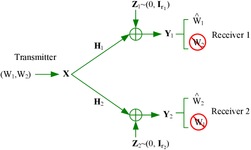
Figure 1: MIMO Gaussian broadcast channel with confidential messages.

Consider the communication scenario in which there are two independent messages $W_{1}$ and $W_{2}$ at the transmitter. Message $W_{1}$ is intended for receiver 1 but needs to be kept secret from receiver 2, and message $W_{2}$ is intended for receiver 1 but needs to be kept secret from receiver 2. (See Fig. 1 for an illustration of this communication scenario.) The confidentiality of the messages at the unintended receivers is measured using the normalized information-theoretic quantities [1, 2]:

$$\frac{1}{n}I(W_{1};\mathbf{Y}_{2}^{n})\rightarrow 0\quad\mbox{and}\quad\frac{1}{n}I(W_{2};\mathbf{Y}_{1}^{n})\rightarrow 0$$

where $\mathbf{Y}_{k}^{n}:=(\mathbf{Y}_{k}[1],\ldots,\mathbf{Y}_{k}[n])$, and the limits are taken as the block length $n\rightarrow\infty$. The goal is to characterize the entire secrecy rate region ${\mathcal{C}}_{s}(\mathbf{H}_{1},\mathbf{H}_{2},\mathbf{S})=\{(R_{1},R_{2})\}$ that can be achieved by any coding scheme. ${\mathcal{C}}_{s}(\mathbf{H}_{1},\mathbf{H}_{2},\mathbf{S})$ is usually known as the secrecy capacity region of the channel.

In recent years, information-theoretic study of secret MIMO communication has been an active area of research. (See [3] for a recent survey of progress in this area.) Most noticeably, the secrecy capacity of the MIMO Gaussian wiretap channel was characterized in [4, 5, 6] for the multiple-input single-output (MISO) case and [7, 8, 9, 10] for the general MIMO case. The secrecy capacity region of the MIMO Gaussian broadcast channel with a common and a confidential messages was characterized in [11]. The problem of communicating two confidential messages over the two-receiver MIMO Gaussian broadcast channel was first considered in [12], where it was shown that under the average total power constraint, secret dirty-paper coding (S-DPC) based on double binning [13] achieves the secrecy capacity region for the MISO case. For the general MIMO case, however, characterizing the secrecy capacity region remained as an open problem.

The main result of this paper is a precise characterization of the secrecy capacity region of the (general) MIMO Gaussian broadcast channel, summarized in the following theorem.

Theorem 1

The secrecy capacity region ${\mathcal{C}}_{s}(\mathbf{H}_{1},\mathbf{H}_{2},\mathbf{S})$ of the MIMO Gaussian broadcast channel (1) with confidential messages $W_{1}$ (intended for receiver 1 but needing to be kept secret from receiver 2) and $W_{2}$ (intended for receiver 2 but needing to be kept secret from receiver 1) under the matrix power constraint (2) is given by the set of nonnegative rate pairs $(R_{1},R_{2})$ such that

$$R_{1} \leq\max_{0\preceq\mathbf{B}\preceq\mathbf{S}}\left(\frac{1}{2}\log\left|\mathbf{I}_{r_{1}}+\mathbf{H}_{1}\mathbf{B}\mathbf{H}_{1}^{\intercal}\right|-\frac{1}{2}\log\left|\mathbf{I}_{r_{2}}+\mathbf{H}_{2}\mathbf{B}\mathbf{H}_{2}^{\intercal}\right|\right)$$

$$\text{and}\qquad R_{2} \leq\max_{0\preceq\mathbf{B}\preceq\mathbf{S}}\left(\frac{1}{2}\log\left|\frac{\mathbf{I}_{r_{2}}+\mathbf{H}_{2}\mathbf{S}\mathbf{H}_{2}^{\intercal}}{\mathbf{I}_{r_{2}}+\mathbf{H}_{2}\mathbf{B}\mathbf{H}_{2}^{\intercal}}\right|-\frac{1}{2}\log\left|\frac{\mathbf{I}_{r_{1}}+\mathbf{H}_{1}\mathbf{S}\mathbf{H}_{1}^{\intercal}}{\mathbf{I}_{r_{1}}+\mathbf{H}_{1}\mathbf{B}\mathbf{H}_{1}^{\intercal}}\right|\right)$$ (3)

where $\mathbf{I}_{r_{k}}$ denotes the identity matrix of size $r_{k}\times r_{k}$.

Remark 1

Note that the rate region (3) is rectangular. This implies that under the matrix power constraint, both confidential messages $W_{1}$ and $W_{2}$ can be simultaneously transmitted at their respective maximal secrecy rates (as if over two separate MIMO Gaussian wiretap channels). The secrecy capacity of the MIMO Gaussian wiretap channel under the matrix power constraint was characterized in [9], by which the rate region (3) can be rewritten as the set of nonnegative rate pairs $(R_{1},R_{2})$ such that

$$R_{1} \leq\max_{0\preceq\mathbf{B}\preceq\mathbf{S}}\left(\frac{1}{2}\log\left|\mathbf{I}_{r_{1}}+\mathbf{H}_{1}\mathbf{B}\mathbf{H}_{1}^{\intercal}\right|-\frac{1}{2}\log\left|\mathbf{I}_{r_{2}}+\mathbf{H}_{2}\mathbf{B}\mathbf{H}_{2}^{\intercal}\right|\right)$$

$$\text{and}\qquad R_{2} \leq\max_{0\preceq\mathbf{B}\preceq\mathbf{S}}\left(\frac{1}{2}\log\left|\mathbf{I}_{r_{2}}+\mathbf{H}_{2}\mathbf{B}\mathbf{H}_{2}^{\intercal}\right|-\frac{1}{2}\log\left|\mathbf{I}_{r_{1}}+\mathbf{H}_{1}\mathbf{B}\mathbf{H}_{1}^{\intercal}\right|\right).$$ (4)

Remark 2

Also note that if $\mathbf{B}^{\star}$ is an optimal solution to the optimization program:

$$\max_{0\preceq\mathbf{B}\preceq\mathbf{S}}\left(\log\left|\mathbf{I}_{r_{1}}+\mathbf{H}_{1}\mathbf{B}\mathbf{H}_{1}^{\intercal}\right|-\log\left|\mathbf{I}_{r_{2}}+\mathbf{H}_{2}\mathbf{B}\mathbf{H}_{2}^{\intercal}\right|\right),$$ (5)

then $\mathbf{B}^{\star}$ simultaneously maximizes both objective functions on the right-hand side (RHS) of (3). On the other hand, the optimization programs on the RHS of (4) do not, in general, admit the same optimal solution. As we will see, this makes (3) a better choice when it comes to proving the achievability part of the theorem.

It is rather surprising to see that under the matrix power constraint, both confidential messages $W_{1}$ and $W_{2}$ can be simultaneously transmitted at their respective maximal secrecy rates over the MIMO Gaussian broadcast channel (1). As we will see, this is due to the fact that there are in fact two different coding schemes: one uses only random binning, and the other uses both random binning and artificial noise. Both of them can achieve the secrecy capacity of the MIMO Gaussian wiretap channel. Through S-DPC (double binning) [13], both schemes can be simultaneously implemented in communicating confidential messages $W_{1}$ and $W_{2}$ over the MIMO Gaussian broadcast channel (1).

As a corollary, we have the following characterization of the secrecy capacity region under the average total power constraint. The result is a simple consequence of [14, Lemma 1].

Corollary 1

The secrecy capacity region ${\mathcal{C}}_{s}(\mathbf{H}_{1},\mathbf{H}_{2},P)$ of the MIMO Gaussian broadcast channel (1) with confidential messages $W_{1}$ (intended for receiver 1 but needing to be kept secret from receiver 2) and $W_{2}$ (intended for receiver 2 but needing to be kept secret from receiver 1) under the average total power constraint:

$$\frac{1}{n}\sum_{m=1}^{n}\|\mathbf{X}[m]\|^{2}\leq P$$ (6)

is given by the set of nonnegative rate pairs $(R_{1},R_{2})$ such that

$$R_{1} \leq\frac{1}{2}\log\left|\mathbf{I}_{r_{1}}+\mathbf{H}_{1}\mathbf{B}_{1}\mathbf{H}_{1}^{\intercal}\right|-\frac{1}{2}\log\left|\mathbf{I}_{r_{2}}+\mathbf{H}_{2}\mathbf{B}_{1}\mathbf{H}_{2}^{\intercal}\right|$$

$$\mbox{and}\quad\quad R_{2} \leq\frac{1}{2}\log\left|\frac{\mathbf{I}_{r_{2}}+\mathbf{H}_{2}(\mathbf{B}_{1}+\mathbf{B}_{2})\mathbf{H}_{2}^{\intercal}}{\mathbf{I}_{r_{2}}+\mathbf{H}_{2}\mathbf{B}_{1}\mathbf{H}_{2}^{\intercal}}\right|-\frac{1}{2}\log\left|\frac{\mathbf{I}_{r_{1}}+\mathbf{H}_{1}(\mathbf{B}_{1}+\mathbf{B}_{2})\mathbf{H}_{1}^{\intercal}}{\mathbf{I}_{r_{1}}+\mathbf{H}_{1}\mathbf{B}_{1}\mathbf{H}_{1}^{\intercal}}\right|$$ (7)

for some positive semidefinite matrices $\mathbf{B}_{1}$ and $\mathbf{B}_{2}$ such that ${\sf Tr}(\mathbf{B}_{1}+\mathbf{B}_{2})\leq{P}$.

Remark 3

Unlike Theorem 1, under the average total power constraint, the secrecy capacity region of the MIMO Gaussian broadcast channel is, in general, not rectangular.

The rest of the paper is devoted to the proof of Theorem 1. As mentioned previously, the rectangular nature of the rate region (3) suggests that the result is intimately connected to the secrecy capacity of the MIMO Gaussian wiretap channel. The secrecy capacity of the MIMO Gaussian wiretap channel under the matrix power constraint was previously characterized in [9], where it was shown that Gaussian random binning without prefix coding is optimal. In Section II, we revisit the MIMO Gaussian wiretap channel problem and show that Gaussian random binning with prefix coding can also achieve the secrecy capacity, provided that the prefix channel is appropriately chosen. In Section III, we prove Theorem 1 using two different characterizations of the secrecy capacity of the MIMO Gaussian wiretap channel and S-DPC (double binning) [13]. Numerical examples are provided in Section IV to illustrate the theoretical results. Finally, in Section V, we conclude the paper with some remarks.

II MIMO Gaussian Wiretap Channel Revisited

In this section, we revisit the problem of the MIMO Gaussian wiretap channel under a matrix power constraint. The problem was first considered in [9], where a precise characterization of the secrecy capacity was provided. The goal of this section is to provide an alternative characterization of the secrecy capacity which will facilitate proving Theorem 1. More specifically, we wish to provide a MIMO wiretap channel bound on the secrecy rate $R_{2}$ which will match the RHS of (3).

For that purpose, consider again the MIMO Gaussian broadcast channel (1) but this time with only one confidential message $W$ at the transmitter. Message $W$ is intended for receiver 2 (the legitimate receiver) but needs to be kept secret from receiver 1 (the eavesdropper). The confidentiality of $W$ at receiver 1 is measured using the normalized information-theoretic quantity [1, 2]:

$$\frac{1}{n}I(W;\mathbf{Y}_{1}^{n})\rightarrow 0.$$

The channel input $\{\mathbf{X}[m]\}_{m}$ is subject to the matrix power constraint (2). The goal is to characterize the secrecy capacity $C_{s}(\mathbf{H}_{2},\mathbf{H}_{1},\mathbf{S})$, which is the maximum achievable secrecy rate for message $W$. This communication scenario, as illustrated in Fig. 2, is widely known as the MIMO Gaussian wiretap channel [4, 6, 5, 7, 8, 9].

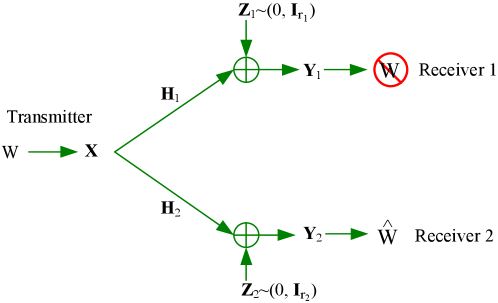
Figure 2: MIMO Gaussian wiretap channel.

In their seminal work [2], Csiszár and Körner provided a single-letter characterization of the secrecy capacity:

$$C_{s}(\mathbf{H}_{2},\mathbf{H}_{1},\mathbf{S})=\max_{(U,\mathbf{X})}\left[I(U;\mathbf{Y}_{2})-I(U;\mathbf{Y}_{1})\right]$$ (8)

where $U$ is an auxiliary variable, and the maximization is over all jointly distributed $(U,\mathbf{X})$ such that $U\rightarrow\mathbf{X}\rightarrow(\mathbf{Y}_{1},\mathbf{Y}_{2})$ forms a Markov chain and ${\sf E}[\mathbf{X}\mathbf{X}^{\intercal}]\preceq\mathbf{S}$. Here, $I(U,\mathbf{Y}_{k})$ denotes the mutual information between $U$ and $\mathbf{Y}_{k}$. As shown in [2], the secrecy rate on the RHS of (8) can be achieved by a coding scheme that combines random binning and prefix coding [2]. More specifically, the auxiliary variable $U$ represents a precoding signal, and the conditional distribution of $\mathbf{X}$ given $U$ represents the prefix channel. In [9], Liu and Shamai further studied the optimization problem on the RHS of (8) and showed that a Gaussian $U=\mathbf{X}$ is an optimal solution. Hence, a matrix characterization of the secrecy capacity is given by [9]

$$C_{s}(\mathbf{H}_{2},\mathbf{H}_{1},\mathbf{S})=\max_{0\preceq\mathbf{B}\preceq\mathbf{S}}\left(\frac{1}{2}\log\left|\mathbf{I}_{r_{2}}+\mathbf{H}_{2}\mathbf{B}\mathbf{H}_{2}^{\intercal}\right|-\frac{1}{2}\log\left|\mathbf{I}_{r_{1}}+\mathbf{H}_{1}\mathbf{B}\mathbf{H}_{1}^{\intercal}\right|\right).$$ (9)

We may conclude that Gaussian random binning without prefix coding is an optimal coding strategy for the MIMO Gaussian wiretap channel.

Next, we show that a different coding scheme that combines Gaussian random binning and prefix coding can also achieve the secrecy capacity of the MIMO Gaussian wiretap channel. This leads to a new characterization of the secrecy capacity, summarized in the following theorem.

Theorem 2

The secrecy capacity $C_{s}(\mathbf{H}_{2},\mathbf{H}_{1},\mathbf{S})$ of the MIMO Gaussian broadcast channel (1) with a confidential message $W$ (intended for receiver 2 but needing to be kept secret from receiver 1) under the matrix power constraint (2) is given by:

$$C_{s}(\mathbf{H}_{2},\mathbf{H}_{1},\mathbf{S})=\max_{0\preceq\mathbf{B}\preceq\mathbf{S}}\left(\frac{1}{2}\log\left|\frac{\mathbf{I}_{r_{2}}+\mathbf{H}_{2}\mathbf{S}\mathbf{H}_{2}^{\intercal}}{\mathbf{I}_{r_{2}}+\mathbf{H}_{2}\mathbf{B}\mathbf{H}_{2}^{\intercal}}\right|-\frac{1}{2}\log\left|\frac{\mathbf{I}_{r_{1}}+\mathbf{H}_{1}\mathbf{S}\mathbf{H}_{1}^{\intercal}}{\mathbf{I}_{r_{1}}+\mathbf{H}_{1}\mathbf{B}\mathbf{H}_{1}^{\intercal}}\right|\right).$$ (10)

Remark 4

The achievability of the secrecy rate on the RHS of (10) can be obtained from the Csiszár-Körner expression (8) by choosing $\mathbf{X}=U+V$, where $U$ and $V$ are two independent Gaussian vectors with zero means and covariance matrices $\mathbf{S}-\mathbf{B}$ and $\mathbf{B}$, respectively. This choice of $(U,\mathbf{X})$ differs from that for (9) in two important ways:

1. In (10), the input vector $\mathbf{X}$ always has a full covariance matrix $\mathbf{S}$. For (9), the covariance matrix of $\mathbf{X}$ needs to be chosen to solve an optimization program; the full covariance matrix $\mathbf{S}$ is not always an optimal solution.

2. In (10), the conditional distribution of $\mathbf{X}$ given $U$ may form a nontrivial prefix channel. For (9), $U\equiv\mathbf{X}$ so prefix coding is never applied.

Remark 5

Note that the prefix channel in (10) is an additive vector Gaussian noise channel, so the auxiliary variable $V$ represents an artificial noise [15] sent (on purpose) by the transmitter to confuse the eavesdropper. Since the artificial noise has no structure to it, it will add to the noise floor at both legitimate receiver and the eavesdropper.

The converse part of the theorem can be proved using a channel-enhancement argument, similar to that in [9]. The details of the proof are provided in Appendix A.

III MIMO Gaussian Broadcast Channel with Confidential Messages

In this section, we prove Theorem 1. To prove the converse part of the theorem, we will consider a single-message, wiretap channel bound on the secrecy rates $R_{1}$ and $R_{2}$. More specifically, note that both messages $W_{1}$ and $W_{2}$ can be transmitted at the maximum secrecy rate when the other message is absent from the transmission. Therefore, to bound from above the secrecy rate $R_{1}$, we assume that only $W_{1}$ needs to be communicated over the channel. This is precisely a MIMO Gaussian wiretap channel problem with receiver 1 as legitimate receiver and receiver 2 as eavesdropper. Reversing the roles of receiver 1 and 2, we have from (9) that

$$R_{1} \leq C_{s}(\mathbf{H}_{1},\mathbf{H}_{2},\mathbf{S})$$

$$=\max_{0\preceq\mathbf{B}\preceq\mathbf{S}}\left(\frac{1}{2}\log\left|\mathbf{I}_{r_{1}}+\mathbf{H}_{1}\mathbf{B}\mathbf{H}_{1}^{\intercal}\right|-\frac{1}{2}\log\left|\mathbf{I}_{r_{2}}+\mathbf{H}_{2}\mathbf{B}\mathbf{H}_{2}^{\intercal}\right|\right).$$ (11)

Similarly, to bound from above the secrecy rate $R_{2}$, let us assume that only $W_{2}$ needs to be communicated over the channel. This is, again, a MIMO Gaussian wiretap channel problem with receiver 2 playing the role of legitimate receiver and receiver 1 playing the role of eavesdropper. By Theorem 2,

$$R_{2} \leq C_{s}(\mathbf{H}_{2},\mathbf{H}_{1},\mathbf{S})$$

$$=\max_{0\preceq\mathbf{B}\preceq\mathbf{S}}\left(\frac{1}{2}\log\left|\frac{\mathbf{I}_{r_{2}}+\mathbf{H}_{2}\mathbf{S}\mathbf{H}_{2}^{\intercal}}{\mathbf{I}_{r_{2}}+\mathbf{H}_{2}\mathbf{B}\mathbf{H}_{2}^{\intercal}}\right|-\frac{1}{2}\log\left|\frac{\mathbf{I}_{r_{1}}+\mathbf{H}_{1}\mathbf{S}\mathbf{H}_{1}^{\intercal}}{\mathbf{I}_{r_{1}}+\mathbf{H}_{1}\mathbf{B}\mathbf{H}_{1}^{\intercal}}\right|\right).$$ (12)

Putting together (11) and (12), we have proved the converse part of the theorem.

Next, we show that every rate pair $(R_{1},R_{2})$ within the secrecy rate region (3) is achievable. Note that (3) is rectangular, so we only need to show that the corner point $(R_{1},R_{2})$ given by

$$R_{1} =\max_{0\preceq\mathbf{B}\preceq\mathbf{S}}\left(\frac{1}{2}\log\left|\mathbf{I}_{r_{1}}+\mathbf{H}_{1}\mathbf{B}\mathbf{H}_{1}^{\intercal}\right|-\frac{1}{2}\log\left|\mathbf{I}_{r_{2}}+\mathbf{H}_{2}\mathbf{B}\mathbf{H}_{2}^{\intercal}\right|\right)$$

$$\text{and}\qquad R_{2} =\max_{0\preceq\mathbf{B}\preceq\mathbf{S}}\left(\frac{1}{2}\log\left|\frac{\mathbf{I}_{r_{2}}+\mathbf{H}_{2}\mathbf{S}\mathbf{H}_{2}^{\intercal}}{\mathbf{I}_{r_{2}}+\mathbf{H}_{2}\mathbf{B}\mathbf{H}_{2}^{\intercal}}\right|-\frac{1}{2}\log\left|\frac{\mathbf{I}_{r_{1}}+\mathbf{H}_{1}\mathbf{S}\mathbf{H}_{1}^{\intercal}}{\mathbf{I}_{r_{1}}+\mathbf{H}_{1}\mathbf{B}\mathbf{H}_{1}^{\intercal}}\right|\right)$$ (13)

is achievable.

Recall from [13] that for any jointly distributed $(V_{1},V_{2},\mathbf{X})$ such that $(V_{1},V_{2})\rightarrow\mathbf{X}\rightarrow(\mathbf{Y}_{1},\mathbf{Y}_{2})$ forms a Markov chain and ${\sf E}[\mathbf{X}\mathbf{X}^{\intercal}]\preceq\mathbf{S}$, the secrecy rate pair $(R_{1},R_{2})$ given by

$$R_{1} =I(V_{1};\mathbf{Y}_{1})-I(V_{1};V_{2},\mathbf{Y}_{2})$$

$$\text{and}\qquad R_{2} =I(V_{2};\mathbf{Y}_{2})-I(V_{2};V_{1},\mathbf{Y}_{1})$$ (14)

is achievable for the MIMO Gaussian broadcast channel (1) under the matrix power constraint (2). In [13], the achievability of the rate pair (14) was proved using a double-binning scheme. Specifically, the auxiliary variables $V_{1}$ and $V_{2}$ represent the precoding signals for the confidential messages $W_{1}$ and $W_{2}$, respectively.

Now let $\mathbf{B}$ be a positive semidefinite matrix such that $\mathbf{B}\preceq\mathbf{S}$, and let

$$V_{1} =\mathbf{U}_{1}+\mathbf{F}\mathbf{U}_{2}$$

$$V_{2} =\mathbf{U}_{2}$$

$$\mbox{and}\quad\quad\mathbf{X} =\mathbf{U}_{1}+\mathbf{U}_{2}$$ (15)

where $\mathbf{U}_{1}$ and $\mathbf{U}_{2}$ are two independent Gaussian vectors with zero means and covariance matrices $\mathbf{B}$ and $\mathbf{S}-\mathbf{B}$, respectively, and

$$\mathbf{F} :=\mathbf{B}\mathbf{H}_{1}^{\intercal}(\mathbf{I}_{r_{1}}+\mathbf{H}_{1}\mathbf{B}\mathbf{H}_{1}^{\intercal})^{-1}\mathbf{H}_{1}.$$ (16)

By (15),

$$\mathbf{Y}_{k}=\mathbf{H}_{k}(\mathbf{U}_{1}+\mathbf{U}_{2})+\mathbf{Z}_{k}$$

for $k=1,2$. Note that the matrix $\mathbf{F}$ defined in (16) is precisely the precoding matrix for suppressing $\mathbf{U}_{2}$ from $\mathbf{Y}_{1}$ [16, Theorem 1]. Hence,

$$I(V_{1};\mathbf{Y}_{1})-I(V_{1};V_{2}) =I(V_{1};\mathbf{Y}_{1})-I(V_{1};\mathbf{U}_{2})$$

$$=\frac{1}{2}\log\left|\mathbf{I}_{r_{1}}+\mathbf{H}_{1}\mathbf{B}\mathbf{H}_{1}^{\intercal}\right|.$$ (17)

Moreover,

$$I(V_{1};\mathbf{Y}_{2}|V_{2}) =I(\mathbf{U}_{1}+\mathbf{F}\mathbf{U}_{2};\mathbf{H}_{2}(\mathbf{U}_{1}+\mathbf{U}_{2})+\mathbf{Z}_{2}|\mathbf{U}_{2})$$

$$=I(\mathbf{U}_{1};\mathbf{H}_{2}\mathbf{U}_{1}+\mathbf{Z}_{2}|\mathbf{U}_{2})$$

$$=I(\mathbf{U}_{1};\mathbf{H}_{2}\mathbf{U}_{1}+\mathbf{Z}_{2})$$

$$=\frac{1}{2}\log\left|\mathbf{I}_{r_{2}}+\mathbf{H}_{2}\mathbf{B}\mathbf{H}_{2}^{\intercal}\right|$$ (18)

where the third equality follows from the fact that $\mathbf{U}_{1}$ and $\mathbf{U}_{2}$ are independent. Putting together (17) and (18), we have

$$I(V_{1};\mathbf{Y}_{1})-I(V_{1};V_{2},\mathbf{Y}_{2}) =[I(V_{1};\mathbf{Y}_{1})-I(V_{1};V_{2})]-I(V_{1};\mathbf{Y}_{2}|V_{2})$$

$$=\frac{1}{2}\log\left|\mathbf{I}_{r_{1}}+\mathbf{H}_{1}\mathbf{B}\mathbf{H}_{1}^{\intercal}\right|-\frac{1}{2}\log\left|\mathbf{I}_{r_{2}}+\mathbf{H}_{2}\mathbf{B}\mathbf{H}_{2}^{\intercal}\right|.$$ (19)

Similarly,

$$I(V_{1},V_{2};\mathbf{Y}_{1}) =I(\mathbf{U}_{1}+\mathbf{F}\mathbf{U}_{2},\mathbf{U}_{2};\mathbf{H}_{1}(\mathbf{U}_{1}+\mathbf{U}_{2})+\mathbf{Z}_{2})$$

$$=I(\mathbf{U}_{1},\mathbf{U}_{2};\mathbf{H}_{1}(\mathbf{U}_{1}+\mathbf{U}_{2})+\mathbf{Z}_{2})$$

$$=\frac{1}{2}\log\left|\mathbf{I}_{r_{1}}+\mathbf{H}_{1}\mathbf{S}\mathbf{H}_{1}^{\intercal}\right|.$$ (20)

Thus,

$$I(V_{2};V_{1},\mathbf{Y}_{1}) =I(V_{2};\mathbf{Y}_{1}|V_{1})+I(V_{2};V_{1})$$

$$=I(V_{1},V_{2};\mathbf{Y}_{1})-[I(V_{1};\mathbf{Y}_{1})-I(V_{1};V_{2})]$$

$$=\frac{1}{2}\log\left|\frac{\mathbf{I}_{r_{1}}+\mathbf{H}_{1}\mathbf{S}\mathbf{H}_{1}^{\intercal}}{\mathbf{I}_{r_{1}}+\mathbf{H}_{1}\mathbf{B}\mathbf{H}_{1}^{\intercal}}\right|$$ (21)

where the last equality follows from (17) and (20). Moreover,

$$I(V_{2};\mathbf{Y}_{2}) =I(\mathbf{U}_{2};\mathbf{H}_{2}(\mathbf{U}_{1}+\mathbf{U}_{2})+\mathbf{Z}_{2})$$

$$=\frac{1}{2}\log\left|\frac{\mathbf{I}_{r_{2}}+\mathbf{H}_{2}\mathbf{S}\mathbf{H}_{2}^{\intercal}}{\mathbf{I}_{r_{2}}+\mathbf{H}_{2}\mathbf{B}\mathbf{H}_{2}^{\intercal}}\right|.$$ (22)

Putting together (21) and (22), we have

$$I(V_{2};\mathbf{Y}_{2})-I(V_{2};V_{1},\mathbf{Y}_{1}) =\frac{1}{2}\log\left|\frac{\mathbf{I}_{r_{2}}+\mathbf{H}_{2}\mathbf{S}\mathbf{H}_{2}^{\intercal}}{\mathbf{I}_{r_{2}}+\mathbf{H}_{2}\mathbf{B}\mathbf{H}_{2}^{\intercal}}\right|-\frac{1}{2}\log\left|\frac{\mathbf{I}_{r_{1}}+\mathbf{H}_{1}\mathbf{S}\mathbf{H}_{1}^{\intercal}}{\mathbf{I}_{r_{1}}+\mathbf{H}_{1}\mathbf{B}\mathbf{H}_{1}^{\intercal}}\right|.$$ (23)

Finally, let $\mathbf{B}$ be an optimal solution to the optimization program (5). As mentioned previously in Remark 2, such a choice will simultaneously maximize the RHS of (19) and (23). Thus, the corner point (13) is indeed achievable. This completes the proof of the theorem.

Remark 6

Note that in standard dirty-paper coding (DPC), the precoding matrix $\mathbf{F}$ is chosen to cancel the known interference. In our scheme, such a choice plays two important roles. First, it helps to cancel the precoding signal representing message $W_{2}$, so message $W_{1}$ sees an interference-free legitimate receiver channel. Second, it helps to boost the security for message $W_{2}$ by causing interference to its eavesdropper. For this reason, we call our scheme S-DPC, to differentiate from the standard DPC.

Remark 7

In S-DPC, both the legitimate receiver and the eavesdropper for message $W_{1}$ are interference free. On the other hand, for message $W_{2}$, both the legitimate receiver and the eavesdropper are subject to interference from the precoding signal representing message $W_{1}$. As we have seen in Section II, the secrecy capacity of the MIMO Gaussian wiretap channel can be achieved with or without interference in place. Therefore, both secrecy capacity achieving schemes can be simultaneously implemented via S-DPC to simultaneously communicate both confidential messages at their respective maximal secrecy rates.

IV Numerical Examples

In this section, we provide numerical examples to illustrate the secrecy capacity region of the MIMO Gaussian wiretap channel with confidential messages. As shown in (3) and (7), under both matrix and average total power constraints, the secrecy capacity regions ${\mathcal{C}}_{s}(\mathbf{H}_{1},\mathbf{H}_{2},\mathbf{S})$ and ${\mathcal{C}}_{s}(\mathbf{H}_{1},\mathbf{H}_{2},P)$ are expressed in terms of matrix optimization programs (though implicit in (7)). In general, these optimization programs are not convex, and hence, finding the boundary of the secrecy capacity regions is nontrivial.

In [12], a precise characterization of the secrecy capacity region ${\mathcal{C}}_{s}(\mathbf{H}_{1},\mathbf{H}_{2},P)$ was obtained for the MISO Gaussian broadcast channel using the generalized eigenvalue decomposition [17, Ch. 6.3]. For the aligned MIMO Gaussian wiretap channel, [10] provided an explicit, closed-form expression for the secrecy capacity. In the following, we generalize the results of [10] and [12] to the general MIMO Gaussian broadcast channel under the matrix power constraint.

Let $\phi_{j}$, $j=1,\ldots,t$, be the generalized eigenvalues of the pencil

$$\left(\mathbf{I}_{t}+\mathbf{S}^{\frac{1}{2}}\mathbf{H}_{1}^{\intercal}\mathbf{H}_{1}\mathbf{S}^{\frac{1}{2}},\;\mathbf{I}_{t}+\mathbf{S}^{\frac{1}{2}}\mathbf{H}_{2}^{\intercal}\mathbf{H}_{2}\mathbf{S}^{\frac{1}{2}}\right).$$ (24)

Since both $\mathbf{I}_{t}+\mathbf{S}^{\frac{1}{2}}\mathbf{H}_{1}^{\intercal}\mathbf{H}_{1}\mathbf{S}^{\frac{1}{2}}$ and $\mathbf{I}_{t}+\mathbf{S}^{\frac{1}{2}}\mathbf{H}_{2}^{\intercal}\mathbf{H}_{2}\mathbf{S}^{\frac{1}{2}}$ are strictly positive definite, we have $\phi_{j}>0$ for $j=1,\dots,t$. Without loss of generality, we may assume that these generalized eigenvalues are ordered as

$$\phi_{1}\geq\dots\geq\phi_{\rho}>1\geq\phi_{\rho+1}\geq\dots\geq\phi_{t}>0,$$

i.e., a total of $\rho$ of them are assumed to be greater than $1$. We have the following characterization of the secrecy capacity of the MIMO Gaussian wiretap channel under the matrix power constraint, which is a natural extension of [10].

Theorem 3

The secrecy capacity $C_{s}(\mathbf{H}_{1},\mathbf{H}_{2},\mathbf{S})$ of the MIMO Gaussian broadcast channel (1) with confidential message $W$ (intended for receiver 1 but needing to be kept secret from receiver 2) under the matrix power constraint (2) is given by

$$C_{s}(\mathbf{H}_{1},\mathbf{H}_{2},\mathbf{S})=\frac{1}{2}\sum_{j=1}^{\rho}\log\phi_{j}$$ (25)

where $\phi_{j}$, $j=1,\ldots,\rho$, are the generalized eigenvalues of the pencil (24) that are greater than 1.

Remark 8

Note that $\mathbf{I}_{t}+\mathbf{S}^{\frac{1}{2}}\mathbf{H}_{2}^{\intercal}\mathbf{H}_{2}\mathbf{S}^{\frac{1}{2}}$ is invertible, so computing the generalized eigenvalues of the pencil (24) can be reduced to the problem of finding standard eigenvalues of a related semidefinite matrix [17, Ch. 6.3]. Hence, the secrecy capacity expression (25) is computable.

A proof of the theorem following the approach of [10] is provided in Appendix B. As a corollary, we have the following characterization of the secrecy capacity region of the MIMO Gaussian broadcast channel with confidential messages under the matrix power constraint.

Corollary 2

The secrecy capacity region ${\mathcal{C}}_{s}(\mathbf{H}_{1},\mathbf{H}_{2},\mathbf{S})$ of the MIMO Gaussian broadcast channel (1) with confidential messages $W_{1}$ (intended for receiver 1 but needing to be kept secret from receiver 2) and $W_{2}$ (intended for receiver 2 but needing to be kept secret from receiver 1) under the matrix constraint (2) is given by the set of nonnegative rate pairs $(R_{1},R_{2})$ such that

$$R_{1} \leq\frac{1}{2}\sum_{j=1}^{\rho}\log\phi_{j}$$

$$\text{and}\qquad R_{2} \leq\frac{1}{2}\sum_{j=\rho+1}^{t}\log\frac{1}{\phi_{j}}$$ (26)

where $\phi_{j}$, $j=1,\ldots,\rho$, are the generalized eigenvalues of the pencil (24) that are greater than 1, and $\phi_{j}$, $j=\rho+1,\ldots,t$, are the generalized eigenvalues of the pencil (24) that are less than or equal to 1.

Proof:

By Theorem 1, we only need to show that the secrecy capacity

$$C_{s}(\mathbf{H}_{2},\mathbf{H}_{1},\mathbf{S})=\frac{1}{2}\sum_{j=\rho+1}^{t}\log\frac{1}{\phi_{j}}.$$

Consider the pencil

$$\left(\mathbf{I}_{t}+\mathbf{S}^{\frac{1}{2}}\mathbf{H}_{2}^{\intercal}\mathbf{H}_{2}\mathbf{S}^{\frac{1}{2}},\;\mathbf{I}_{t}+\mathbf{S}^{\frac{1}{2}}\mathbf{H}_{1}^{\intercal}\mathbf{H}_{1}\mathbf{S}^{\frac{1}{2}}\right).$$ (27)

Note that the pencils (24) and (27) are generated by the same pair of semidefinite matrices but with different order. Therefore, the generalized eigenvalues of the pencil (27) are given by

$$0<\frac{1}{\phi_{1}}\leq\dots\leq\frac{1}{\phi_{\rho}}<1\leq\frac{1}{\phi_{\rho+1}}\leq\dots\leq\frac{1}{\phi_{t}}.$$

Applying Theorem 3 for $C_{s}(\mathbf{H}_{2},\mathbf{H}_{1},\mathbf{S})$ completes the proof of the corollary. ∎

Under the average total power constraint, we have not been able to find a computable secrecy capacity expression for the general MIMO case. We can, however, write [14, Lemma 1]

$${\mathcal{C}}_{s}(\mathbf{H}_{1},\mathbf{H}_{2},P)=\bigcup_{\mathbf{S}\succeq 0,\;{\sf Tr}(\mathbf{S})\leq P}{\mathcal{C}}_{s}(\mathbf{H}_{1},\mathbf{H}_{2},\mathbf{S}).$$

For any given semidefinite $\mathbf{S}$, ${\mathcal{C}}_{s}(\mathbf{H}_{1},\mathbf{H}_{2},\mathbf{S})$ can be computed as given by (26). Then, the secrecy capacity region ${\mathcal{C}}_{s}(\mathbf{H}_{1},\mathbf{H}_{2},P)$ can be found through an exhaustive search over the set $\{\mathbf{S}:\;\mathbf{S}\succeq 0\;\mbox{and}\;{\sf Tr}(\mathbf{S})\leq P\}$.

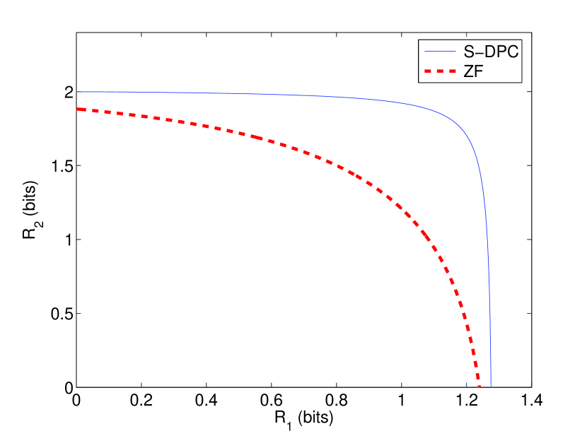
(a) $r_{1}=r_{2}=1$

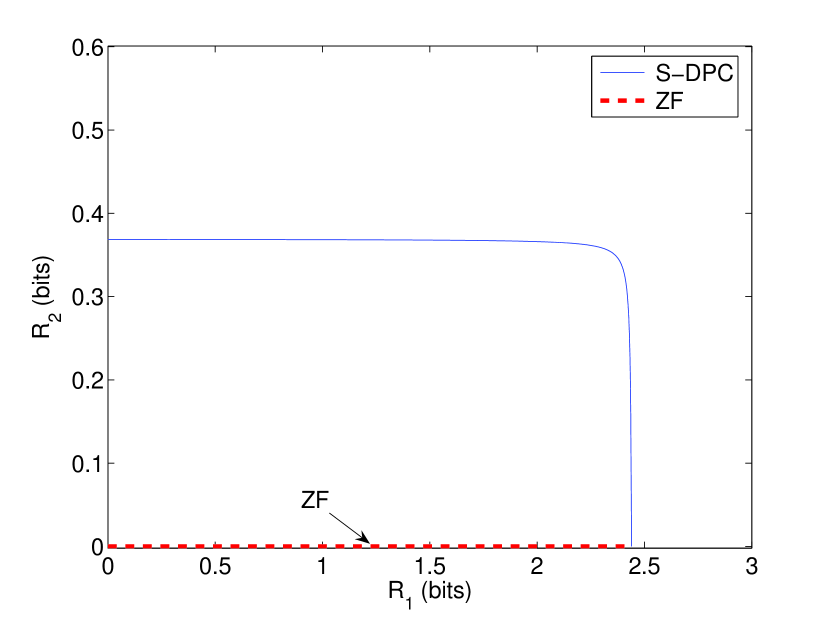
(b) $r_{1}=2$, $r_{2}=1$

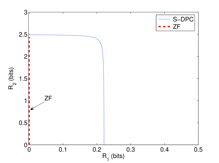
(c) $r_{1}=1$, $r_{2}=2$

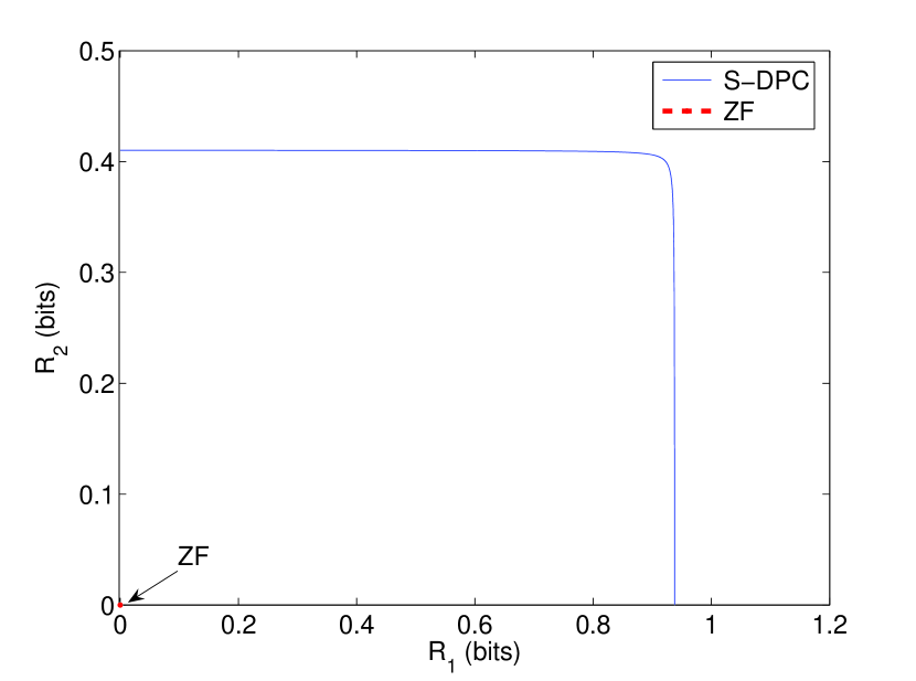
(d) $r_{1}=r_{2}=2$

Figure 3: Secrecy rate regions of the MIMO Gaussian broadcast channel under the average total power constraint.

Let $\mathbf{h}_{11}=(0.3\;2.5)$, $\mathbf{h}_{12}=(2.2\;1.8)$, $\mathbf{h}_{21}=(1.3\;1.2)$, $\mathbf{h}_{22}=(1.5\;3.9)$ and $P=12$, and let

$$\mathbf{H}_{k} =\left(\begin{array}[]{c}\mathbf{h}_{k1}\\ \mathbf{h}_{k2}\\ \end{array}\right),\quad k=1,2.$$

The secrecy capacity regions ${\mathcal{C}}_{s}(\mathbf{h}_{11},\mathbf{h}_{22},P)$, ${\mathcal{C}}_{s}(\mathbf{H}_{1},\mathbf{h}_{22},P)$, ${\mathcal{C}}_{s}(\mathbf{h}_{11},\mathbf{H}_{2},P)$ and ${\mathcal{C}}_{s}(\mathbf{H}_{1},\mathbf{H}_{2},P)$ are illustrated in Fig. 3. For comparison, we have also plotted the secrecy rate regions achieved by the simple zero-forcing (ZF) strategy. In ZF, each of the confidential messages is encoded using a vector Gaussian signal. To guarantee confidentiality, the covariance matrices of the transmit signals are chosen in the null space of the channel matrix at the unintended receiver. Hence, the achievable secrecy rate region is given by

$${\mathcal{R}}_{S}^{\rm ZF}(\mathbf{H}_{1},\mathbf{H}_{2},P)=\bigcup_{\begin{subarray}{c}\mathbf{B}_{1}\succeq 0,\;\mathbf{B}_{2}\succeq 0,\;{\sf Tr}(\mathbf{B}_{1}+\mathbf{B}_{2})\leq P\\ \mathbf{H}_{2}\mathbf{B}_{1}=0,\;\mathbf{H}_{1}\mathbf{B}_{2}=0\end{subarray}}\left\{(R_{1},R_{2})\left|\;\begin{array}[]{l}R_{1}\leq\frac{1}{2}\log|\mathbf{I}_{r_{1}}+\mathbf{H}_{1}\mathbf{B}_{1}\mathbf{H}_{1}^{\intercal}|\\ R_{2}\leq\frac{1}{2}\log|\mathbf{I}_{r_{2}}+\mathbf{H}_{2}\mathbf{B}_{2}\mathbf{H}_{2}^{\intercal}|\end{array}\right.\right\}.$$ (30)

Note that unlike the secrecy capacity region expression (7), computing the rate region (30) only involves solving convex optimization programs. As shown in Fig. 3, in all four scenarios, ZF is strictly suboptimal as compared with S-DPC. In particular, if the channel matrix of the unintended receiver has full row rank, ZF cannot achieve any positive secrecy rate for the corresponding confidential message. On the other hand, S-DPC can always achieve positive secrecy rates for both confidential messages unless the MIMO Gaussian broadcast channel is degraded.

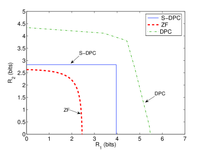
Figure 4: Rate regions of the MIMO Gaussian broadcast channel under the power matrix constraint.

Finally, let

$$\mathbf{H}_{1} =\left(\begin{matrix}1.8&-2.0&2.0\\ 1.0&-6.0&3.0\end{matrix}\right)$$

$$\mathbf{H}_{2} =\left(\begin{matrix}2.3&2.0&-3\\ 2.0&1.2&-1.5\end{matrix}\right)$$

and

$$\mathbf{S}=\left(\begin{matrix}5.0&-0.7&-2.0\\ -0.7&3.8&-2.5\\ -2.0&-2.5&5.0\end{matrix}\right).$$

Fig. 4 illustrates the secrecy capacity region $\mathcal{C}_{s}(\mathbf{H}_{1},\mathbf{H}_{2},\mathbf{S})$ of the MIMO Gaussian broadcast channel (1) under the matrix power constraint (2). Here, the secrecy capacity region $\mathcal{C}_{s}(\mathbf{H}_{1},\mathbf{H}_{2},\mathbf{S})$ is plotted based on the computable expression (26). Also in the figure are the secrecy rate region $\mathcal{R}_{s}^{\rm ZF}(\mathbf{H}_{1},\mathbf{H}_{2},\mathbf{S})$ achieved by ZF strategy and the nonsecrecy capacity region $\mathcal{R}^{\rm DPC}(\mathbf{H}_{1},\mathbf{H}_{2},\mathbf{S})$ achieved by standard DPC [14]. As expected, we have $\mathcal{R}_{s}^{\rm ZF}(\mathbf{H}_{1},\mathbf{H}_{2},\mathbf{S})\subset\mathcal{C}_{s}(\mathbf{H}_{1},\mathbf{H}_{2},\mathbf{S})\subset\mathcal{R}^{\rm DPC}(\mathbf{H}_{1},\mathbf{H}_{2},\mathbf{S})$.

V Concluding Remarks

In this paper, we have considered the problem of communicating two confidential messages over the two-receiver MIMO Gaussian broadcast channel. Each of the confidential messages is intended for one of the receivers but needs to be kept asymptotically perfectly secret from the other. Precise characterizations of the secrecy capacity region have been provided under both matrix and average total power constraints. Surprisingly, under the matrix power constraint, both confidential messages can be transmitted simultaneously at their respective maximal secrecy rates.

To prove this result, we have revisited the problem of the MIMO Gaussian wiretap channel and proposed a new coding scheme that achieves the secrecy capacity of the channel. Unlike the previous scheme considered in [4, 6, 5, 7, 8, 9] where prefix coding is not applied, the new coding scheme uses artificial vector Gaussian noise as a way of prefix coding. Moreover, the optimal covariance matrix of the artificial noise coincides with that of the transmit signal in the previous scheme. This allows both schemes to be overlayed via S-DPC without sacrificing the secrecy rate performance for either of them. We believe that the new understanding of the MIMO Gaussian wiretap channel problem gained in this work will help to solve some other multiuser secret communication problems.

Appendix A Proof of Theorem 2

In this appendix, we prove Theorem 2. As mentioned previously in Remark 4, the secrecy rate on the RHS of (10) can be achieved by a coding scheme that combines Gaussian random binning and prefix coding. We therefore concentrate on the converse part of the theorem.

Following [9], we will first prove the converse result for the special case where the channel matrices $\mathbf{H}_{1}$ and $\mathbf{H}_{2}$ are square and invertible. Next, we will broaden the result to the general case by approximating arbitrary channel matrices $\mathbf{H}_{1}$ and $\mathbf{H}_{2}$ by square and invertible ones. For brevity, we will term the special case as the aligned MIMO Gaussian wiretap channel and the general case as the general MIMO Gaussian wiretap channel.

A-A Aligned MIMO Gaussian Wiretap Channel

Consider the special case of the MIMO Gaussian broadcast channel (1) where the channel matrices $\mathbf{H}_{1}$ and $\mathbf{H}_{2}$ are square and invertible. Multiplying both sides of (1) by $\mathbf{H}_{k}^{-1}$, the channel model can be equivalently written as

$$\mathbf{Y}_{k}[m]=\mathbf{X}[m]+\mathbf{Z}_{k}[m],\quad k=1,2$$ (31)

where $\{\mathbf{Z}_{k}[m]\}_{m}$ is an i.i.d. additive vector Gaussian noise process with zero mean and covariance matrix

$$\mathbf{N}_{k} =\mathbf{H}_{k}^{-1}\mathbf{H}_{k}^{-\intercal}.$$ (32)

Denote by $C_{s}(\mathbf{N}_{2},\mathbf{N}_{1},\mathbf{S})$ the secrecy capacity of (31) (viewed as a MIMO Gaussian wiretap channel with receiver 2 as legitimate receiver and receiver 1 as eavesdropper) under the matrix power constraint (2). We have the following characterization of $C_{s}(\mathbf{N}_{2},\mathbf{N}_{1},\mathbf{S})$.

Lemma 1

The secrecy capacity

$$C_{s}(\mathbf{N}_{2},\mathbf{N}_{1},\mathbf{S}) =\max_{0\preceq\mathbf{B}\preceq\mathbf{S}}\left(\frac{1}{2}\log\left|\frac{\mathbf{S}+\mathbf{N}_{2}}{\mathbf{B}+\mathbf{N}_{2}}\right|-\frac{1}{2}\log\left|\frac{\mathbf{S}+\mathbf{N}_{1}}{\mathbf{B}+\mathbf{N}_{1}}\right|\right).$$ (33)

Proof:

The achievability of the secrecy rate on the RHS of (33) follows from the achievability of the secrecy rate on the RHS of (10) for the general case and the definition of $\mathbf{N}_{k}$ in (32). To prove the converse result, we will follow [9] and consider a channel-enhancement argument as follows.

Let us first assume that $\mathbf{S}\succ 0$. In this case, let $\mathbf{B}^{\star}$ be an optimal solution to the optimization program on the RHS of (33). Then, $\mathbf{B}^{\star}$ must satisfy the following Karush-Kuhn-Tucker conditions [9]:

$$(\mathbf{B}^{\star}+\mathbf{N}_{1})^{-1}+\mathbf{M}_{1} =(\mathbf{B}^{\star}+\mathbf{N}_{2})^{-1}+\mathbf{M}_{2}$$ (34a)

$$\mathbf{B}^{\star}\mathbf{M}_{1} =0$$ (34b)

$$\text{and}\quad\quad(\mathbf{S}-\mathbf{B}^{\star})\mathbf{M}_{2} =0$$ (34c)

where $\mathbf{M}_{1}$ and $\mathbf{M}_{2}$ are positive semidefinite matrices. Let $\widetilde{\mathbf{N}}_{1}$ be a real symmetric matrix such that

$$(\mathbf{B}^{\star}+\widetilde{\mathbf{N}}_{1})^{-1} =(\mathbf{B}^{\star}+\mathbf{N}_{1})^{-1}+\mathbf{M}_{1}.$$ (35)

From Eqns. (23), (25), (31) and (34) of [9], we have

$$0\prec\widetilde{\mathbf{N}}_{1}\preceq\{\mathbf{N}_{1},\mathbf{N}_{2}\},$$ (36)

$$\left|\frac{\mathbf{B}^{\star}+\widetilde{\mathbf{N}}_{1}}{\widetilde{\mathbf{N}}_{1}}\right|=\left|\frac{\mathbf{B}^{\star}+\mathbf{N}_{1}}{\mathbf{N}_{1}}\right|$$ (37)

and

$$\left|\frac{\mathbf{S}+\widetilde{\mathbf{N}}_{1}}{\mathbf{B}^{\star}+\widetilde{\mathbf{N}}_{1}}\right| =\left|\frac{\mathbf{S}+\mathbf{N}_{2}}{\mathbf{B}^{\star}+\mathbf{N}_{2}}\right|.$$ (38)

Now consider an enhanced MIMO Gaussian broadcast channel:

$$\mathbf{Y}_{1}[m] =\mathbf{X}[m]+\mathbf{Z}_{1}[m]$$

$$\text{and}\qquad\mathbf{Y}_{2}[m] =\mathbf{X}[m]+\tilde{\mathbf{Z}}_{1}[m]$$ (39)

where $\{\mathbf{Z}_{1}[m]\}_{m}$ and $\{\tilde{\mathbf{Z}}_{1}[m]\}_{m}$ are i.i.d. additive vector Gaussian noise processes with zero means and covariance matrices $\mathbf{N}_{1}$ and $\widetilde{\mathbf{N}}_{1}$, respectively. Denote by $C_{s}(\widetilde{\mathbf{N}}_{1},\mathbf{N}_{1},\mathbf{S})$ the secrecy capacity of (39) (viewed as a MIMO Gaussian wiretap channel with receiver 2 as legitimate receiver and receiver 1 as eavesdropper) under the matrix constraint (2). Note from (36) that $\widetilde{\mathbf{N}}_{1}\preceq\mathbf{N}_{1}$, so the enhanced MIMO Gaussian wiretap channel (39) is degraded. Hence,

$$C_{s}(\widetilde{\mathbf{N}}_{1},\mathbf{N}_{1},\mathbf{S}) =\frac{1}{2}\log\left|\frac{\mathbf{S}+\widetilde{\mathbf{N}}_{1}}{\widetilde{\mathbf{N}}_{1}}\right|-\frac{1}{2}\log\left|\frac{\mathbf{S}+\mathbf{N}_{1}}{\mathbf{N}_{1}}\right|$$

$$=\frac{1}{2}\log\left(\left|\frac{\mathbf{S}+\widetilde{\mathbf{N}}_{1}}{\mathbf{S}+\mathbf{N}_{1}}\right|\left|\frac{\mathbf{N}_{1}}{\widetilde{\mathbf{N}}_{1}}\right|\right)$$

$$=\frac{1}{2}\log\left(\left|\frac{\mathbf{S}+\widetilde{\mathbf{N}}_{1}}{\mathbf{S}+\mathbf{N}_{1}}\right|\left|\frac{\mathbf{B}^{\star}+\mathbf{N}_{1}}{\mathbf{B}^{\star}+\widetilde{\mathbf{N}}_{1}}\right|\right)$$

$$=\frac{1}{2}\log\left(\left|\frac{\mathbf{S}+\widetilde{\mathbf{N}}_{1}}{\mathbf{B}^{\star}+\widetilde{\mathbf{N}}_{1}}\right|\left|\frac{\mathbf{B}^{\star}+\mathbf{N}_{1}}{\mathbf{S}+\mathbf{N}_{1}}\right|\right)$$

$$=\frac{1}{2}\log\left(\left|\frac{\mathbf{S}+\mathbf{N}_{2}}{\mathbf{B}^{\star}+\mathbf{N}_{2}}\right|\left|\frac{\mathbf{B}^{\star}+\mathbf{N}_{1}}{\mathbf{S}+\mathbf{N}_{1}}\right|\right)$$

$$=\frac{1}{2}\log\left|\frac{\mathbf{S}+\mathbf{N}_{2}}{\mathbf{B}^{\star}+\mathbf{N}_{2}}\right|-\frac{1}{2}\log\left|\frac{\mathbf{S}+\mathbf{N}_{1}}{\mathbf{B}^{\star}+\mathbf{N}_{1}}\right|$$ (40)

where the first equality follows from [9, Theorem 1]; the third equality follows from (37); and the fifth equality follows from (38).

Finally, note from (36) that $\widetilde{\mathbf{N}}_{1}\preceq\mathbf{N}_{2}$, i.e., the legitimate receiver in the enhanced wiretap channel (39) receives a better signal that the legitimate receiver in the original wiretap channel (31). Therefore,

$$C_{s}(\mathbf{N}_{2},\mathbf{N}_{1},\mathbf{S}) \leq C_{s}(\widetilde{\mathbf{N}}_{1},\mathbf{N}_{1},\mathbf{S})$$

$$=\frac{1}{2}\log\left|\frac{\mathbf{S}+\mathbf{N}_{2}}{\mathbf{B}^{\star}+\mathbf{N}_{2}}\right|-\frac{1}{2}\log\left|\frac{\mathbf{S}+\mathbf{N}_{1}}{\mathbf{B}^{\star}+\mathbf{N}_{1}}\right|$$

where the last equality follows from (40). This proved the desired converse result for $\mathbf{S}\succ 0$.

For the case when $\mathbf{S}\succeq 0$, $|\mathbf{S}|=0$, let

$$\theta={\sf Rank}(\mathbf{S})<t.$$

Following the same footsteps as in the proof of [14, Lemma 2], we can define an equivalent aligned MIMO Gaussian wiretap channel with $\theta$ transmit and receive antennas and a new covariance matrix power constraint that is strictly positive definite. Hence, we can convert the case when $\mathbf{S}\succeq 0$, $|\mathbf{S}|=0$ to the case when $\mathbf{S}\succ 0$ with the same secrecy capacity. This argument can be formally described as follows.

Since $\mathbf{S}$ is positive semidefinite, we can write

$$\mathbf{S}=\mathbf{Q}_{\mathbf{S}}{\bf\Lambda_{\mathbf{S}}}\mathbf{Q}_{\mathbf{S}}^{\intercal}$$

where $\mathbf{Q}_{\mathbf{S}}$ is an orthogonal matrix and

$${\bf\Lambda_{\mathbf{S}}}={\sf Diag}(\underbrace{0,\dots,0}_{t-\theta},s_{1},\dots,s_{\theta})$$

is diagonal with $s_{j}>0$, $j=1,\dots,\theta$. For $k=1,2$, write

$$\mathbf{Q}_{\mathbf{S}}^{\intercal}\mathbf{N}_{k}\mathbf{Q}_{\mathbf{S}}=\left(\begin{matrix}\mathbf{C}_{k}&\mathbf{D}_{k}\\ \mathbf{D}_{k}^{\intercal}&\mathbf{E}_{k}\end{matrix}\right)$$

where $\mathbf{C}_{k}$, $\mathbf{D}_{k}$ and $\mathbf{E}_{k}$ are (sub)matrices of size $(t-\theta)\times(t-\theta)$, $(t-\theta)\times\theta$ and $\theta\times\theta$, respectively. Let

$$\mathbf{A}_{k}:=\left(\begin{matrix}\mathbf{I}_{t-\theta}&0_{(t-\theta)\times\theta}\\ -\mathbf{D}_{k}^{\intercal}\mathbf{C}_{k}^{-1}&\mathbf{I}_{\theta}\end{matrix}\right),\quad k=1,2.$$

We now define an intermediate and equivalent channel by multiplying both sides of (31) by an invertible matrix $\mathbf{A}_{k}\mathbf{Q}_{\mathbf{S}}^{\intercal}$:

$$\mathbf{Y}_{k}^{\prime}[m] =\mathbf{X}^{\prime}[m]+\mathbf{Z}_{k}^{\prime}[m],\quad k=1,2$$ (41)

where

$$\mathbf{Y}_{k}^{\prime}[m] =\mathbf{A}_{k}\mathbf{Q}_{\mathbf{S}}^{\intercal}\mathbf{Y}_{k}[m]$$

$$\mathbf{X}^{\prime}[m] =\mathbf{A}_{k}\mathbf{Q}_{\mathbf{S}}^{\intercal}\mathbf{X}[m]$$

$$\mbox{and}\quad\quad\mathbf{Z}_{k}^{\prime}[m] =\mathbf{A}_{k}\mathbf{Q}_{\mathbf{S}}^{\intercal}\mathbf{Z}_{k}[m].$$

Then, the covariance matrix $\mathbf{N}_{k}^{\prime}$ of the additive Gaussian noise vector $\mathbf{Z}_{k}^{\prime}[m]$ is given by

$$\mathbf{N}_{k}^{\prime} =\left(\begin{matrix}\mathbf{C}_{k}&0\\ 0&\mathbf{E}_{k}-\mathbf{D}_{k}^{\intercal}\mathbf{C}_{k}^{-1}\mathbf{D}_{k}\end{matrix}\right).$$ (42)

and the matrix power constraint (2) becomes

$$\frac{1}{n}\sum_{m=1}^{n}\mathbf{X}^{\prime}[m]{\mathbf{X}^{\prime}}^{\intercal}[m]\preceq\mathbf{S}^{\prime}$$ (43)

where

$$\mathbf{S}^{\prime} =\mathbf{A}_{k}\mathbf{Q}_{\mathbf{S}}^{\intercal}\mathbf{S}\mathbf{Q}_{\mathbf{S}}\mathbf{A}_{k}^{\intercal}$$

$$=\mathbf{A}_{k}{\bf\Lambda_{\mathbf{S}}}\mathbf{A}_{k}^{\intercal}$$

$$={\bf\Lambda_{\mathbf{S}}}.$$ (44)

Note from (44) that $\mathbf{S}^{\prime}$ is diagonal with first $t-\theta$ diagonal elements equal to zero. Thus, the matrix constraint (43) requires that the first $t-\theta$ elements of $\mathbf{X}^{\prime}[m]$ be zero. Moreover, from (42), the first $t-\theta$ and the rest of $\theta$ elements of $\mathbf{Z}^{\prime}_{k}[m]$ are uncorrelated and hence must be independent as $\mathbf{Z}^{\prime}_{k}[m]$ is Gaussian. Therefore, only the latter $\theta$ antennas transmit/receive information regarding message $W$. This allows us to define another equivalent aligned MIMO Gaussian broadcast channel with $\theta$ antennas at the transmitter and each of the receivers:

$$\overline{\mathbf{Y}}_{k}[m] =\overline{\mathbf{X}}[m]+\overline{\mathbf{Z}}_{k}[m],\quad k=1,2$$ (45)

where

$$\overline{\mathbf{Y}}_{k}[m] =\overline{\mathbf{A}}\mathbf{Y}^{\prime}_{k}[m]$$

$$\overline{\mathbf{X}}[m] =\overline{\mathbf{A}}\mathbf{X}^{\prime}[m]$$

$$\overline{\mathbf{Z}}_{k}[m] =\overline{\mathbf{A}}\mathbf{Z}^{\prime}_{k}[m]$$

and $\overline{\mathbf{A}}=\left[0_{\theta\times(t-\theta)}\;\mathbf{I}_{\theta}\right]$. Now, the matrix power constraint (43) becomes

$$\frac{1}{n}\sum_{m=1}^{n}\overline{\mathbf{X}}[m]\overline{\mathbf{X}}^{\intercal}[m]\preceq\overline{\mathbf{S}}$$ (46)

where

$$\overline{\mathbf{S}} =\overline{\mathbf{A}}\mathbf{S}^{\prime}\overline{\mathbf{A}}^{\intercal}$$

$$={\sf Diag}(s_{1},\dots,s_{\theta}).$$ (47)

Note that the matrix power constraint $\overline{\mathbf{S}}$ is strictly positive definite, so we can apply the previous result to the new wiretap channel (45). This completes the proof of the lemma. ∎

A-B General MIMO Gaussian Wiretap Channel

For the general case, we may assume that the channel matrices $\mathbf{H}_{1}$ and $\mathbf{H}_{2}$ are square but not necessarily invertible. If that is not the case, we can use singular value decomposition (SVD) to show that there is an equivalent channel which does have $t\times t$ square channel matrices. That is, we can find a new channel with square channel matrices which are derived from the original ones via matrix multiplications. The new channel is equivalent to the original one in preserving the secrecy capacity under the same power constraint.

Consider using SVD to write the channel matrices as follows:

$$\mathbf{H}_{k}=\mathbf{U}_{k}\boldsymbol{\Lambda}_{k}\mathbf{V}_{k}^{\intercal},\quad k=1,2$$

where $\mathbf{U}_{k}$ and $\mathbf{V}_{k}$ are $t\times t$ orthogonal matrices, and $\boldsymbol{\Lambda}_{k}$ is diagonal. We now define a new MIMO Gaussian broadcast channel which has invertible channel matrices:

$$\mathbf{Y}_{k}[m] =\overline{\mathbf{H}}_{k}\mathbf{X}[m]+\mathbf{Z}_{k}[m],\quad k=1,2$$ (48)

where

$$\overline{\mathbf{H}}_{k}=\mathbf{U}_{k}(\boldsymbol{\Lambda}_{k}+\alpha\mathbf{I}_{t})\mathbf{V}_{k}^{t}$$

for some $\alpha>0$, and $\{\mathbf{Z}_{k}[m]\}_{m}$ is an i.i.d. additive vector Gaussian noise process with zero mean and identity covariance matrix. Note that the channel matrices $\overline{\mathbf{H}}_{k}$, $k=1,2$, are invertible. By Lemma 1, the secrecy capacity $C_{s}(\overline{\mathbf{H}}_{2},\overline{\mathbf{H}}_{1},\mathbf{S})$ of (31) (viewed as a MIMO Gaussian wiretap channel with receiver 2 as legitimate receiver and receiver 1 as eavesdropper) under the matrix power constraint (2) is given by

$$C_{s}(\overline{\mathbf{H}}_{2},\overline{\mathbf{H}}_{1},\mathbf{S})=\max_{0\preceq\mathbf{B}\preceq\mathbf{S}}\left(\frac{1}{2}\log\left|\frac{\mathbf{I}_{t}+\overline{\mathbf{H}}_{2}\mathbf{S}\overline{\mathbf{H}}_{2}^{\intercal}}{\mathbf{I}_{t}+\overline{\mathbf{H}}_{2}\mathbf{B}\overline{\mathbf{H}}_{2}^{\intercal}}\right|-\frac{1}{2}\log\left|\frac{\mathbf{I}_{t}+\overline{\mathbf{H}}_{1}\mathbf{S}\overline{\mathbf{H}}_{1}^{\intercal}}{\mathbf{I}_{t}+\overline{\mathbf{H}}_{1}\mathbf{B}\overline{\mathbf{H}}_{1}^{\intercal}}\right|\right).$$

Finally, let $\alpha\downarrow 0$. We have $\overline{\mathbf{H}}_{k}\rightarrow\mathbf{H}_{k}$, $k=1,2$ and hence

$$C_{s}(\overline{\mathbf{H}}_{2},\overline{\mathbf{H}}_{1},\mathbf{S})\rightarrow\max_{0\preceq\mathbf{B}\preceq\mathbf{S}}\left(\frac{1}{2}\log\left|\frac{\mathbf{I}_{r_{2}}+\mathbf{H}_{2}\mathbf{S}\mathbf{H}_{2}^{\intercal}}{\mathbf{I}_{r_{2}}+\mathbf{H}_{2}\mathbf{B}\mathbf{H}_{2}^{\intercal}}\right|-\frac{1}{2}\log\left|\frac{\mathbf{I}_{r_{1}}+\mathbf{H}_{1}\mathbf{S}\mathbf{H}_{1}^{\intercal}}{\mathbf{I}_{r_{1}}+\mathbf{H}_{1}\mathbf{B}\mathbf{H}_{1}^{\intercal}}\right|\right).$$

Moreover, by Eqns. (45) and (46) of [9],

$$C_{s}(\mathbf{H}_{2},\mathbf{H}_{1},\mathbf{S}) \leq C_{s}(\overline{\mathbf{H}}_{2},\overline{\mathbf{H}}_{1},\mathbf{S})+\mathcal{O}(\alpha)$$ (49)

where $\mathcal{O}(\alpha)\rightarrow 0$ in the limit as $\alpha\downarrow 0$. Thus, we have the desired converse result

$$C_{s}(\mathbf{H}_{2},\mathbf{H}_{1},\mathbf{S}) \leq\max_{0\preceq\mathbf{B}\preceq\mathbf{S}}\left(\frac{1}{2}\log\left|\frac{\mathbf{I}_{r_{2}}+\mathbf{H}_{2}\mathbf{S}\mathbf{H}_{2}^{\intercal}}{\mathbf{I}_{r_{2}}+\mathbf{H}_{2}\mathbf{B}\mathbf{H}_{2}^{\intercal}}\right|-\frac{1}{2}\log\left|\frac{\mathbf{I}_{r_{1}}+\mathbf{H}_{1}\mathbf{S}\mathbf{H}_{1}^{\intercal}}{\mathbf{I}_{r_{1}}+\mathbf{H}_{1}\mathbf{B}\mathbf{H}_{1}^{\intercal}}\right|\right)$$

by letting $\alpha\downarrow 0$ on the RHS of (49). This completes the proof of the theorem.

Appendix B Proof of Theorem 3

In this appendix, we prove Theorem 3. Without loss of generality, we may assume that the matrix power constraint $\mathbf{S}$ is strictly positive definite and the channel matrices $\mathbf{H}_{1}$ and $\mathbf{H}_{2}$ are square but not necessarily invertible. We start with the following simple lemma.

Lemma 2

For any $t\times t$ matrices $\mathbf{B}$ and $\mathbf{H}$ such that $\mathbf{B}\succeq 0$, we have

$$\left|\mathbf{I}_{t}+\mathbf{H}\mathbf{B}\mathbf{H}^{\intercal}\right| =\left|\mathbf{I}_{t}+\mathbf{H}^{\intercal}\mathbf{H}\mathbf{B}\right|.$$ (50)

In particular, if $\mathbf{B}=\mathbf{I}_{t}$, we have

$$\left|\mathbf{I}_{t}+\mathbf{H}\mathbf{H}^{\intercal}\right| =\left|\mathbf{I}_{t}+\mathbf{H}^{\intercal}\mathbf{H}\right|.$$ (51)

Proof:

Note that if $\mathbf{H}$ is invertible, the equalities in (50) and (51) are trivial. Otherwise, consider using SVD to rewrite $\mathbf{H}$ as

$$\mathbf{H}=\mathbf{U}\boldsymbol{\Lambda}\mathbf{V}^{\intercal}$$

where $\mathbf{U}$ and $\mathbf{V}$ are $t\times t$ orthogonal matrices, and

$${\bf\Lambda}={\sf Diag}(\underbrace{0,\dots,0}_{t-b},\lambda_{1},\dots,\lambda_{b})$$

is diagonal with $\lambda_{j}>0$, $j=1,\dots,b$. Write

$$\mathbf{V}^{\intercal}\mathbf{B}\mathbf{V}=\left(\begin{matrix}\mathbf{C}_{\mathbf{B}}&\mathbf{D}_{\mathbf{B}}\\ \mathbf{D}_{\mathbf{B}}^{\intercal}&\mathbf{E}_{\mathbf{B}}\end{matrix}\right)$$

where $\mathbf{C}_{\mathbf{B}}$, $\mathbf{D}_{\mathbf{B}}$ and $\mathbf{E}_{\mathbf{B}}$ are (sub)matrices of size $(t-b)\times(t-b)$, $(t-b)\times b$ and $b\times b$, respectively. Then,

$$\left|\mathbf{I}_{t}+\mathbf{H}\mathbf{B}\mathbf{H}^{\intercal}\right| =\left|\mathbf{I}_{t}+\mathbf{U}\boldsymbol{\Lambda}\mathbf{V}^{\intercal}\mathbf{B}\mathbf{V}\boldsymbol{\Lambda}\mathbf{U}^{\intercal}\right|$$

$$=\left|\mathbf{I}_{t}+\boldsymbol{\Lambda}\mathbf{V}^{\intercal}\mathbf{B}\mathbf{V}\boldsymbol{\Lambda}\right|$$

$$=\left|\mathbf{I}_{b}+\overline{\boldsymbol{\Lambda}}\mathbf{E}_{\mathbf{B}}\overline{\boldsymbol{\Lambda}}\right|$$ (52)

where $\overline{\boldsymbol{\Lambda}}={\sf Diag}(\lambda_{1},\dots,\lambda_{b})$. On the other hand,

$$\left|\mathbf{I}_{t}+\mathbf{H}^{\intercal}\mathbf{H}\mathbf{B}\right| =\left|\mathbf{I}_{t}+\mathbf{V}\boldsymbol{\Lambda}^{2}\mathbf{V}^{\intercal}\mathbf{B}\right|$$

$$=\left|\mathbf{I}_{t}+\boldsymbol{\Lambda}^{2}\mathbf{V}^{\intercal}\mathbf{B}\mathbf{V}\right|$$

$$=\left|\mathbf{I}_{b}+\overline{\boldsymbol{\Lambda}}^{2}\mathbf{E}_{\mathbf{B}}\right|$$

$$=\left|\mathbf{I}_{b}+\overline{\boldsymbol{\Lambda}}\mathbf{E}_{\mathbf{B}}\overline{\boldsymbol{\Lambda}}\right|$$ (53)

where the last equality follows from the fact that $\overline{\boldsymbol{\Lambda}}$ is invertible. Putting together (52) and (53) proves the equality in (50). This completes the proof of the lemma. ∎

We are now ready to prove Theorem 3, following the approach of [10]. Let

$$\mathbf{O}_{k}:=\mathbf{H}_{k}^{\intercal}\mathbf{H}_{k}\quad k=1,2,$$ (54)

and let $\boldsymbol{\Phi}$ denote the generalized eigenvalue matrix of the pencil

$$\left(\mathbf{I}_{t}+\mathbf{S}^{\frac{1}{2}}\mathbf{O}_{1}\mathbf{S}^{\frac{1}{2}},\;\mathbf{I}_{t}+\mathbf{S}^{\frac{1}{2}}\mathbf{O}_{2}\mathbf{S}^{\frac{1}{2}}\right)$$

such that

$$\boldsymbol{\Phi}=\left(\begin{matrix}\overline{\boldsymbol{\Phi}}_{1}&0\\ 0&\overline{\boldsymbol{\Phi}}_{2}\end{matrix}\right)$$

where $\overline{\boldsymbol{\Phi}}_{1}={\rm Diag}\{\phi_{1},\dots,\phi_{\rho}\}$ and $\overline{\boldsymbol{\Phi}}_{2}={\rm Diag}\{\phi_{\rho+1},\dots,\phi_{t}\}$. Let $\mathbf{G}$ be the corresponding generalized eigenvector matrix such that

$$\mathbf{G}^{\intercal}\left(\mathbf{I}_{t}+\mathbf{S}^{\frac{1}{2}}\mathbf{O}_{1}\mathbf{S}^{\frac{1}{2}}\right)\mathbf{G} =\boldsymbol{\Phi}$$

$$\text{and}\qquad\mathbf{G}^{\intercal}\left(\mathbf{I}_{t}+\mathbf{S}^{\frac{1}{2}}\mathbf{O}_{2}\mathbf{S}^{\frac{1}{2}}\right)\mathbf{G} =\mathbf{I}_{t}.$$ (55)

Now define

$$\widetilde{\mathbf{O}}:=\mathbf{S}^{-\frac{1}{2}}\left[\mathbf{G}^{-\intercal}\left(\begin{matrix}\overline{{\boldsymbol{\Phi}}}_{1}&0\\ 0&\mathbf{I}_{t-\rho}\end{matrix}\right)\mathbf{G}^{-1}-\mathbf{I}_{t}\right]\mathbf{S}^{-\frac{1}{2}}.$$ (56)

Since the generalized eigenvalues are ordered as

$$\phi_{1}\geq\dots\geq\phi_{\rho}>1\geq\phi_{\rho+1}\geq\dots\geq\phi_{t}>0,$$

we have

$$\left(\begin{matrix}\overline{{\boldsymbol{\Phi}}}_{1}&0\\ 0&\mathbf{I}_{t-\rho}\end{matrix}\right)\succeq\boldsymbol{\Phi}$$

$$\mbox{and}\quad\quad\left(\begin{matrix}\overline{{\boldsymbol{\Phi}}}_{1}&0\\ 0&\mathbf{I}_{t-\rho}\end{matrix}\right)\succeq\mathbf{I}_{t}.$$

Hence by (55) and (56),

$$\widetilde{\mathbf{O}}\succeq\{\mathbf{O}_{1},\mathbf{O}_{2}\}.$$ (57)

It follows that

$$C_{s}(\mathbf{H}_{1},\mathbf{H}_{2},\mathbf{S}) =\max_{0\preceq\mathbf{B}\preceq\mathbf{S}}\left(\frac{1}{2}\log\left|\mathbf{I}_{t}+\mathbf{H}_{1}\mathbf{B}\mathbf{H}_{1}^{\intercal}\right|-\frac{1}{2}\log\left|\mathbf{I}_{t}+\mathbf{H}_{2}\mathbf{B}\mathbf{H}_{2}^{\intercal}\right|\right)$$

$$=\max_{0\preceq\mathbf{B}\preceq\mathbf{S}}\left(\frac{1}{2}\log\left|\mathbf{I}_{t}+\mathbf{B}^{\frac{1}{2}}\mathbf{H}_{1}^{\intercal}\mathbf{H}_{1}\mathbf{B}^{\frac{1}{2}}\right|-\frac{1}{2}\log\left|\mathbf{I}_{t}+\mathbf{B}^{\frac{1}{2}}\mathbf{H}_{2}^{\intercal}\mathbf{H}_{2}\mathbf{B}^{\frac{1}{2}}\right|\right)$$ (58)

$$=\max_{0\preceq\mathbf{B}\preceq\mathbf{S}}\left(\frac{1}{2}\log\left|\mathbf{I}_{t}+\mathbf{B}^{\frac{1}{2}}\mathbf{O}_{1}\mathbf{B}^{\frac{1}{2}}\right|-\frac{1}{2}\log\left|\mathbf{I}_{t}+\mathbf{B}^{\frac{1}{2}}\mathbf{O}_{2}\mathbf{B}^{\frac{1}{2}}\right|\right)$$ (59)

$$\leq\max_{0\preceq\mathbf{B}\preceq\mathbf{S}}\left(\frac{1}{2}\log\left|\mathbf{I}_{t}+\mathbf{B}^{\frac{1}{2}}\widetilde{\mathbf{O}}\mathbf{B}^{\frac{1}{2}}\right|-\frac{1}{2}\log\left|\mathbf{I}_{t}+\mathbf{B}^{\frac{1}{2}}\mathbf{O}_{2}\mathbf{B}^{\frac{1}{2}}\right|\right)$$ (60)

$$=\max_{0\preceq\mathbf{B}\preceq\mathbf{S}}\left(\frac{1}{2}\log\left|\mathbf{I}_{t}+\widetilde{\mathbf{O}}^{\frac{1}{2}}\mathbf{B}\widetilde{\mathbf{O}}^{\frac{1}{2}}\right|-\frac{1}{2}\log\left|\mathbf{I}_{t}+\mathbf{O}_{2}^{\frac{1}{2}}\mathbf{B}\mathbf{O}_{2}^{\frac{1}{2}}\right|\right)$$ (61)

$$=\frac{1}{2}\log\left|\mathbf{I}_{t}+\widetilde{\mathbf{O}}^{\frac{1}{2}}\mathbf{S}\widetilde{\mathbf{O}}^{\frac{1}{2}}\right|-\frac{1}{2}\log\left|\mathbf{I}_{t}+\mathbf{O}_{2}^{\frac{1}{2}}\mathbf{S}\mathbf{O}_{2}^{\frac{1}{2}}\right|$$ (62)

$$=\frac{1}{2}\log\left|\mathbf{I}_{t}+\mathbf{S}^{\frac{1}{2}}\widetilde{\mathbf{O}}\mathbf{S}^{\frac{1}{2}}\right|-\frac{1}{2}\log\left|\mathbf{I}_{t}+\mathbf{S}^{\frac{1}{2}}\mathbf{O}_{2}\mathbf{S}^{\frac{1}{2}}\right|$$ (63)

$$=\frac{1}{2}\log\left|\overline{{\boldsymbol{\Phi}}}_{1}\right|$$ (64)

$$=\frac{1}{2}\sum_{j=1}^{\rho}\log\phi_{j}$$ (65)

where (58), (61) and (63) follow from (51); (59) follows from the definition of $\mathbf{O}_{1}$ in (54); (60) follows from the fact that $\mathbf{O}_{1}\preceq\widetilde{\mathbf{O}}$ (see (57)); (62) follows from the fact that $\mathbf{O}_{2}\preceq\widetilde{\mathbf{O}}$ (see (57)); and (64) follows (55) and the definition of $\widetilde{\mathbf{O}}$ in (56).

To prove the reverse inequality, let $\mathbf{G}=[\mathbf{G}_{1}\,\mathbf{G}_{2}]$ where $\mathbf{G}_{1}$ and $\mathbf{G}_{2}$ are (sub)matrices of size $t\times\rho$ and $t\times\rho$, respectively, and let

$$\mathbf{B}^{\star}:=\mathbf{S}^{\frac{1}{2}}\mathbf{G}\left(\begin{matrix}\left(\mathbf{G}_{1}^{\intercal}\mathbf{G}_{1}\right)^{-1}&0\\ 0&0\end{matrix}\right)\mathbf{G}^{\intercal}\mathbf{S}^{\frac{1}{2}}.$$ (66)

Then, $\mathbf{B}^{\star}$ is positive semidefinite. Moreover, we may verify that $\mathbf{B}^{\star}\preceq\mathbf{S}$ as follows. Note that $\mathbf{G}$ is invertible, so it is enough to show that

$$\left(\begin{matrix}(\mathbf{G}_{1}^{\intercal}\mathbf{G}_{1})^{-1}&0\\ 0&0\end{matrix}\right)\preceq\left(\mathbf{G}^{\intercal}\mathbf{G}\right)^{-1}.$$

Note that

$$\mathbf{G}^{\intercal}\mathbf{G} =\left(\begin{matrix}\mathbf{G}_{1}^{\intercal}\mathbf{G}_{1}&\mathbf{G}_{1}^{\intercal}\mathbf{G}_{2}\\ \mathbf{G}_{2}^{\intercal}\mathbf{G}_{1}&\mathbf{G}_{2}^{\intercal}\mathbf{G}_{2}\end{matrix}\right).$$

Using block inversion, we may obtain

$$\left(\mathbf{G}^{\intercal}\mathbf{G}\right)^{-1} =\left(\begin{matrix}(\mathbf{G}_{1}^{\intercal}\mathbf{G}_{1})^{-1}+(\mathbf{G}_{1}^{\intercal}\mathbf{G}_{1})^{-1}\mathbf{G}_{1}^{\intercal}\mathbf{G}_{2}\mathbf{E}_{\mathbf{G}}^{-1}\mathbf{G}_{2}^{\intercal}\mathbf{G}_{1}(\mathbf{G}_{1}^{\intercal}\mathbf{G}_{1})^{-1}&(\mathbf{G}_{1}^{\intercal}\mathbf{G}_{1})^{-1}\mathbf{G}_{1}^{\intercal}\mathbf{G}_{2}\mathbf{E}_{\mathbf{G}}^{-1}\\ \mathbf{E}_{\mathbf{G}}^{-1}\mathbf{G}_{2}^{\intercal}\mathbf{G}_{1}(\mathbf{G}_{1}^{\intercal}\mathbf{G}_{1})^{-1}&\mathbf{E}_{\mathbf{G}}^{-1}\end{matrix}\right)$$

where

$$\mathbf{E}_{\mathbf{G}}=\mathbf{G}_{2}^{\intercal}\mathbf{G}_{2}-\mathbf{G}_{2}^{\intercal}\mathbf{G}_{1}(\mathbf{G}_{1}^{\intercal}\mathbf{G}_{1})^{-1}\mathbf{G}_{1}^{\intercal}\mathbf{G}_{2}.$$

Since $\mathbf{G}^{\intercal}\mathbf{G}$ is positive definite, we have

$$\mathbf{E}_{\mathbf{G}}\succ 0$$

and hence

$$\left(\mathbf{G}^{\intercal}\mathbf{G}\right)^{-1}-\left(\begin{matrix}(\mathbf{G}_{1}^{\intercal}\mathbf{G}_{1})^{-1}&0\\ 0&0\end{matrix}\right) =\left(\begin{matrix}(\mathbf{G}_{1}^{\intercal}\mathbf{G}_{1})^{-1}\mathbf{G}_{1}^{\intercal}\mathbf{G}_{2}\mathbf{E}_{\mathbf{G}}^{-1}\mathbf{G}_{2}^{\intercal}\mathbf{G}_{1}(\mathbf{G}_{1}^{\intercal}\mathbf{G}_{1})^{-1}&(\mathbf{G}_{1}^{\intercal}\mathbf{G}_{1})^{-1}\mathbf{G}_{1}^{\intercal}\mathbf{G}_{2}\mathbf{E}_{\mathbf{G}}^{-1}\\ \mathbf{E}_{\mathbf{G}}^{-1}\mathbf{G}_{2}^{\intercal}\mathbf{G}_{1}(\mathbf{G}_{1}^{\intercal}\mathbf{G}_{1})^{-1}&\mathbf{E}_{\mathbf{G}}^{-1}\end{matrix}\right)$$

$$=\left(\begin{matrix}\mathbf{I}_{\rho}&(\mathbf{G}_{1}^{\intercal}\mathbf{G}_{1})^{-1}\mathbf{G}_{1}^{\intercal}\mathbf{G}_{2}\\ 0&\mathbf{I}_{t-\rho}\end{matrix}\right)\left(\begin{matrix}0&0\\ 0&\mathbf{E}_{\mathbf{G}}^{-1}\end{matrix}\right)\left(\begin{matrix}\mathbf{I}_{\rho}&0\\ \mathbf{G}_{2}^{\intercal}\mathbf{G}_{1}(\mathbf{G}_{1}^{\intercal}\mathbf{G}_{1})^{-1}&\mathbf{I}_{t-\rho}\end{matrix}\right)$$

$$\succeq 0.$$

By (59),

$$C_{s}(\mathbf{H}_{1},\mathbf{H}_{2},\mathbf{S}) =\max_{0\preceq\mathbf{B}\preceq\mathbf{S}}\left(\frac{1}{2}\log\left|\mathbf{I}_{t}+\mathbf{B}^{\frac{1}{2}}\mathbf{O}_{1}\mathbf{B}^{\frac{1}{2}}\right|-\frac{1}{2}\log\left|\mathbf{I}_{t}+\mathbf{B}^{\frac{1}{2}}\mathbf{O}_{2}\mathbf{B}^{\frac{1}{2}}\right|\right)$$

$$\geq\frac{1}{2}\log\left|\mathbf{I}_{t}+{\mathbf{B}^{\star}}^{\frac{1}{2}}\mathbf{O}_{1}{\mathbf{B}^{\star}}^{\frac{1}{2}}\right|-\frac{1}{2}\log\left|\mathbf{I}_{t}+{\mathbf{B}^{\star}}^{\frac{1}{2}}\mathbf{O}_{2}{\mathbf{B}^{\star}}^{\frac{1}{2}}\right|$$

$$=\frac{1}{2}\log\left|\mathbf{I}_{t}+{\mathbf{B}^{\star}}\mathbf{O}_{1}\right|-\frac{1}{2}\log\left|\mathbf{I}_{t}+{\mathbf{B}^{\star}}\mathbf{O}_{2}\right|$$ (67)

where the last equality follows from (50). From (55), we have

$$\mathbf{O}_{1} =\mathbf{S}^{-\frac{1}{2}}\left(\mathbf{G}^{-\intercal}\boldsymbol{\Phi}\mathbf{G}^{-1}-\mathbf{I}_{t}\right)\mathbf{S}^{-\frac{1}{2}}$$

$$\text{and}\qquad\mathbf{O}_{2} =\mathbf{S}^{-\frac{1}{2}}\left(\mathbf{G}^{-\intercal}\mathbf{G}^{-1}-\mathbf{I}_{t}\right)\mathbf{S}^{-\frac{1}{2}}.$$ (68)

Hence,

$$\mathbf{B}^{\star}\mathbf{O}_{1} =\mathbf{S}^{\frac{1}{2}}\mathbf{G}\left(\begin{matrix}\left(\mathbf{G}_{1}^{\intercal}\mathbf{G}_{1}\right)^{-1}&0\\ 0&0\end{matrix}\right)\mathbf{G}^{\intercal}\left(\mathbf{G}^{-\intercal}\boldsymbol{\Phi}\mathbf{G}^{-1}-\mathbf{I}_{t}\right)\mathbf{S}^{-\frac{1}{2}}$$

$$=\mathbf{S}^{\frac{1}{2}}\mathbf{G}\left[\left(\begin{matrix}\left(\mathbf{G}_{1}^{\intercal}\mathbf{G}_{1}\right)^{-1}&0\\ 0&0\end{matrix}\right)\boldsymbol{\Phi}-\left(\begin{matrix}\left(\mathbf{G}_{1}^{\intercal}\mathbf{G}_{1}\right)^{-1}&0\\ 0&0\end{matrix}\right)\mathbf{G}^{\intercal}\mathbf{G}\right]\mathbf{G}^{-1}\mathbf{S}^{-\frac{1}{2}}$$

$$=\mathbf{S}^{\frac{1}{2}}\mathbf{G}\left[\left(\begin{matrix}\left(\mathbf{G}_{1}^{\intercal}\mathbf{G}_{1}\right)^{-1}&0\\ 0&0\end{matrix}\right)\left(\begin{matrix}\overline{\boldsymbol{\Phi}}_{1}&0\\ 0&\overline{\boldsymbol{\Phi}}_{2}\end{matrix}\right)-\left(\begin{matrix}\left(\mathbf{G}_{1}^{\intercal}\mathbf{G}_{1}\right)^{-1}&0\\ 0&0\end{matrix}\right)\left(\begin{matrix}\mathbf{G}_{1}^{\intercal}\mathbf{G}_{1}&\mathbf{G}_{1}^{\intercal}\mathbf{G}_{2}\\ \mathbf{G}_{2}^{\intercal}\mathbf{G}_{1}&\mathbf{G}_{2}^{\intercal}\mathbf{G}_{2}\end{matrix}\right)\right]\mathbf{G}^{-1}\mathbf{S}^{-\frac{1}{2}}$$

$$=\mathbf{S}^{\frac{1}{2}}\mathbf{G}\left(\begin{matrix}\left(\mathbf{G}_{1}^{\intercal}\mathbf{G}_{1}\right)^{-1}\overline{\boldsymbol{\Phi}}_{1}-\mathbf{I}_{\rho}&-\left(\mathbf{G}_{1}^{\intercal}\mathbf{G}_{1}\right)^{-1}\mathbf{G}_{1}^{\intercal}\mathbf{G}_{2}\\ 0&0\end{matrix}\right)\mathbf{G}^{-1}\mathbf{S}^{-\frac{1}{2}}$$

giving

$$\left|\mathbf{I}_{t}+{\mathbf{B}^{\star}}\mathbf{O}_{1}\right|=\left|\mathbf{G}_{1}^{\intercal}\mathbf{G}_{1}\right|^{-1}\left|\overline{\boldsymbol{\Phi}}_{1}\right|.$$ (69)

Similarly, we may obtain

$$\mathbf{B}^{\star}\mathbf{O}_{2} =\mathbf{S}^{\frac{1}{2}}\mathbf{G}\left(\begin{matrix}\left(\mathbf{G}_{1}^{\intercal}\mathbf{G}_{1}\right)^{-1}-\mathbf{I}_{\rho}&-\left(\mathbf{G}_{1}^{\intercal}\mathbf{G}_{1}\right)^{-1}\mathbf{G}_{1}^{\intercal}\mathbf{G}_{2}\\ 0&0\end{matrix}\right)\mathbf{G}^{-1}\mathbf{S}^{-\frac{1}{2}}$$

and

$$\left|\mathbf{I}_{t}+\mathbf{B}^{\star}\mathbf{O}_{2}\right| =\left|\mathbf{G}_{1}^{\intercal}\mathbf{G}_{1}\right|^{-1}.$$ (70)

Substituting (69) and (70) into (67), we may obtain

$$C_{s}(\mathbf{H}_{1},\mathbf{H}_{2},\mathbf{S}) \geq\frac{1}{2}\log\left|\overline{\boldsymbol{\Phi}}_{1}\right|$$

$$=\frac{1}{2}\sum_{j=1}^{\rho}\log\phi_{j}.$$ (71)

Putting together (65) and (71) establishes the desired equality

$$C_{s}(\mathbf{H}_{1},\mathbf{H}_{2},\mathbf{S}) =\frac{1}{2}\sum_{j=1}^{\rho}\log\phi_{j}.$$

This completes the proof of the theorem.

References

[1]
A. D. Wyner, “The wire-tap channel,” Bell Syst. Tech. J., vol. 54,
no. 8, pp. 1355–1387, Oct. 1975.
[2]
I. Csiszár and J. Körner, “Broadcast channels with confidential
messages,” IEEE Trans. Inf. Theory, vol. 24, no. 3, pp. 339–348, May
1978.
[3]
Y. Liang, H. V. Poor, and S. Shamai (Shitz), Information Theoretic
Security. Dordrecht, The Netherlands:
Now Publishers, 2009.
[4]
Z. Li, W. Trappe, and R. D. Yates, “Secret communication via multi-antenna
transmission,” in Proc. Forty-First Annual Conference on Information
Sciences and Systems, Baltimore, MD, Mar. 2007.
[5]
A. Khisti and G. Wornell, “Secure transmission with multiple antennas: The
MISOME wiretap channel,” IEEE Trans. Inf. Theory, submitted for
publication.
[6]
S. Shafiee, N. Liu, and S. Ulukus, “Towards the secrecy capacity of the
Gaussian MIMO wire-tap channel: The 2-2-1 channel,” IEEE Trans.
Inf. Theory, to appear.
[7]
A. Khisti and G. W. Wornell, “The secrecy capacity of the MIMO wiretap
channel,” in Proc. 45th Annual Allerton Conf. Comm., Contr.,
Computing, Monticello, IL, Sep. 2007.
[8]
F. Oggier and B. Hassibi, “The secrecy capacity of the MIMO wiretap
channel,” in Proc. IEEE Int. Symp. Information Theory, Toronto,
Canada, July 2008, pp. 524–528.
[9]
T. Liu and S. Shamai (Shitz), “A note on the secrecy capacity of the
multiantenna wiretap channel,” IEEE Trans. Inf. Theory, to appear.
[10]
R. Bustin, R. Liu, H. V. Poor, and S. Shamai (Shitz), “A MMSE approach to
the secrecy capacity of the MIMO Gaussian wiretap channel,”
EURASIP Journal on Wireless Communications and Networking (Special
Isssue on Wireless Physical Layer Security), submitted November 2008.
[11]
H. D. Ly, T. Liu, and Y. Liang, “MIMO broadcasting with common, private and
confidential messages,” in Proc. Int. Symp. Inform. Theory
Applications, Auckland, New Zealand, Dec. 2008.
[12]
R. Liu and H. V. Poor, “Secrecy capacity region of a multi-antenna Gaussian
broadcast channel with confidential messages,” IEEE Trans. Inf.
Theory, vol. 55, no. 3, pp. 1235–1249, Mar. 2009.
[13]
R. Liu, I. Maric, P. Spasojevic, and R. D. Yates, “Discrete memoryless
interference and broadcast channels with confidential messages: Secrecy
rate regions,” IEEE Trans. Inf. Theory, vol. 54, no. 6, pp.
2493–2507, Jun. 2008.
[14]
H. Weingarten, Y. Steinberg, and S. Shamai (Shitz), “The capacity region of
the Gaussian multiple-input multiple-output broadcast channel,” IEEE
Trans. Inf. Theory, vol. 52, pp. 3936–3964, Sep. 2006.
[15]
S. Goel and R. Negi, “Guaranteeing secrecy using artificial noise,”
IEEE Trans. Wireless Comm., vol. 7, pp. 2180–2189, Jun. 2008.
[16]
W. Yu and J. M. Cioffi, “Sum capacity of Gaussian vector broadcast
channels,” IEEE Trans. Inf. Theory, vol. 50, pp. 1875–1892, Sep.
2004.
[17]
G. Strang, Linear Algebra and Its Applications. Wellesley, MA: Wellesley-Cambridge Press, 1998.