Abstract

We locate the relevant degrees of freedom for the entanglement entropy on some 2+1 fuzzy models. It is found that the entropy is stored in the near boundary degrees of freedom. We give a simple analytical derivation for the area law using $1/N$ like expansion when only the near boundary degrees of freedom are incorporated. Numerical and qualitative evidences for the validity of near boundary approximation are finally given .

1 Introduction

The entanglement entropy provides a natural and quantum statistical interpretation for the area scaling law [1, 2, 3, 4]. Although it is not necessary that the B.H entropy is the entanglement of vacuum fluctuations of quantum fields in nature, the latter must be present and any consistent quantum theory of spacetime must account for them. On the other hand, it is well known that the entanglement entropy is divergent in ordinary quantum field theory due to the absence of an UV cutoff. The need to UV cutoff and the finiteness of black hole entropy are widely viewed as a direct manifestation for a discrete nature underlying spacetime at the Planck scale, and points out to a necessary reduction of the number of degrees of freedom on the horizon [5, 6]. Indeed, the combination of quantum mechanics with gravity leads undoubtedly to a fuzzy picture of spacetime. A possible realization of this picture is offered by non-commutative and fuzzy geometry. Recently the entanglement on some fuzzy space models was computed and shown to be finite and proportional to the degrees of freedom on the boundary, once the length scale parameters are restored the area law is recovered [7].

The questions that we want to address in this paper concerns the location of the degrees of freedom (DF) which give the dominant contribution to the entropy and the validity of the near boundary approximation. A a similar question regarding the location of the relevant DF was addressed in [8, 9] in the context of lattice regularization. The main finding in [8, 9] was that the entropy is essentially dominated by the entanglement between DF very close to the horizon whereas DF far from have very small contribution. However, lattice and momentum cut-off regularization although been useful in showing the area law scaling of the entanglement entropy they break the underlying symmetry of the space, and generally the leading divergent coefficient is non-universal. The search for the DF relevant for the entanglement entropy on fuzzy spaces is of interest. On one hand, the nonlocal character of these spaces may render the DF far from the Horizon (the separating boundary) much more relevant than in the commutative case. On the other hand, this will bring in a subtle question concerning the choice disjoint regions to define the entanglement entropy. Such question was tackled in [7] using heuristic arguments and confirmed by the results obtained. Moreover, fuzzy regularization being symmetry preserving offers better control on the DF and allow for many analytical considerations.

In section 2 and 3 we will discuss the relevant DF for the entanglement entropy for different fuzzy 2+1 models, the results in some cases are compared to the lattice regularization. It is found that on fuzzy spaces too the entanglement entropy is dominated by the DF near to the separating boundary, and as far as this point is concerned the non-commutativity and non-locality of fuzzy spaces have not altered the picture obtained using lattice regularization. In section 3 we give an analytical derivation for the area law in the cases where the DF incorporated become infinitesimally close to the boundary in the macroscopic limit. The results are derived using $1/N$ like expansion.It is found that the area law is almost dictated by the forms of the fuzzy potentials and the general properties of the entanglement entropy. Finally we give qualitative arguments and numerical evidences for the fact that the near horizon approximation of the theory is enough to capture the entanglement entropy in the macroscopic limit.

2 Fuzzy Sphere vs Continuum Sphere

We start by giving a brief account of the main formalism and results obtained in [7].

Consider a real scalar theory on $\bf{R}\times\bf{S}^{2}$, where $\bf{S}^{2}$ is a sphere of radius $R$. The Hamiltonian after regularization in the cylindric coordinates is given by

$$H=\sum_{m=-\infty}^{+\infty}H_{m}$$ (2.1)

$$H_{m}=\sum_{A,B=1}^{2N-1}\bigg{[}\delta_{A,B}\pi^{A}\pi^{B}+V^{(m)}_{AB}Q_{m}^{A}Q_{m}^{B}\bigg{]}$$ (2.2)

where

$$V_{AB}^{(m)} = \big{(}2-\frac{(N-A)^{2}}{N^{2}}-\frac{(N-A+1)^{2}}{N^{2}}+a^{2}{\mu}^{2}+\frac{m^{2}}{N^{2}-(N-A)^{2}}\big{)}{\delta}_{A,B}$$ (2.3)

$$- (1-\frac{(N-A)^{2}}{N^{2}}){\delta}_{B,A-1}-(1-\frac{(N-B)^{2}}{N^{2}}){\delta}_{A,B-1}$$

$R=Na$ and $a$ is the lattice spacing (UV cutoff).

If we now consider the DF residing in the upper hemisphere unaccessible we construct the reduced density operator for the ground state by integrating all the modes $Q_{m}^{\alpha}$ for $\alpha=N,...,2N-1$ corresponding to positive $z$ for all values of $m$.

The resulting entanglement was computed numerically and found to be

$$S_{N}=0.465N=\frac{0.465}{2\pi a}A$$ (2.4)

where $A=2\pi R$, which is the area law in $2+1$ dimension.

Consider now instead a free scalar field on ${\bf R}{\times}{\bf S}^{2}_{N}$, where ${\bf S^{2}}_{N}$ is a fuzzy sphere of matrix dimension $N=2l+1$. The action reads

$$S_{N}=\frac{1}{N}\int dtL\leavevmode\nobreak\ ,\leavevmode\nobreak\ L=\frac{1}{2}Tr\bigg{(}\dot{\phi}^{2}-\phi\big{[}{\cal L}_{i}^{2}+{\mu}^{2}\big{]}\phi\bigg{)}.$$ (2.5)

The scalar field $\phi$ is an $N{\times}N$ hermitian matrix with mass parameter $\mu$. The Laplacian ${\cal L}_{i}^{2}$ is the $SU(2)$ Casimir operator given by ${\cal L}_{i}^{2}={\cal L}_{1}^{2}+{\cal L}_{2}^{2}+{\cal L}_{3}^{2}$ with action defined by ${\cal L}_{i}({\phi})=[L_{i},\phi]$ and ${\cal L}_{i}^{2}({\phi})=[L_{i},[L_{i},\phi]]$. The $L_{i}$ satisfy $[{L}_{i},{L}_{j}]=i{\epsilon}_{ijk}{L}_{k}$ and they generate the $SU(2)$ irreducible representation of spin $l=\frac{N-1}{2}$.

It turns out that the Hamiltonian of this action is better expressed in terms of new variables $Q^{(m)}_{a}$ related to matrix elements of $\phi$ by introducing a convenient parameterization as follow ,

$$Q^{(m)}_{a}=\Phi_{a,a+m}\leavevmode\nobreak\ \leavevmode\nobreak\ \leavevmode\nobreak\ \text{for}\leavevmode\nobreak\ m\geq 0\leavevmode\nobreak\ \leavevmode\nobreak\ ,\leavevmode\nobreak\ \leavevmode\nobreak\ Q^{(-m)}_{a}=\Phi_{a+m,a+m}\leavevmode\nobreak\ \leavevmode\nobreak\ \leavevmode\nobreak\ \text{for}\leavevmode\nobreak\ m\leq 0\leavevmode\nobreak\ ,\leavevmode\nobreak\ \leavevmode\nobreak\ \text{where}\leavevmode\nobreak\ \leavevmode\nobreak\ \Phi=Re\phi+Im\phi$$

Using these new field variables the Hamiltonian is brought into the following form,

$$H=\sum_{m=-(N-1)}^{N-1}H_{m}=\sum_{m=-(N-1)}^{N-1}\sum_{a,b=1}^{N-|m|}\bigg{[}\frac{1}{2}(\pi^{(m)}_{a})^{2}+\frac{1}{2}V_{ab}^{(m)}Q^{(m)}_{a}Q^{(m)}_{b}\bigg{]}.$$ (2.6)

where

$$V_{ab}^{(m)}=2\bigg{[}\big{(}c_{2}+\frac{{\mu}^{2}}{2}-A_{a}A_{a+|m|}\big{)}{\delta}_{a,b}-\frac{1}{2}B_{a-1}B_{a-1+|m|}{\delta}_{a-1,b}-\frac{1}{2}B_{a}B_{a+|m|}{\delta}_{a+1,b}\bigg{]}.$$ (2.7)

where $\pi^{(m)}_{a}=\dot{Q}^{(m)}_{a}$ and $B_{a}=\sqrt{a(N-a)}$ and $A_{a}=-a+\frac{N+1}{2}$.

With this result one can see that the free theory splits into $2(2l)+1$ independent sectors $\{\mathcal{H}_{m}\},m=-(N-1),\cdot\cdot\cdot\cdot,(N-1)$, each sector $\mathcal{H}_{m}$ has $N-|m|$ degrees of freedom ($N-|m|$ coupled harmonic oscillator) and described by a Hamiltonian $H_{m}$. Take now each sector ${\cal H}_{m}$ and trace over half of the degrees of freedom. For a fixed $N$ and $m$ the number of degrees of freedom in the sector ${\cal H}_{m}$ is $N-|m|$, if $N-|m|$ is even we trace out the following degrees of freedom

$$Q^{(m)}_{1},Q^{(m)}_{2},\cdot\cdot\cdot,Q^{(m)}_{k},k=\frac{N-|m|}{2}$$ (2.8)

if $N-|m|$ is odd we have two options, either we trace out

$$Q^{(m)}_{1},Q^{(m)}_{2},\cdot\cdot\cdot,Q^{(m)}_{k},k=\frac{N-|m|-1}{2}$$ (2.9)

or we trace out

$$Q^{(m)}_{1},Q^{(m)}_{2},\cdot\cdot\cdot,,Q^{(m)}_{k},k=\frac{N-|m|+1}{2}$$ (2.10)

However both options lead to the same entanglement entropy for large $N$ and the degrees of freedom $Q^{(m)}_{\frac{N-|m|+1}{2}}$ will be interpreted as boundary degrees of freedom and there are $N$ of them. This corresponds in the original matrix notation to dividing the matrix $\phi$ into two parts, left upper triangular matrix $\phi_{U}$ and right lower triangular one $\phi_{L}$ . For example, for $N=5$ the $\phi_{U}$ and $\phi_{L}$ will look as follows

$$\phi_{U}=\left(\begin{array}[]{ccccc}{\phi}_{11}&{\phi}_{12}&{\phi}_{13}&{\phi}_{14}&0\\ {\phi}_{21}&{\phi}_{22}&{\phi}_{23}&0&0\\ {\phi}_{31}&{\phi}_{32}&0&0&0\\ {\phi}_{41}&0&0&0&0\\ 0&0&0&0&0\end{array}\right)\leavevmode\nobreak\ ,\leavevmode\nobreak\ \phi_{L}=\left(\begin{array}[]{ccccc}0&0&0&0&\phi_{15}\\ 0&0&0&\phi_{24}&\phi_{25}\\ 0&0&\phi_{33}&\phi_{34}&\phi_{35}\\ 0&\phi_{42}&\phi_{43}&\phi_{44}&\phi_{45}\\ \phi_{51}&\phi_{52}&\phi_{53}&\phi_{54}&\phi_{55}\end{array}\right)$$ (2.21)

The components $\phi_{51},\phi_{42},\phi_{33},\phi_{24},\phi_{15}$ are the boundary degrees of freedom. $\phi_{U}$ and $\phi_{L}$ can be given the interpretation of corresponding to functions with disjoint supports, one on the lower half and the other on the upper half of the fuzzy sphere.

The reduced density operator is given by

$${\rho}_{\rm red}=\bigotimes_{m=-(N-1)}^{N-1}{\rho}_{\rm red}^{(m)}$$ (2.22)

and the associated entropy is

$$S_{N}=S_{0}+2\sum_{m=1}^{2l}S_{m},\leavevmode\nobreak\ \leavevmode\nobreak\ N=2l+1.$$ (2.23)

$$S_{m}=\sum_{i}\bigg{[}\log\big{(}\frac{1}{2}\sqrt{{\lambda^{m}}_{i}}\big{)}+\sqrt{1+{\lambda^{m}}_{i}}\log\bigg{(}\frac{1}{\sqrt{{\lambda^{m}}_{i}}}+\sqrt{1+\frac{1}{{\lambda^{m}}_{i}}}\bigg{)}\bigg{]}$$ (2.24)

Where ${\lambda^{m}}_{i}$ are the eigenvalues of the following matrix

$$\Lambda_{i,j}^{(m)}=-\sum_{\alpha}W_{i\alpha}^{(m)-1}W^{(m)}_{\alpha j}$$ (2.25)

$W^{(m)}$ is the square root matrix of $V^{(m)}$ and $W^{(m)-1}$ is the inverse of $W^{(m)}$. The indices $i,j$ run over the available region and $\alpha$ over the region to be traced out.

The resulting entanglement entropy can be computed numerically and is found to be equal to ( for large $l$ or $N$),

$$S_{N}=0.39\sqrt{l(l+1)}=0.39\frac{R}{\theta}=\frac{0.39A}{2\pi\theta}$$ (2.26)

Equation (2.26) can also be given another interesting interpretation, namely the entropy is proportional to the number of boundary DF as

$$S_{N}=0.19(2l+1)$$

We are now ready to address the question regarding the DF which give the dominant contribution and to what extent the DF far from the boundary contribute to the entropy.

To that end we shall perform the following operation on the matrices $V^{(m)}$.

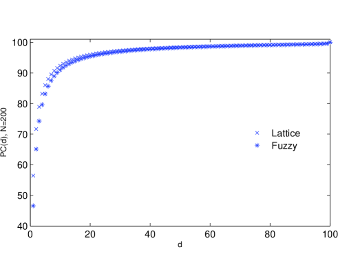
Figure 1: The percentage contributions to the entire entanglement entropy as function of the number of the incorporated DF for the lattice and fuzzy regularization of the sphere.

The operation in question amounts to switching off the entanglement between the DF which are at distance less than $d$-lattice spacing from the separating boundary and the remaining (i.e we include only $d$ DF from the outer and an equal number from the inner region). This is achieved by setting by band to zero all the off-diagonal terms except those corresponding to the $2d+1$ DF to be incorporated .This operation is the same as one of the operations considered in [8, 9].

We compute $S_{N}(d)$ and vary $d$, including successively more distant DF until all DF are included. Each time we compute the percentage contribution to the entropy as a function of $d$

$$PC(d)=100\times S_{N}(d)/S_{N}$$ (2.27)

The results for both models, the fuzzy and lattice regularization, are depicted in Figure 1.

The first thing to note is that, except for the first few DF, the relevance of DF far from the horizon for fuzzy sphere is exactly the same as that in the lattice regularization, the non-commutativity and non-locality have not brought anything new to this point. When only the first few DF are included the lattice and fuzzy regularization have slightly different responses. For the lattice regularization $56\%$ and $71\%$ of the entire entropy is recovered at $d=1$ and $2$ respectively, whereas for the fuzzy sphere we only reach $46\%$ and $65\%$. At $d=10$ we recover $92\%$ in both the fuzzy and the lattice case. For $d>10$ the two curves almost fit together. This similarity between the lattice and the fuzzy regularization regarding the DF dominating the entropy confirms and sharpens the heuristic argument given in [7] to define the boundary in fuzzy sphere case.

Now, the important question to ask here is whether in the macroscopic limit the entropy will captured by the DF infinitesimally close to the boundary. Indeed it is hard to settle this question by numerical methods, one needs an analytical estimation for the contributions of the DF residing at distances which remain finite in the macroscopic limit. Nevertheless, our numerical results suggest strongly that in the macroscopic limit the entropy is given by the contributions of the DF which become infinitesimally close to the boundary. For example for $l=2000$ we find that essentially more than $99\%$ is stored at distance less than $d=150$.

In the last section we will reconsider this point from analytical point of view and give further numerical and qualitative evidences for this.

Before moving to other models there is a technical point that needs to be mentioned here. Although performing the previous operation in the lattice regularization case is straight forward, because the matrices $V^{(m)}$ in such case all have equal dimensions (equal number of DF), for the fuzzy case different sectors corresponding to different $|m|$ have different numbers of DF. For a given $d$, sectors with $N-|m|<d$ already exhaust their maximal contribution, however, we shall show later that in the macroscopic limit these sectors give a negligible contribution to the entropy.

3 Fuzzy Disc and Moyal Plan

Let us now consider the fuzzy disc model and perform the same operations.

The model in question is defined as follow.Consider a scalar theory on ${R}{\times}{R}_{\theta}^{2}$ where ${R}_{\theta}^{2}$ is now the Moyal plane. The action is given by :

$$S=\frac{1}{2}\int dtTr(\dot{\phi}^{2}-\phi\big{(}\nabla^{2}+{\mu}^{2})\phi).$$ (3.1)

The trace is infinite dimensional and the Laplacian is given in terms of creation and annihilation operators $a$ and $a^{+}$ by the expression

$$\nabla^{2}\phi:=-\frac{4}{\theta^{2}}[a^{+},[a,\phi]]=-\frac{4}{\theta^{2}}[a,[a^{+},\phi]].$$ (3.2)

Let us recall that $[a,a^{+}]={\theta}$, where $\theta$ is the noncommutativity parameter. The fuzzy disc is obtained from the plane following [10] as follows. We consider finite dimensional $N{\times}N$ matrices ${\phi}$, viz

$$\phi=\sum_{n,m=0}^{N-1}\phi_{mn}\mid m><n\mid\leavevmode\nobreak\ ,\leavevmode\nobreak\ {\phi}^{+}={\phi}\leavevmode\nobreak\ ,\leavevmode\nobreak\ {\phi}_{nm}^{*}={\phi}_{mn}.$$ (3.3)

Then it can be shown that the Laplacian $\nabla^{2}$ acts on a finite dimensional space of dimension $(N+1)^{2}$, i.e $\nabla^{2}\phi$ is an $(N+1){\times}(N+1)$ matrix. The action on ${\bf R}{\times}{\bf D}_{N}^{2}$ is thus given by (3.1) where the trace $Tr$ is simply cut-off at $N$. We denote this trace by $Tr_{N}$. The radius of the disc is given by

$$R^{2}=N{\theta}.$$ (3.4)

By introducing new variables similar to the ones introduced in the fuzzy sphere case one obtains the following Hamiltonian

$$H=\sum_{m=-(N-1)}^{N-1}H_{m}=\sum_{m=-(N-1)}^{N-1}\sum_{a,b=1}^{N-|m|}\bigg{[}\frac{1}{2}(\pi^{(m)}_{a})^{2}+\frac{1}{2}VQ^{(m)}_{a}Q^{(m)}_{b}\bigg{]}.$$ (3.5)

where $V_{ab}^{(m)}$ is now given by

$$V_{ab}^{(m)} = 2\bigg{[}\big{(}2a+|m|-1+\frac{{\mu}^{2}{\theta}}{4}\big{)}{\delta}_{a,b}-\sqrt{(a-1)(a-1+|m|)}{\delta}_{a-1,b}-\sqrt{a(a+|m|)}{\delta}_{a+1,b}\bigg{]}.$$

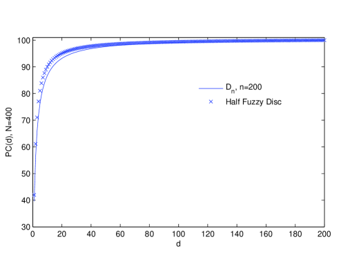
Figure 2: The percentage contributions to the entire entanglement entropy as function of the number of the incorporated DF for the two fuzzy disc cases.

In the fuzzy disc model it turns out that there are two interesting cases to consider for the entanglement entropy. The first one results from tracing out the DF residing inside a smaller subdisc $D_{n}\subset D_{N}$; the second one is to trace half of the fuzzy disc. The tow cases have different behavior if we consider the Moyal plan limit. Whereas in the first case the smaller disc will remain intact and finite when $N$ is sent to infinity, in the second case the ignored region blows up in the Moyal plan limit.

The entanglement entropy resulting from tracing out a fuzzy subdisc $D_{n}$ was computed numerically in [7] and shown to be given by

$$S_{N}(n)=S_{0}+2\sum_{m=1}^{n}S_{m}=0.23(2n+1)$$ (3.7)

For the second case where half of fuzzy disc is traced out the entanglement entropy turned out to be

$$S_{N}=S_{0}+2\sum_{m=1}^{N-1}S_{m}=0.34N$$ (3.8)

In both cases the entanglement entropy is proportional to the boundary degrees of freedom and can be as well interpreted as proportional to the area of the separating boundary ( being here the circumference of a circle in the first case and the diameter of the disc in the second one.)

Let us now address the same question we addressed for the fuzzy sphere case and locate the DF which contribute most to the entanglement entropy.

In the first case, where we trace out a subdisc $D_{n}$, we compute the entanglement entropy $S_{N}(n,d)$ obtained by incorporating only DF from the subdisc $D_{n}$ with $d$ lattice spacing from the separating boundary, that is DF residing in $D_{n}-D_{n-d}$, similarly from the outer region we include only DF with $d$ lattice spacing from the boundary, i.e DF in $D_{n+d}-D_{n}$. Then $d$ is run from $1$ to $n$ .

For the second case the same operation is applied, which is very similar to the fuzzy sphere case. The results for both cases are depicted in Figure 2. Again we see that by including the first few degrees of freedom from the boundary $98\%$ from the total entropy is captured. Nevertheless DF far from the boundary have small contribute, this contribution become smaller and smaller as we move further from the boundary, the DF at $d=n$ contribute by less than $10^{-2}\%$.

4 On the Area Law and Near Boundary Approximation

In the previous sections we showed that the vacuum fluctuations in the vicinity of the horizon ( the separating boundary) are responsible for giving the dominant to the entanglement entropy in different fuzzy space models. The questions that we want address in this section concern the area law itself and the validity of the near boundary approximation in the macroscopic limit.

The considerations of the previews sections suggest strongly that the entanglement entropy should be given by the entanglement between the inner and the outer DF residing at distances which become infinitesimally close to the boundary in the macroscopic limit. Therefore we shall start by giving a simple analytical derivation of the area law using $1/N$ like expansion in the case where the DF incorporated are infinitesimally close to the boundary in large $N$ limit.

Consider first the fuzzy sphere model in the limit of very large $l$ or $N$ and $d/l\ll 1$, .

As already mentioned for a fixed $d$ some sectors already exhaust their maximal contribution, hence we shall distinguish two classes of sectors.

The first class corresponds to the sectors with $|m|\geq 2l-2d+rem(m,2)\equiv m_{d}\leavevmode\nobreak\ \leavevmode\nobreak\$. These are the ones which exhaust their maximal contribution to the entropy, therefore their analysis is valid even when the entire number of DF is incorporated.

The second class corresponds to the sectors with $|m|<2l-2d+rem(m,2)$.

Thus the entropy naturally splits into two contributions

$$S_{N}(d)=S_{\prec}+S_{\succ}\;\;,\;\;S_{\prec}=S_{0}+2\sum_{m=1}^{m_{d}-1}S_{m}(d,l)\;\;,\;\;S_{\succ}=\sum_{m=m_{d}}^{2l}S_{m}(d,l)$$ (4.1)

We start by evaluating $S_{\succ}$ and showing that it vanishes in the $l\rightarrow\infty$.

From equation (2.7) it is not difficult to see that for $d/l\ll 1$ the diagonal elements of $V^{(m)}$ dominate over the off-diagonal ones, this allows for a perturbative evaluation of $S_{m}$ . It is found that

$$S_{m}=\frac{\lambda_{m}}{4}(1-\log\lambda_{m}/4)+O(\lambda^{2}),\leavevmode\nobreak\ \leavevmode\nobreak\ \leavevmode\nobreak\ \lambda_{m}=\frac{1-(\frac{m}{2l})^{2}}{1+(\frac{m}{2l})^{2}}<\frac{d^{2}}{4l^{2}}.$$ (4.2)

from which it follows that

$$S_{\succ}<\frac{d^{3}}{4l^{2}}[1-2\log(d/4l)]+O(d^{5}\log(d/l)/l^{4})$$ (4.3)

this shows that $S_{\succ}$ vanishes in the limit $l\rightarrow\infty$ for all $d<l^{2/3-\epsilon},\leavevmode\nobreak\ \leavevmode\nobreak\ \epsilon>0$. It follows that sectors with number of DF less than $l^{2/3-\epsilon}$ are weakly entangled and have vanishing contributions in the limit of large $l$ and therefore irrelevant for the entanglement entropy.

We now turn our attention to $S_{\prec}$.

We start by noting that for $d\ll l$ the relevant submatrices $V_{d}^{(m)}$ of the matrices $V^{(m)}$ are given by

$${V_{d}^{(m)}}_{ab}=(l^{2}+m^{2}/4)\delta_{ab}-\frac{1}{2}(l^{2}-m^{2}/4)[\delta_{a+1,b}+\delta_{a,b+1}]\leavevmode\nobreak\ \leavevmode\nobreak\ ,\leavevmode\nobreak\ \leavevmode\nobreak\ a,b=1\cdot\cdot\cdot,2d+1-rem(m,2)$$ (4.4)

where we have neglected terms of the order of $ld$.

If we scale $V^{(m)}$ by $1/l^{2}$ and note that the eigenvalues of the matrices $\Lambda^{(m)}$ are invariant under overall scaling of the matrices $V_{d}^{(m)}$, we conclude that $S_{m}$ will depend only on the ratio $m^{2}/(4l^{2})\leavevmode\nobreak\ \leavevmode\nobreak\$. This means that in (4.4) we have neglected effectively terms of the order of $d/l$. In effect, as far as the entanglement is concerned the terms which we have neglected in (4.4) are much less relevant than their order of magnitude may suggest. This will shortly be confirmed by numerical results.

Now, in contrast to the previous class of sectors, these sectors are strongly entangled because the off-diagonal terms are generally of the same order of magnitude as the diagonal ones. Thus no perturbative evaluation of $S_{\prec}$ is possible. Nevertheless equations (4.4) and (4.2 ) are enough to establish the area law.

From equations (4.2) and (4.4) we see that the $S_{m}$’s depend exclusively on the ratios $\frac{m}{2l}$ and the entropy is therefore given by

$$S_{N}(d)=S(0,d)+2\sum_{m=1}^{2l}S(m^{2}/4l^{2},d)$$ (4.5)

In the large $l$ limit $S_{N}(d)$ can be well approximated by integral

$$S_{N}(d)=4l\int_{0}^{1}S(x^{2},d)dx$$ (4.6)

Equation (4.6) establishes the area law; and shows that for $l\gg d$ the percentage by which the near boundary DF contribute becomes independent of the size of the boundary in the macroscopic limit. Of course, equation (4.6) is understood to be exactly valid only in the strict limit, otherwise correction terms would be present and which vanish in the macroscopic limit. The above analytical results can be confirmed by several numerical evaluations of $S_{N}(d)$ for fixed $d$ and various values of $N$ or $l$ . For example, if we define $c_{N}(d)=S_{N}(d)/l$ it is found that $c_{1000}(d=20)-c_{1600}(d=20)\sim 10^{-6}$.

Let us now consider the fuzzy disc model. In the case where we trace out a subdisc $D_{n}$ and incorporate only DF from the outer and inner region with $d$ lattice spacing distance from the boundary, we too find that we have to distinguish two classes of sectors.

The first class with $|m|\geq n-d$. In this case we again observe that for $d\ll n$ the diagonal elements dominate over off-diagonal ones and $S_{m}$ can be evaluated perturbatively . We find

$$S_{m}=\frac{\lambda_{m}}{4}(1-\log\lambda_{m}/4)+O(\lambda^{2})\leavevmode\nobreak\ \leavevmode\nobreak\ ,\leavevmode\nobreak\ \leavevmode\nobreak\ \lambda_{m}=\frac{1-|m|/n}{(2-|m|/n)^{2}}$$ (4.7)

and it follows that

$$S_{\succ}<\frac{d^{2}}{8n}(1-\log(d/16n))+O(d^{2}\log(n/d)/n^{2})$$ (4.8)

Again we see that sectors with number of DF negligible compared to $n$ give small and vanishing contributions in the macroscopic limit. However, the rate by which $S_{\succ}$ approaches zero is slower than the fuzzy sphere case.

It should be noted also that, unlike the fuzzy sphere case, not all sectors with $|m|\geq|m|-d$ exhaust their maximal contribution. This is due to the fact that for some sectors certain outer DF are still left out.

Consider now the second class of sectors, namely the ones with $|m|<|m|-d+1$. For $d\ll n$ we find

$${V_{d}^{(m)}}_{ab}=(2n-|m|)\delta_{ab}-\sqrt{n(n-|m|)}[\delta_{a+1,b}+\delta_{a,b+1}]+O(d)$$ (4.9)

Again, we use the fact that $S_{m}$ is invariant under scaling of $V^{(m)}$ and conclude that $S_{m}$ depends only the ratio $|m|/n$ and $d$. Therefore

$$S_{N}(d)=S_{\succ}(|m|/n,d)+S_{\prec}(|m|/n,d)$$ (4.10)

in the large $n$ limit (4.10) can be approximated by and integral, which becomes exact in the limit $n\rightarrow\infty$,

$$S_{N}(d)=2n\int_{0}^{1}S(x,d)dx\leavevmode\nobreak\ \leavevmode\nobreak\$$ (4.11)

This establishes the area law and shows that percentage by which the DF contribute to the entire entropy is independent of $n$ in the macroscopic limit. This result can as well be confirmed by several numerical calculations.

The case when we trace out half of the fuzzy disc is technically similar to the fuzzy sphere, however the asymptotic behaviors are similar to the subdisc case.

Some comments about the above results are in order. We have established that there are generally two classes of sectors. The first class is what we may call the irrelevant sectors or the weakly entangled ones, such sectors have a small number of DF compared to the number of the boundary DF and have vanishing contribution in the macroscopic limit. The second class is made of sectors which have number of DF of the order of the number of boundary DF. These sectors are strongly entangled and give the essential contribution to the entanglement entropy. However, these results go somehow against to what one may have naively guessed. The fact the entropy is proportional to the number of sectors does not mean that all sectors have relatively comparable contributions. Indeed, it is the fact that the eigenvalues of the reduced density operator depend only on the ratios $m^{2}/4l^{2}$ or $|m|/n$ which leads naturally to the area law, and this in turn will be related below to the validity of the near boundary approximation.

It is interesting to mention here that in deriving equations (4.6) and (4.11) we have made no real explicit use of the eigenvalues or $S_{m}$, the area law is almost dictated by the general properties of the entanglement entropy and the form of the fuzzy potentials $V^{(m)}$’s .

Note that quite similar remarks apply to the lattice regularization of the continuum sphere; sectors with $m$ much larger than $N$ have small vanishing contributions [7]. However in the lattice regularization no analytical derivation of the area seems easy to obtain in the limit $d\ll N$.

We end this paper by reconsidering the area law for the entanglement entropy when we include all DF. We shall do this for the fuzzy sphere. Similar arguments hold for the fuzzy disc. The aim is to qualitatively argue that in the limit of large $N$ or $l$ equation (4.6) remains true when we include all DF from the inner and the outer region, that is $S_{m}$ will be functions of $m^{2}/4l^{2}$ only .

We start by noting that the approximation given in equation (4.4) remains valid for all DF at $d$-lattice distance from the boundary as long as $d/l\rightarrow 0$ in the macroscopic limit. Also, it is easy to see that the same approximation is valid for the weakly entangled sectors. Now, for the remaining DF from the strongly entangled sectors one has to distinguish tow classes of DF. The ones at $d$ such that $(l-m/2-d)/l\ll 1$, these DF are the ones that are far away from the boundary, and the ones for which $d$ is of the order of $l$, these are at an intermediate distances. For the first class it is not difficult to show that their corresponding off-diagonal elements die-off like $1/l$ and therefore they disentangle from the other DF and become irrelevant in the macroscopic limit. For the second class none of the above approximations is valid. However our numerical calculations show that those DF are as well irrelevant. A quantitative argument for this can be given as follows.

Let $\lambda$ be one of the eigenvalues of a given $\Lambda^{(m)}$, equation (2.25). Any eigenvalue will be a function of the off-diagonal elements of the matrix $V^{(m)}$ , $(v_{12},v_{23},\cdot\cdot\cdot v_{k,k+1},\cdot\cdot\cdot v_{n-1,n})$, where $v_{k,k+1}$ is the boundary element which couples the inner DF to the outer ones. First, it is by default that all the eigenvalues vanish identically if $v_{k,k+1}$ is set to zero. Also, the eigenvalues are all decreasing functions of the off-diagonal terms. On the other hand, setting one of the off-diagonal elements at position $d$ to zero would kill the contributions of all the successors with positions $p>d$. This leads to the conclusion that the contribution of DF at position $d$ should be a decreasing function of the product $\prod_{i<d}v_{k+i,k+i+1}$, hence the contribution of this DF will be suppressed in view of the fact that the elements $v_{i,i+1}$ are all less than $1/2$. Indeed if we assume the existence of a Taylor expansion for the eigenvalues in terms of the off-diagonal elements, it is easy to see that every term in the expansion which contains some power of an off-diagonal element located at position $d$ must be accompanied by some power of all the precedent off-diagonal elements.

The above argument is of course only suggestive. Indeed it would be interesting to obtain an asymptotic estimation of the contribution of a DF at distance of the order of $l$.

Now, as an evidence for the above arguments let us push the near boundary (horizon) approximation far beyond its region of validity and assume it to be valid everywhere and compute the resulting entanglement entropy including all DF. That is, we take our starting potentials the ones given by (4.4) instead of the ones given by (2.7),

$${V^{(m)}}_{ab}=(l^{2}+m^{2}/4)\delta_{ab}-\frac{1}{2}(l^{2}-m^{2}/4)[\delta_{a+1,b}+\delta_{a,b+1}]\leavevmode\nobreak\ \leavevmode\nobreak\ ,\leavevmode\nobreak\ \leavevmode\nobreak\ a,b=1,\cdot\cdot\cdot 2l+1-m,$$ (4.12)

compute the entanglement entropy incorporating all DF and compare it to the one obtained using the exact form of $V^{(m)}$ of equation (2.7). Note first that the area law follows automatically from (4.12), as all eigenvalues are functions only of $m^{2}/4l^{2}$ (after scaling all matrices by $1/l^{2}$).

Table 1 shows the values of the scaled entropy $S_{N}/l$ obtained using the extended near boundary approximation of the potentials against the values obtained by the original (exact) ones. According to these numerical results the near boundary approximation capture almost the exact value and become more accurate as $l$ is pushed towards larger values, the deviation from the exact true value is of the order of $1/l$. In the macroscopic limit we would expect to obtain an exact agreement.

Indeed, it is not difficult to see why using the near boundary approximation every where gives the same result in the large $l$ limit. First, the near boundary approximation capture the true contribution of all near boundary DF and is valid for the weakly entangled sectors. For the DF far from the boundary, the potentials given by (4.12) provide essentially the same order of suppression for their contributions as the exact potentials do.

$l$	200	300	500	600	900
Exact form	0.3960	0.3960	0.3960	0.3960	0.3960
Near boundary approximation	0.3929	0.3939	0.3948	0.3950	0.3953

The validity of the near boundary approximation shows that for the entanglement entropy all that matters is the near boundary ( horizon) geometry. This result goes in agreement with the standard results and paradigm about black hole thermodynamics and field theories in the presence of black hole [4, 6, 11]. Finally, it is interesting to note that despite the non-locality and UV-IR mixing phenomena on fuzzy and non-commutative spaces, entanglement entropy is still controlled by the near boundary geometry.

Acknowledgements

The author would like to thank E.I Lashin for useful discussions. This work is supported by King Saud University, College of Science-Research Center Project No: (phys/2008/34).

References

- [1] L.Bombelli, R.K.Koul, J.Lee, and R.Sorkin, Phys.Rev. D34,373 (1986).
- [2] M.Srednicki, Phys.Rev.Lett 71 666 (1993)
- [3] C.Callan and F.Wilczek, Phys.Lett. B333 55-61 (1994), [arXiv:hep-th/9401072].
- [4] L.Susskind and J.Uglum, D50 2700-2711 (1994) , [arXiv:hep-th/9401070].
- [5] R. Sorkin, Stud.Hist. Philos.Mod.Phys. 26, 291 (2005).
- [6] Daniela Bigatti, Leonard Susskind, TASI lectures on the Holographic Principle, [hep-th/0002044]
- [7] Dou D, B Ydri, Phys.Rev D 74, (2006) 044014, [gr-qc/0605003].
- [8] S.Das,S. Shankaranarayanan, Class.Quant.Grav 24 5299-5306,(2007), [gr-qc/0703082].
- [9] S. Das, S. Shankaranarayanan, S.Sur, Can.J.Phys 86,653-658, (2008), [gr-qc/07102013].
- [10] F. Lizzi, P. Vitale, A. Zampini, JHEP 0308 (2003) 057,[arXiv:hep-th/0306247] .
- [11] A.Strominger, JHEP 9802 (1998) 009,[arXiv:hep-th/9712251]