Theory of angular Goos-Hänchen shift near Brewster incidence

Abstract

We present here a compactly formulated application of the previously posted general formalism of the reflection of Gaussian beams at a dielectric interface (arXiv:0710.1643v2 [physics.optics]). Specifically, we calculate the Goos-Hänchen shift near Brewster incidence, for an air-glass plane interface.

I Introduction

When a beam of light impinges upon a plane interface separating two transparent media, it produces reflected and transmitted beams. In 1815 the Scottish physicist David Brewster discovered the total polarization of the reflected beam at the angle $\theta_{B}$ since named after him Brewster (1815). From his observations he was also able to empirically determine the celebrated equation, known as Brewster’s law, $\tan\theta_{B}=n_{1}/n_{2}$, where $n_{1}$ and $n_{2}$ are the respective refractive indices of the two media.

In this work we calculate the Goos-Hänchen shift occurring near Brewster incidence at an air-glass plane interface, for an incident Gaussian beam.

II Theory

Consider a monochromatic beam of light incident upon a plane interface that separates two homogeneous and isotropic media. The first medium, say air, has refractive index $n_{<}$ and the second medium, say glass, has refractive index $n_{>}$. With $n=\frac{n_{>}}{n_{<}}$ we denote the ratio between the two refractive indices. Here $n$ can be either a real or a complex number, in the latter case at least one of the two media exhibits absorption. Without lack of generality, we assume that the beam meets the interface coming from the air side. Thus, it will be convenient to take the axis $z$ of the laboratory Cartesian frame $K=(O,x,y,z)$ normal to the interface and directed from the air to the glass. Moreover, we choose the origin $O$ in a manner that the plane interface has equation $z=0$. The air-glass interface, the incident and the reflected beams are pictorially illustrated in Fig. 1.

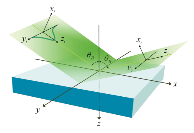
Figure 1: (Color online) Geometry of beam reflection at the air-medium interface. $\theta_{B}$ is the Brewster angle.

In addition to the laboratory frame, we use a Cartesian frame $K_{i}=(O,x_{i},y_{i},z_{i})$ attached to the incident beam and another one $K_{r}=(O,x_{r},y_{r},z_{r})$ attached to the reflected beam. Let $\mathbf{k}_{0}=k_{0}\hat{\mathbf{z}}_{i}$ and $\mathbf{k}$ denote the central and noncentral wave vectors of the incident beam, respectively, with $\lvert\mathbf{k}\rvert=\lvert\mathbf{k}_{0}\rvert=k_{0}$. We choose the laboratory frame $K$ in such a way that $\hat{\mathbf{z}}_{i}=\hat{\mathbf{x}}\sin\theta+\hat{\mathbf{z}}\cos\theta$. In this manuscript with either $\hat{\mathbf{u}}$ or $\hat{\mathbf{u}}_{\,a}$ we denote a real unit vector directed along the Cartesian frame axis $u$, where $u\in\{x,y,z\}$, and $a\in\{i,r\}$.

The electric field of the incident beam at the air side of the interface $(z<0)$, can be written in the angular spectrum representation Mandel and Wolf (1995) as

$$\mathbf{E}^{I}(\mathbf{r}) =\sum_{\lambda=1}^{2}\iint\limits_{-\infty}^{\hphantom{xxii}\infty}\hat{\mathbf{e}}_{\lambda}(U,V,\theta)E_{\lambda}(U,V)e^{i\left(UX_{i}+VY_{i}+WZ_{i}\right)}\;\mathrm{d}U\,\mathrm{d}V,$$ (1)

where $U=\mathbf{k}\cdot\hat{\mathbf{x}}_{i}/k_{0}$, $V=\mathbf{k}\cdot\hat{\mathbf{y}}_{i}/k_{0}$, and $W=(1-U^{2}-V^{2})^{1/2}$. Moreover, we have defined $X_{a}=k_{0}x_{a}$, $Y_{a}=k_{0}z_{a}$, $Z_{a}=k_{0}z_{a}$, with $a\in\{i,r\}$, and $\mathbf{r}$ so . The polarization unit basis vectors $\{\hat{\mathbf{e}}_{\lambda}\}_{\lambda\in\{1,2\}}$ have been chosen as

$$\hat{\mathbf{e}}_{1}=\frac{\hat{\mathbf{e}}_{2}\times{\mathbf{k}}}{\lvert\hat{\mathbf{e}}_{2}\times{\mathbf{k}}\rvert},\qquad\hat{\mathbf{e}}_{2}=\frac{\hat{\mathbf{z}}\times{\mathbf{k}}}{\lvert\hat{\mathbf{z}}\times{\mathbf{k}}\rvert},$$ (2)

where the symbol “$\times$” denotes the standard vector product in $\mathbb{R}^{3}$. Here $\hat{\mathbf{z}}$ is a real unit vector directed along the laboratory axis $z$ and, by definition,

$${\mathbf{k}} =k_{0}\left(U\hat{\mathbf{x}}_{i}+V\hat{\mathbf{y}}_{i}+W\hat{\mathbf{z}}_{i}\right)$$

$$=\hat{\mathbf{x}}k_{x}+\hat{\mathbf{y}}{k_{y}}+\hat{\mathbf{z}}\sqrt{k_{0}^{2}-k_{x}^{2}-k_{y}^{2}}.$$ (3)

By substituting Eq. (3) into Eq. (2) we obtain

$$\hat{\mathbf{e}}_{1}(U,V,\theta) =\frac{\left[UWc+\left(W^{2}+V^{2}\right)s\right]\hat{\mathbf{x}}_{i}+V\left(Wc-Us\right)\,\hat{\mathbf{y}}_{i}-\left[\left(U^{2}+V^{2}\right)c+UWs\right]\,\hat{\mathbf{z}}_{i}}{\left[V^{2}+\left(Uc+Ws\right)^{2}\right]^{1/2}},$$ (4)

$$\hat{\mathbf{e}}_{2}(U,V,\theta) =\frac{-{Vc}\,\hat{\mathbf{x}}_{i}+\left(Uc+Ws\right)\,\hat{\mathbf{y}}_{i}-Vs\,\hat{\mathbf{z}}_{i}}{\left[V^{2}+\left(Uc+Ws\right)^{2}\right]^{1/2}},$$ (5)

where we used the shorthand $c=\cos\theta$ and $s=\sin\theta$, and $\theta$ is the central angle of incidence defined as: $\theta=\arccos(\hat{\mathbf{z}}_{i}\cdot\hat{\mathbf{z}})$. For well collimated paraxial beams ($U^{2}+V^{2}\ll 1$) the expressions above reduce to

$$\hat{\mathbf{e}}_{1} \simeq{\hat{\mathbf{x}}_{i}+\hat{\mathbf{y}}_{i}\,V\cot\theta-\hat{\mathbf{z}}_{i}\,U},$$ (6)

$$\hat{\mathbf{e}}_{2} \simeq{-\hat{\mathbf{x}}_{i}\,V\cot\theta+\hat{\mathbf{y}}_{i}-\hat{\mathbf{z}}_{i}\,V},$$ (7)

$$\hat{\mathbf{e}}_{3} \simeq{\hat{\mathbf{x}}_{i}\,U+\hat{\mathbf{y}}_{i}V+\hat{\mathbf{z}}_{i}},$$ (8)

where $\hat{\mathbf{e}}_{3}\equiv\mathbf{k}/k_{0}\equiv\hat{\mathbf{k}}$. From Eq. (2) it follows that $\hat{\mathbf{e}}_{1}$ lies in the plane containing both the wave vector $\mathbf{k}$ and $\hat{\mathbf{z}}$, usually denoted as the plane of incidence with respect to $\mathbf{k}$, while $\hat{\mathbf{e}}_{2}$ is orthogonal to such a plane. Both $\hat{\mathbf{e}}_{1}$ and $\hat{\mathbf{e}}_{2}$ are orthogonal to $\mathbf{k}$ by definition, and $\{\hat{\mathbf{e}}_{1},\hat{\mathbf{e}}_{2},\hat{\mathbf{k}}\}$ form a complete, orthogonal basis in $\mathbb{R}^{3}$. Conventionally, a plane wave whose electric field is parallel to either $\hat{\mathbf{e}}_{1}$ or $\hat{\mathbf{e}}_{2}$, is referred to as either a TM or a TE wave, respectively. The symbols P for TM and S for TE, are also widely used. In Eq. (1) the functions $E_{\lambda}(U,V)$ determine the shape and the polarization of the beam. These amplitudes are always expressible as $E_{\lambda}(U,V)=A(U,V)\,\alpha_{\lambda}(U,V)$, where $A(U,V)$ and $\alpha_{\lambda}(U,V)$ are the scalar and the vector spectral amplitudes of the field, respectively. The first determines the spatial characteristics of the beam, while the second sets the polarization of the beam Aiello and Woerdman (2008). Here we consider a collimated, monochromatic beam, with a Gaussian spectral amplitude

$$A(U,V)=\exp\left(-\frac{U^{2}+V^{2}}{\theta_{0}^{2}}\right)\exp\left(iWD\right),$$ (9)

where $\theta_{0}=2/(k_{0}w_{0})$ is the angular spread of the incident beam with a minimum spot size (waist) $w_{0}$ located at $Z_{i}=-D$ Mandel and Wolf (1995). In order to determine the vector spectral amplitudes $\alpha_{\lambda}(U,V)$ of the incident beam, we assume that the beam has passed across a polarizer plate perpendicular to the central wave vector $k_{0}\hat{\mathbf{z}}_{i}$ of the beam. Let $\hat{\mathbf{f}}=f_{P}\hat{\mathbf{x}}_{i}+f_{S}\hat{\mathbf{y}}_{i}$ denotes a complex-valued unit vector that represents the orientation of the polarizer, with $\lvert f_{P}\rvert^{2}+\lvert f_{P}\rvert^{2}=1$. Then, we determine the amplitudes $\alpha_{\lambda}(U,V)$ by imposing

$$\sum_{\lambda=1}^{2}\hat{\mathbf{e}}_{\lambda}(U,V,\theta)\alpha_{\lambda}(U,V)=\hat{\mathbf{f}}-\hat{\mathbf{k}}\bigl{(}\hat{\mathbf{k}}\cdot\hat{\mathbf{f}}\bigr{)},$$ (10)

where we used the polarizer representation given in Ref. Fainman and Shamir (1984). Since the completeness of the basis $\{\hat{\mathbf{e}}_{1},\hat{\mathbf{e}}_{2},\hat{\mathbf{k}}\}$ implies, for any vector $\mathbf{v}$, the validity of the following relation

$$\hat{\mathbf{e}}_{1}(\hat{\mathbf{e}}_{1}\cdot\mathbf{v})+\hat{\mathbf{e}}_{2}(\hat{\mathbf{e}}_{2}\cdot\mathbf{v})=\mathbf{v}-\hat{\mathbf{k}}(\hat{\mathbf{k}}\cdot\mathbf{v}),$$ (11)

then from Eq. (10) it immediately follows that

$$\alpha_{\lambda}(U,V)=\hat{\mathbf{e}}_{\lambda}(U,V,\theta)\cdot\hat{\mathbf{f}}.$$ (12)

Thus, from Eqs. (4-5) and (12) we obtain

$$\alpha_{1}(U,V) =\frac{W\left(Uf_{P}+Vf_{S}\right)\cos\theta-\left[UVf_{S}-\left(W^{2}+V^{2}\right)f_{P}\right]\sin\theta}{\left[V^{2}+\left(U\cos\theta+W\sin\theta\right)^{2}\right]^{1/2}},$$ (13)

$$\alpha_{2}(U,V) =\frac{\left(Uf_{S}-Vf_{P}\right)\cos\theta+Wf_{S}\sin\theta}{\left[V^{2}+\left(U\cos\theta+W\sin\theta\right)^{2}\right]^{1/2}},$$ (14)

that reduce, for paraxial beams, to

$$\alpha_{1}(U,V) \simeq f_{P}+f_{S}V\cot\theta,$$ (15)

$$\alpha_{2}(U,V) \simeq f_{S}-f_{P}V\cot\theta.$$ (16)

When the beam is reflected at the interface, each plane wave mode function

$$\hat{\mathbf{e}}_{\lambda}(U,V,\theta)e^{i\left(UX_{i}+VY_{i}+WZ_{i}\right)}=\hat{\mathbf{e}}_{\lambda}(\mathbf{k})e^{i\mathbf{k}\cdot\mathbf{r}},$$ (17)

changes according to

$$\hat{\mathbf{e}}_{\lambda}(\mathbf{k})e^{i\mathbf{k}\cdot\mathbf{r}}\mapsto r_{\lambda}(\mathbf{k})\hat{\mathbf{e}}_{\lambda}(\widetilde{\mathbf{k}})e^{i\widetilde{\mathbf{k}}\cdot\mathbf{r}},$$ (18)

where $r_{1}(\mathbf{k})$ and $r_{2}(\mathbf{k})$ are the Fresnel reflection amplitudes for TM and TE waves, respectively Born and Wolf (2003),

$$r_{1}(\mathbf{k})=\displaystyle{\frac{n^{2}k_{z}-k_{z}^{t}}{n^{2}k_{z}+k_{z}^{t}}},\qquad\qquad r_{2}(\mathbf{k})=\displaystyle{\frac{k_{z}-k_{z}^{t}}{k_{z}+k_{z}^{t}}},$$ (19)

and $\widetilde{\mathbf{k}}=\mathbf{k}-2\,\hat{\mathbf{z}}\left(\hat{\mathbf{z}}\cdot\mathbf{k}\right)$ is set by the law of specular reflection Gragg (1988), while the unit vectors $\hat{\mathbf{e}}_{\lambda}(\widetilde{\mathbf{k}})$ are defined as in Eq. (2) with $\mathbf{k}\mapsto\widetilde{\mathbf{k}}$. In Eqs. (19) $k_{z}^{t}$ is the $z$-component of the wave vector inside the glass, namely

$$k_{z}^{t}=\left(n^{2}k_{0}^{2}-k_{x}^{2}-k_{y}^{2}\right)^{1/2}.$$ (20)

It is worth noting that here $k_{x},k_{y},k_{z}$ are the Cartesian components of the wave vector $\mathbf{k}$ with respect to the laboratory frame $K$, while in Eq. (1) the integrations are performed with respect to the variables $U$ and $V$ which are the transverse Cartesian components of the wave vector $\mathbf{k}$ with respect to the incident-beam frame $K_{i}$. Therefore, it will be useful to express $r_{1}(\mathbf{k})$ and $r_{2}(\mathbf{k})$ in terms of $U$ and $V$. From Eq. (3) it straightforwardly follows that

$$r_{1}(U,V) =\,\frac{n^{2}\left(W\cos\theta-U\sin\theta\right)-\left[n^{2}-V^{2}-\left(W\sin\theta+U\cos\theta\right)^{2}\right]^{1/2}}{n^{2}\left(W\cos\theta-U\sin\theta\right)+\left[n^{2}-V^{2}-\left(W\sin\theta+U\cos\theta\right)^{2}\right]^{1/2}},$$ (21)

$$r_{2}(U,V) =\,\frac{W\cos\theta-U\sin\theta-\left[n^{2}-V^{2}-\left(W\sin\theta+U\cos\theta\right)^{2}\right]^{1/2}}{W\cos\theta-U\sin\theta+\left[n^{2}-V^{2}-\left(W\sin\theta+U\cos\theta\right)^{2}\right]^{1/2}}.$$ (22)

It is easy to check that $r_{1}(U,V)$ and $r_{2}(U,V)$ reduce to the ordinary Fresnel coefficients for $U=0$ and $V=0$:

$$r_{1}^{0}(\theta)\equiv r_{1}(0,0) =\,\frac{n^{2}\cos\theta-\left(n^{2}-\sin^{2}\theta\right)^{1/2}}{n^{2}\cos\theta+\left(n^{2}-\sin^{2}\theta\right)^{1/2}},$$ (23)

$$r_{2}^{0}(\theta)\equiv r_{2}(0,0) =\,\frac{\cos\theta-\left(n^{2}-\sin^{2}\theta\right)^{1/2}}{\cos\theta+\left(n^{2}-\sin^{2}\theta\right)^{1/2}}.$$ (24)

In the remaining of this manuscript, we shall often benefit from the following relations satisfied by the reflection coefficients defined above:

$$\left.\frac{\partial\,r_{\lambda}}{\partial U}\right|_{U=0,\,V=0} =\frac{\partial\,r_{\lambda}^{0}}{\partial\theta},\qquad\left.\frac{\partial\,r_{\lambda}}{\partial V}\right|_{U=0,\,V=0}=0,$$ (25)

and

$$\left.\frac{\partial^{\,2}\,r_{\lambda}}{\partial U^{2}}\right|_{U=0,\,V=0} =\frac{\partial^{2}\,r_{\lambda}^{0}}{\partial\theta^{2}},\qquad\left.\frac{\partial^{\,2}\,r_{\lambda}}{\partial V^{2}}\right|_{U=0,\,V=0}=\cot\theta\frac{\partial\,r_{\lambda}^{0}}{\partial\theta},\qquad\left.\frac{\partial^{\,2}\,r_{\lambda}}{\partial U\partial V}\right|_{U=0,\,V=0}=0,$$ (26)

where $\lambda\in\{1,2\}$.

From Eq. (18) it follows that, after reflection, the electric field of the beam can be written as

$$\mathbf{E}^{I}(\mathbf{r})\mapsto\mathbf{E}^{R}(\mathbf{r}) =\sum_{\lambda=1}^{2}\iint\limits_{-\infty}^{\hphantom{xxii}\infty}\hat{\mathbf{e}}_{\lambda}(\widetilde{\mathbf{k}})r_{\lambda}(U,V)E_{\lambda}(U,V)e^{i\left(-UX_{r}+VY_{r}+WZ_{r}\right)}\;\mathrm{d}U\,\mathrm{d}V,$$ (27)

where $\hat{\mathbf{e}}_{\lambda}(\widetilde{\mathbf{k}})=\hat{\mathbf{e}}_{\lambda}(-U,V,\pi-\theta)$, namely:

$$\hat{\mathbf{e}}_{1}(\widetilde{\mathbf{k}}) =\frac{\left[UWc+\left(W^{2}+V^{2}\right)s\right]\hat{\mathbf{x}}_{r}-V\left(Wc-Us\right)\,\hat{\mathbf{y}}_{r}+\left[\left(U^{2}+V^{2}\right)c+UWs\right]\,\hat{\mathbf{z}}_{r}}{\left[V^{2}+\left(Uc+Ws\right)^{2}\right]^{1/2}},$$ (28)

$$\hat{\mathbf{e}}_{2}(\widetilde{\mathbf{k}}) =\frac{{Vc}\,\hat{\mathbf{x}}_{r}+\left(Uc+Ws\right)\,\hat{\mathbf{y}}_{r}-Vs\,\hat{\mathbf{z}}_{r}}{\left[V^{2}+\left(Uc+Ws\right)^{2}\right]^{1/2}},$$ (29)

where we used again the shorthand $c=\cos\theta$ and $s=\sin\theta$. In Eq. (27) we have exploited the fact that by definition

$$\widetilde{\mathbf{k}}\cdot\mathbf{r}=k_{x}x+k_{y}y-k_{z}z=-UX_{r}+VY_{r}+WZ_{r},$$ (30)

where the latter equality is written in terms of the Cartesian coordinates of the position vector $\mathbf{r}$ with respect to the reflected beam reference frame $K_{r}$.

If the air-glass interface would behave as and ideal reflecting surface characterized by wave vector-independent reflection amplitudes $r_{1}(\mathbf{k})=1$ and $r_{2}(\mathbf{k})=-1$, then the reflected beam were just the mirror-image of the incident one Aie . However, in the real world, as a result of the polarization and wave vector dependence of the Fresnel amplitudes $r_{\lambda}(\mathbf{k})$, non-specular reflection phenomena occur, the most prominent of which are the so-called Goos-Hänchen (GH) Goos and Hanchen (1947) and Imbert-Fedorov (IF) de Beauregard and Imbert (1972) shifts that amount, respectively, to a longitudinal and a transverse displacement of the reflected beam with respect to the mirror-image of the incident one. Such displacements can be assessed by measuring the position of the center of the reflected beam with a quadrant detector centered at $x_{r}=0,\,y_{r}=0$ along the reference axis $z_{r}$ attached to the reflected central wave vector $\widetilde{\mathbf{k}}_{0}=k_{0}\hat{\mathbf{z}}_{r}$. A quadrant detector has four sensitive areas each delivering a photocurrent when illuminated. The difference between these photocurrents is proportional to the displacement of the barycenter of the beam intensity $I(X_{r},Y_{r},Z_{r})$ relative to center of the detector. In other words, this displacement is proportional to the first order moments $\langle\mathbf{X}\rangle=\langle X_{r}\rangle\hat{\mathbf{x}}_{r}+\langle Y_{r}\rangle\hat{\mathbf{y}}_{r}$ of the intensity distribution function of the beam Porras (1997):

$$\langle\mathbf{X}\rangle=\frac{\displaystyle{\iint\limits_{-\infty}^{\hphantom{xxii}\infty}}\mathbf{X}\,I(X_{r},Y_{r},Z_{r})\text{d}X_{r}\text{d}Y_{r}}{\displaystyle{\iint\limits_{-\infty}^{\hphantom{xxii}\infty}I(X_{r},Y_{r},Z_{r})\text{d}X_{r}\text{d}Y_{r}}}.$$ (31)

In order to evaluate $\langle\mathbf{X}\rangle$ we need to know the intensity $I(X_{r},Y_{r},Z_{r})$ that, apart from an irrelevant proportionality factor, can be defined as

$$I(X_{r},Y_{r},Z_{r})\equiv\lvert\mathbf{E}^{R}(X_{r},Y_{r},Z_{r})\rvert^{2}.$$ (32)

Thus, we must calculate the double integral in Eq. (27). To this end, we exploit the fact that for a well collimated beam $\theta_{0}\ll 1$, and that Eq. (9) implies that $A(U,V)\simeq 0$ outside the paraxial domain $\mathcal{P}=\{U,V:U^{2}+V^{2}\ll 1\}$. In this domain

$$W=\left(1-U^{2}-V^{2}\right)^{1/2}\simeq 1-\frac{U^{2}+V^{2}}{2},$$ (33)

and we can rewrite Eq. (27) as

$$\mathbf{E}^{R}(\mathbf{r}) =e^{i(Z_{r}+D)}\iint\limits_{-\infty}^{\hphantom{xxii}\infty}\bm{\mathcal{E}}(U,V)e^{-\frac{U^{2}+V^{2}}{2}\left[\Lambda+i(Z_{r}+D)\right]}e^{i\left(-UX_{r}+VY_{r}\right)}\;\mathrm{d}U\,\mathrm{d}V,$$ (34)

where we have defined $\Lambda=2/\theta_{0}^{2}=k_{0}L$, with $L$ equal to the Raleigh range of the beam Mandel and Wolf (1995). Equation (34) is still exact, and it defines $\bm{\mathcal{E}}(U,V)$ as

$$\bm{\mathcal{E}}(U,V) =\displaystyle{\sum_{\lambda=1}^{2}\hat{\mathbf{e}}_{\lambda}(\widetilde{\mathbf{k}})r_{\lambda}(U,V)\alpha_{\lambda}(U,V)e^{i(Z_{r}+D)\left[W-\left(1-\frac{U^{2}+V^{2}}{2}\right)\right]}},$$ (35)

which can be evaluated within the paraxial domain $\mathcal{P}$ via a Taylor expansion of the form

$$\bm{\mathcal{E}}(U,V) \simeq\bm{\mathcal{E}}(0,0)+\left(U\bm{\mathcal{E}}_{U}+V\bm{\mathcal{E}}_{V}\right)+\frac{1}{2}\left(U^{2}\bm{\mathcal{E}}_{UU}+2UV\bm{\mathcal{E}}_{UV}+V^{2}\bm{\mathcal{E}}_{VV}\right)+\ldots,$$ (36)

where we used the obvious notation $\bm{\mathcal{E}}_{U}=\left.\partial\bm{\mathcal{E}}(U,V)/\partial U\right|_{U=0,V=0}$, and so on. Usually, to calculate both GH and IF shifts, first order Taylor expansions is enough. However, as we shall see soon, at Brewster incidence it becomes necessary to keep second order terms to avoid divergences in the expressions of the shifts. Substitution of Eq. (36) in Eq. (34) permits the analytical evaluation of the Gaussian integrals; this leads to the following expression for the electric field of the reflected beam:

$$\mathbf{E}^{R}(\mathbf{r}) \simeq\psi(\mathbf{r})\bigl{(}\hat{\mathbf{x}}_{r}E_{x_{r}}^{R}+\hat{\mathbf{y}}_{r}E_{y_{r}}^{R}+\hat{\mathbf{z}}_{r}E_{z_{r}}^{R}\bigr{)},$$ (37)

where

$$\psi(\mathbf{r}) =\frac{1}{\displaystyle{Z-i\Lambda}}\exp\left({\frac{\displaystyle{i}}{\displaystyle{2}}\frac{\displaystyle{X^{2}+Y^{2}}}{\displaystyle{Z-i\Lambda}}}\right),$$ (38)

is the scalar amplitude of a fundamental Gaussian beam, and

$$E_{x_{r}}^{R}= \,f_{P}r_{P}+f_{S}\frac{Y\left(r_{P}+r_{S}\right)\cot\theta}{Z-i\Lambda}-f_{P}\frac{Xr_{P}^{\prime}}{Z-i\Lambda}$$

$$\,+f_{P}\frac{X^{2}\left(r_{P}^{\prime\prime}-2r_{P}\right)}{2(Z-i\Lambda)^{2}}+f_{P}\frac{Y^{2}\left[r_{P}^{\prime}-2\left(r_{P}+r_{S}\right)\cot\theta\right]\cot\theta}{2(Z-i\Lambda)^{2}}$$

$$\,-if_{P}\frac{r_{P}^{\prime\prime}+2r_{S}-2\left(r_{P}+r_{S}\right)\csc^{2}\theta+r_{P}^{\prime}\cot\theta}{2(Z-i\Lambda)}$$

$$\,+f_{S}\frac{XY\left[2r_{P}+r_{S}+r_{S}\cos(2\theta)-\left(r_{P}^{\prime}+r_{S}^{\prime}\right)\sin(2\theta)\right]\csc^{2}\theta}{2(Z-i\Lambda)^{2}},$$ (39)

$$E_{y_{r}}^{R}= \,f_{S}r_{S}-f_{P}\frac{Y\left(r_{P}+r_{S}\right)\cot\theta}{Z-i\Lambda}-f_{S}\frac{Xr_{S}^{\prime}}{Z-i\Lambda}$$

$$\,+f_{S}\frac{X^{2}r_{S}^{\prime\prime}}{2(Z-i\Lambda)^{2}}+f_{S}\frac{Y^{2}\left[2r_{P}-2\left(r_{P}+r_{S}\right)\csc^{2}\theta+r_{S}^{\prime}\cot\theta\right]}{2(Z-i\Lambda)^{2}}$$

$$\,-if_{S}\frac{r_{S}^{\prime\prime}+2r_{P}-2\left(r_{P}+r_{S}\right)\csc^{2}\theta+r_{S}^{\prime}\cot\theta}{2(Z-i\Lambda)}$$

$$\,-f_{P}\frac{XY\left[2r_{P}+r_{S}+r_{S}\cos(2\theta)-\left(r_{P}^{\prime}+r_{S}^{\prime}\right)\sin(2\theta)\right]\csc^{2}\theta}{2(Z-i\Lambda)^{2}},$$ (40)

$$E_{z_{r}}^{R}= \,-f_{P}\frac{Xr_{P}}{Z-i\Lambda}-f_{S}\frac{Yr_{S}}{Z-i\Lambda}$$

$$\,+f_{P}\frac{Y^{2}\left(r_{P}+r_{S}\right)\cot\theta}{(Z-i\Lambda)^{2}}+f_{P}\frac{X^{2}r_{P}^{\prime}}{(Z-i\Lambda)^{2}}+f_{S}\frac{XY\left[r_{S}^{\prime}-\left(r_{P}+r_{S}\right)\cot\theta\right]}{(Z-i\Lambda)^{2}}$$

$$\,-if_{P}\frac{r_{P}^{\prime}+\left(r_{P}+r_{S}\right)\cot\theta}{Z-i\Lambda}.$$ (41)

For sake of clarity, in the formulas above we have omitted the subscript “$r$” from the coordinates $X,Y,Z$, and we have used the shorthand

$$r_{A}:=r_{A}^{0}(\theta)\qquad r_{A}^{\prime}:=\frac{\partial\,r_{A}^{0}}{\partial\,\theta}(\theta)\qquad r_{A}^{\prime\prime}:=\frac{\partial^{\,2}\,r_{A}^{0}}{\partial\,\theta^{2}}(\theta),\qquad(A\in\{P,S\}).$$ (42)

Moreover, as the variable $D$ appears always in the form $Z_{r}+D$, in the equations above with $Z$ we denoted $Z_{r}+D$, which amounts to a trivial re-definition of the origin of $K_{r}$.

It is easy to see that the expressions for the electric field obtained above take explicitly the form of a power series expansion in the parameter $\theta_{0}$ if we redefine the coordinates as

$$X=k_{0}x_{r}=\frac{2}{\theta_{0}}\xi,\quad Y=k_{0}y_{r}=\frac{2}{\theta_{0}}\eta,\quad Z=k_{0}(z_{r}+D)=\frac{2}{\theta_{0}^{2}}\zeta,$$ (43)

where $\xi=x_{r}/w_{0}$, $\eta=y_{r}/w_{0}$, and $\zeta=(z_{r}+D/k_{0})/L$. After this rescaling, Eq. (37) takes the form of a power series:

$$\mathbf{E}^{R}(\mathbf{r}) \simeq\mathbf{E}^{R}_{0}(\mathbf{r})+\theta_{0}\mathbf{E}^{R}_{1}(\mathbf{r})+\theta_{0}^{2}\mathbf{E}^{R}_{2}(\mathbf{r}),$$ (44)

where we have omitted an irrelevant overall multiplicative factor $\theta_{0}^{2}$. Finally, from Eq. (44) the field intensity may be straightforwardly calculated as

$$I(\mathbf{r}) \simeq\lvert\mathbf{E}^{R}_{0}\rvert^{2}+\theta_{0}\left(\mathbf{E}^{R}_{0}\cdot{\mathbf{E}^{R}_{1}}^{*}+\mathrm{c.c.}\right)+\frac{1}{2}\theta_{0}^{2}\left(\lvert\mathbf{E}^{R}_{1}\rvert^{2}+2\mathbf{E}^{R}_{0}\cdot{\mathbf{E}^{R}_{2}}^{*}+\mathrm{c.c.}\right)+\mathcal{O}(\theta_{0})^{3},$$ (45)

where “$\mathrm{c.c.}$” stands for complex conjugate. The explicit expression for $I(\mathbf{r})$ is quite cumbersome and it will not be reported here.

At this point, we have all the ingredients to calculate Eq. (31) that gives

$$\left\langle X_{r}\right\rangle= -\frac{Z}{\Lambda}\frac{\lvert f_{P}\rvert^{2}r_{P}\,r_{P}^{\prime}+\lvert f_{S}\rvert^{2}r_{S}\,r_{S}^{\prime}}{\lvert f_{P}\rvert^{2}(r_{P}^{2}+\epsilon_{P})+\lvert f_{S}\rvert^{2}(r_{S}^{2}+\epsilon_{S})},$$ (46)

where $\epsilon_{P}$ represents the contribution of second order terms in the Taylor expansion and it is defined by

$$\epsilon_{P}=\frac{1}{2\Lambda}\left[{r_{P}^{\prime}}+r_{P}\,r_{P}^{\prime\prime}-r_{S}^{2}+r_{P}\,r_{P}^{\prime}\cot\theta+(r_{P}^{2}-r_{S}^{2})\csc^{2}\theta\right].$$ (47)

Here $\epsilon_{S}$ is obtained from $\epsilon_{P}$ by interchanging the indices $P$ and $S$. Note that for a $TM$-polarized beam at Brewster incidence $r_{P}=0$ and $f_{S}=0$, and the denominator of Eq. (47) remains non zero only thanks to $\epsilon_{P}$.

Equation (46) shows that the distance from the beam center to the reference axis $z_{r}$ grows linearly with $Z$ as $\left\langle X_{r}\right\rangle=Z\Theta$, thus defining unambiguously the angular shift of the beam equal to $\Theta=\partial\left\langle X_{r}\right\rangle/\partial Z$ Not . This definition is purely analytical and therefore, contrarily to the geometric one adopted by several authors Chan and Tamir (1985); Greffet and Baylard (1992), it is always valid, even in the case of strong deformation or splitting of the reflected beam.

In our experimental setup, beam reflection occurs at the front surface of a BK7 prism with refractive index $n=1.51031$ at $826$ nm, which corresponds to a Brewster angle $\theta_{B}=\arctan n=56.491^{\circ}$. For a TM-polarized incident beam ($f_{P}=1$ and $f_{S}=0$), Eq. (46) becomes

$$\Theta=-\frac{1}{\Lambda}\frac{r_{P}r_{P}^{\prime}}{r_{P}^{2}+\epsilon_{P}},$$ (48)

which shows that $\Theta=0$ at $\theta_{B}$ where $r_{P}=0$ and $\epsilon_{P}\neq 0$. However, since $\epsilon_{P}\propto 1/\Lambda$, and $r_{P}\propto-(\theta-\theta_{B})$ nearby $\theta_{B}$, then in this region Eq. (48) reduces approximately to

$$\Theta\cong\frac{\theta-\theta_{B}}{\Lambda(\theta-\theta_{B})^{2}+\alpha},$$ (49)

where

$$\alpha=\frac{1}{2}+\frac{2n^{4}}{\left(1+n^{2}\right)^{4}}.$$ (50)

Since $\alpha$ does not depend on $\Lambda$, it is easy to see from Eq. (49) that if we put $\Theta=f(x)$, with $x=\theta-\theta_{B}$, then the following scaling property holds:

$$\sqrt{\Lambda}f(x/\sqrt{\Lambda})=\frac{x}{x^{2}+\alpha}.$$ (51)

Thus, there exists an angle $\theta_{M}=\theta_{B}+\sqrt{\alpha/\Lambda}$, ($\theta_{m}=\theta_{B}-\sqrt{\alpha/\Lambda}$) close to $\theta_{B}$ where $\Theta$ reaches a maximum (a minimum) approximately equal to $1/(2\sqrt{\alpha\Lambda})$ [$-1/(2\sqrt{\alpha\Lambda})$]. Since $\Lambda=(k_{0}w_{0})^{2}/2=2/\theta_{0}^{2}$, where $\theta_{0}$ is the angular spread of the incident beam Mandel and Wolf (1995), then the maximum angular displacement occurring at $\theta_{M}=\theta_{B}+\theta_{0}\sqrt{\alpha/2}\sim\theta_{B}+0.54\,\theta_{0}$ will amount to $1/(2\sqrt{\alpha\Lambda})=\theta_{0}/\sqrt{8\alpha}\sim 0.46\,\theta_{0}<\theta_{0}$. Moreover, for $|\theta-\theta_{B}|\gg\theta_{0}$, Eq. (49) furnishes

$$\frac{\Theta}{\theta_{0}}\sim\frac{\theta_{0}}{2(\theta-\theta_{B})}\ll 1,$$ (52)

which is a signature of the sub-diffractive nature of the phenomenon. In Fig. 2 approximate expression (49) is compared with the exact result (48) for a beam waist $w_{0}=30$ $\mu$m. The agreement between the two curves is very good and we have verified that it increases for increasing $w_{0}$.

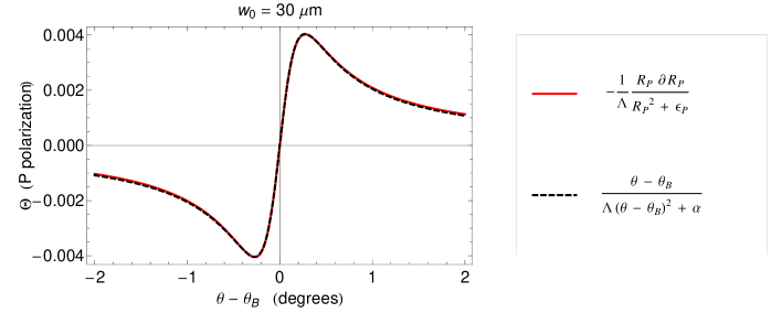
Figure 2: Geometry of beam reflection at the air-medium interface.

III Alternative route

Both Goos-Hänchen and Imbert-Fedorov shifts can be calculated in an alternative manner that displays the both spatial and angular characters of the shifts. The starting point is Eq. (34) we rewrite here as

$$\mathbf{E}^{R}(\mathbf{r}) =\iint\limits_{-\infty}^{\hphantom{xxii}\infty}\bm{E}(U,V)e^{iWZ}e^{i\left(-UX_{r}+VY_{r}\right)}\;\mathrm{d}U\,\mathrm{d}V,$$ (53)

where $Z=Z_{r}+D$ and

$$\bm{E}(U,V) =\sum_{\lambda=1}^{2}\hat{\mathbf{e}}_{\lambda}(\widetilde{\mathbf{k}})r_{\lambda}(U,V)E_{\lambda}(U,V).$$ (54)

After a straightforward calculation, it is not difficult to prove the validity of the following formulas:

$$\iint\limits_{-\infty}^{\hphantom{xxii}\infty}\lvert\mathbf{E}^{R}(X,Y,Z)\rvert^{2}\;\mathrm{d}X\,\mathrm{d}Y =\iint\limits_{-\infty}^{\hphantom{xxii}\infty}\lvert\bm{E}(U,V)\rvert^{2}\;\mathrm{d}U\,\mathrm{d}V,$$ (55)

$$\iint\limits_{-\infty}^{\hphantom{xxii}\infty}X\lvert\mathbf{E}^{R}(X,Y,Z)\rvert^{2}\;\mathrm{d}X\,\mathrm{d}Y =-i\iint\limits_{-\infty}^{\hphantom{xxii}\infty}\frac{\partial\bm{E}}{\partial U}\cdot\bm{E}^{*}\;\mathrm{d}U\,\mathrm{d}V-Z\iint\limits_{-\infty}^{\hphantom{xxii}\infty}\frac{U}{W}\lvert\bm{E}\rvert^{2}\;\mathrm{d}U\,\mathrm{d}V,$$ (56)

$$\iint\limits_{-\infty}^{\hphantom{xxii}\infty}Y\lvert\mathbf{E}^{R}(X,Y,Z)\rvert^{2}\;\mathrm{d}X\,\mathrm{d}Y =i\iint\limits_{-\infty}^{\hphantom{xxii}\infty}\frac{\partial\bm{E}}{\partial V}\cdot\bm{E}^{*}\;\mathrm{d}U\,\mathrm{d}V+Z\iint\limits_{-\infty}^{\hphantom{xxii}\infty}\frac{V}{W}\lvert\bm{E}\rvert^{2}\;\mathrm{d}U\,\mathrm{d}V.$$ (57)

Thus, we easily obtain

$$\left\langle X\right\rangle =\frac{\displaystyle{-i\iint\limits_{-\infty}^{\hphantom{xxii}\infty}\frac{\partial\bm{E}}{\partial U}\cdot\bm{E}^{*}\;\mathrm{d}U\,\mathrm{d}V}}{\displaystyle{\iint\limits_{-\infty}^{\hphantom{xxii}\infty}\lvert\bm{E}(U,V)\rvert^{2}\;\mathrm{d}U\,\mathrm{d}V}}-Z\frac{\displaystyle{\iint\limits_{-\infty}^{\hphantom{xxii}\infty}\frac{U}{W}\lvert\bm{E}\rvert^{2}\;\mathrm{d}U\,\mathrm{d}V}}{\displaystyle{\iint\limits_{-\infty}^{\hphantom{xxii}\infty}\lvert\bm{E}(U,V)\rvert^{2}\;\mathrm{d}U\,\mathrm{d}V}},$$ (58)

$$\left\langle Y\right\rangle =\frac{\displaystyle{i\iint\limits_{-\infty}^{\hphantom{xxii}\infty}\frac{\partial\bm{E}}{\partial V}\cdot\bm{E}^{*}\;\mathrm{d}U\,\mathrm{d}V}}{\displaystyle{\iint\limits_{-\infty}^{\hphantom{xxii}\infty}\lvert\bm{E}(U,V)\rvert^{2}\;\mathrm{d}U\,\mathrm{d}V}}+Z\frac{\displaystyle{\iint\limits_{-\infty}^{\hphantom{xxii}\infty}\frac{V}{W}\lvert\bm{E}\rvert^{2}\;\mathrm{d}U\,\mathrm{d}V}}{\displaystyle{\iint\limits_{-\infty}^{\hphantom{xxii}\infty}\lvert\bm{E}(U,V)\rvert^{2}\;\mathrm{d}U\,\mathrm{d}V}}.$$ (59)

The equations above show clearly the spatial and the angular contributions to the shifts. The angular part is the part proportional to $Z$. It is interesting to note that the $Z$-dependence is strictly linear, as these equations are exact. Moreover, if we remember that $U=k_{x_{i}}$ and $W=k_{z_{i}}$, then it is obvious that

$$\frac{U}{W}=\tan\theta_{x},\qquad\text{and}\qquad\frac{V}{W}=\tan\theta_{y}.$$ (60)

From Eq. (60) it immediately follows that

$$\frac{\partial\left\langle X\right\rangle}{\partial Z} =-\left\langle\tan\theta_{x}\right\rangle\simeq-\left\langle\theta_{x}\right\rangle,$$ (61)

$$\frac{\partial\left\langle Y\right\rangle}{\partial Z} =\left\langle\tan\theta_{y}\right\rangle\simeq\left\langle\theta_{y}\right\rangle.$$ (62)

References

• Brewster (1815) D. Brewster, Philos. Trans. R. Soc. London 105, 125 (1815).
• Mandel and Wolf (1995) L. Mandel and E. Wolf, Optical coherence and quantum optics (Cambridge University Press, Cambridge, UK, 1995), 1st ed.
• Aiello and Woerdman (2008) A. Aiello and J. P. Woerdman, Opt. Lett. 33, 1437 (2008).
• Fainman and Shamir (1984) Y. Fainman and J. Shamir, Appl. Opt. 23, 3188 (1984).
• Born and Wolf (2003) M. Born and E. Wolf, Principles of optics (Cambridge University Press, Cambridge, UK, 2003), 7th ed.
• Gragg (1988) R. F. Gragg, Am. J. Phys. 56, 1092 (1988).
• (7) A. Aiello and J. P. Woerdman, arXiv:0710.1643v2 [physics.optics] (2007).
• Goos and Hanchen (1947) F. Goos and H. Hanchen, Ann. Phys. (Leipzig) 1, 333 (1947).
• de Beauregard and Imbert (1972) O. C. de Beauregard and C. Imbert, Phys. Rev. Lett. 28, 1211 (1972).
• Porras (1997) M. A. Porras, Opt. Commun. 135, 369 (1997).
• (11) This result is in agreement with Ref. Porras (1997), where the author found the same linear dependence by calculating the moments of the Wigner distribution function of the reflected beam.
• Chan and Tamir (1985) C. C. Chan and T. Tamir, Opt. Lett. 10, 378 (1985).
• Greffet and Baylard (1992) J.-J. Greffet and C. Baylard, Opt. Commun. 93, 271 (1992).