Spin resonance in a chiral helimagnet

Abstract

It is suggested that marked features of symmetry breaking mechanism and elementary excitations in chiral helimagnet come up as visible effects in electron spin resonance (ESR) profile. Under the magnetic field applied parallel and perpendicular to the helical axis, elementary excitations are respectively described by the helimagnon associated with rotational symmetry breaking and the magnetic kink crystal phonon associated with translational symmetry breaking. We demonstrate how the ESR spectra distinguish these excitations.

In magnetism, chirality means the left- or right-handedness associated with the helical order of magnetic moments. Helimagnetic order can arise from spontaneous symmetry breaking in systems with competing exchange interactionsYoshimori59 (“symmetric”helimagnets), or it can be stabilized by the Dzyaloshinkii-Moriya (DM) antisymmetric exchange interactionDzyaloshinskii ; Moriya60 , which is realized in crystals lacking rotoinversion symmetry (“chiral”helimagnets). To clarify physical outcome of the chiral spin modulation is of great interest, especially in connection with the symmetry breaking mechanism and the spectrum of elementary excitations which are quite sensitive to the direction of the applied magnetic field.

In a chiral helimagnet, under the magnetic field parallel to the helical axis, the ground state (GS) generally changes from planar spiral to conical states [Fig. 1(a)]. The incommensurate modulation period $2\pi/Q_{0}$ is fixed through $Q_{0}=\tan^{-1}(D/J)$, where $D$ and $J$ are nearest-neighbor DM  interaction and ferromagnetic exchange interaction strengthsDzyaloshinskii64 ; Izyumov84 . The GS has infinite degeneracy associated with arbitrary choice of the origin of the phase angle $\varphi_{0}$. Consequently, the rotational symmetry around the helical axis is spontaneously broken. Then, there appears helimagnetic spin-wave (chiral helimagnon) modeElliot66 as the Nambu-Goldstone (NG) mode, which is well described in conventional spin wave picture. The chiral helimagnon has been studied in the context of cubic magnet MnSiKataoka87 ; Maleyev06 and its peculiar nature has attracted much attention in its own rightKirkpatrick .

On the other hand, under the magnetic field applied perpendicular to the helical axis, the GS possesses a periodic array of the commensurate (C) and incommensurate (IC) domains partitioned by discommensurations (DCs), i.e. the internal lattice which is called magnetic kink crystal (MKC) or sometimes referred to as chiral soliton latticeDzyaloshinskii64 ; Izyumov84 is stabilized as shown in Fig. 1(b). Actually, formation of the MKC state is reported in CuB₂O₄Rosseli . This state is also regarded as non-trivial topological GS. The topological GS in chiral magnet has attracted active attention from various viewpointsMnSiSkyrmion . As the magnetic field strength increases, the spatial period of MKC lattice, $L_{\text{kink}}$, increases and finally goes to infinity at the critical field strength. Recently, we showed that this internal lattice exhibits mutual sliding which may be experimentally detectableBKO08 ; BKO09 . In this case, the GS has infinite degeneracy associated with arbitrary choice of the center of mass position. Consequently, the translational symmetry along the helical axis is spontaneously broken. Then, the elementary excitations are described by “phonon”mode of correlated kinks. What is interesting is that we can control the size of the first Brillouin zone of the MKC lattice upon changing the magnetic field strength.

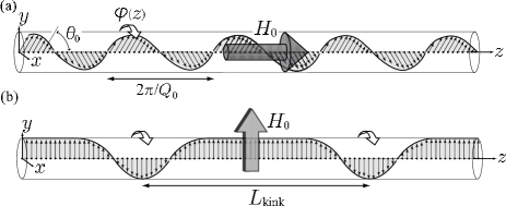
Figure 1: (a) Conical and (b) magnetic kink crystal (MKC) states. The helical axis is $z$-axis.

The elementary excitations in the kink crystal state was first investigated by SutherlandSutherland73 . He considered the sine-Gordon model for a single scalar field corresponding to the tangential $\varphi$-mode of the planar XY spins and found that the elementary excitations consist of the acoustic and optical bands separated by the energy gap. The acoustic band is formed out of correlated translations of the individual kinks and corresponds to gapless NG bosons. The optical band corresponds to renormalized Klein-Gordon bosons. In chiral helimagnet, we need to take account of not only the $\varphi$-mode but the longitudinal $\theta$-mode ($\theta$ is an angle between the spin vector and the helical axis). In previous worksBKO08 , we pointed out that the $\theta$-mode acquires an energy gap originating from the DM interaction.

Then, natural question arises as to whether the helimagnon and MKC phonon have observable consequences for the magnetic response using ESR technique. In this paper, we demonstrate how the symmetry breaking patterns and the elementary excitations come up in the ESR signals.

In the ESR experiment, the static magnetic field $\mathbf{H}_{0}$ is applied to cause Larmor precession of magnetic spins. Then supplying electromagnetic energy carried by microwave radiation, resonant absorption occurs at the precession frequency. The microwave is described as the uniform oscillating magnetic field (rf field) $\mathbf{h}(t)$ polarized in the direction perpendicular to $\mathbf{H}_{0}$ (Faraday configuration). The rf field gives rise to the Zeeman coupling with spin, $\mathcal{H}_{Z}=-\mathbf{H}(t)\cdot\mathbf{S}_{0}$, where $\mathbf{H}(t)=g_{e}\mu_{B}\mathbf{h}(t)$ ($g_{e}$ is the electron’s g-factor and $\mu_{B}$ is the Bohr magneton) and $\mathbf{S}_{0}$ is the uniform ($q=0$) component of the spin variable. For $\mathbf{H}(t)=H_{\mu}\mathbf{\hat{e}}^{\mu}\cos\left(\omega t\right)$, the ESR spectrum (absorbed energy per unit time) is given by, $\mathcal{Q}\left(\omega\right)=\omega H_{\mu}^{2}\chi_{\mu\mu}^{\prime\prime}\left(\omega\right)/2,$ where $\mathbf{\hat{e}}^{\mu}$ with $\mu=x,y,z$ denotes the unit vector along $x$, $y$, and $z$ axis [Fig. 1], respectively, and $\omega$ is a microwave frequency. The imaginary part of the dynamical susceptibility, $\chi_{\mu\nu}^{\prime\prime}\left(\omega\right)=\left(1-e^{-\hbar\omega/k_{\rm{B}}T}\right)C_{\mu\nu}\left(\omega\right)/2$, is related to the correlation function $C_{\mu\nu}\left(\omega\right)=\left\langle S_{0}^{\mu}\left(\omega\right)S_{0}^{\nu}\right\rangle$ through the fluctuation-dissipation theorem. In quantum mechanical language, the Lamor precession corresponds to equally spaced Zeeman splitting of the energy levels. Because of the equal spacing of the quantum energy levels, the quantum-classical correspondence exactly holds and the classical frequency is equal to quantum one as far as we consider Gaussian fluctuations.

First, we consider the case where the magnetic field is applied parallel to the helical axis ($z$-axis) and the rf field is polarized along the $y$-axis. Then, the elementary excitations are described as spin waves over the conical magnetic structure. A quantized spin wave is helimagnon. Then, the ESR spectrum is given by $\mathcal{Q}_{\text{hmag}}\left(\omega\right)=\omega H_{y}^{2}\chi_{yy}^{\prime\prime}\left(\omega\right)/2.$ To compute $\chi_{yy}^{\prime\prime}\left(\omega\right)$, we assume that the magnetic atoms form a three dimensional lattice and a uniform ferromagnetic coupling exists between the adjacent chains to stabilize the long-range order. Then, the Hamiltonian is interpreted as an effective one-dimensional model based on the interchain mean field picture and is written as,

$$\mathcal{H}=-{\frac{\tilde{J}}{2}}{\displaystyle\sum\limits_{j}}[e^{iQ_{0}c}S_{j}^{+}S_{j+1}^{-}+e^{-iQ_{0}c}S_{j}^{-}S_{j+1}^{+}]$$

$$-J{\displaystyle\sum\limits_{j}}S_{j}^{z}S_{j+1}^{z}+K_{\bot}{\displaystyle\sum\limits_{j}}(S_{j}^{z})^{2}-\mathbf{H}_{0}\cdot{\displaystyle\sum\limits_{j}}\mathbf{S}_{j},$$ (1)

where $\mathbf{S}_{j}$ represents a spin located at the $j$-th site along the helical axis ($z$-axis) and $S_{j}^{\pm}=S_{j}^{x}\pm iS_{j}^{y}.$ The mono-axial DM vector is $\mathbf{D}=D\mathbf{\hat{e}}^{z}$ and $\tilde{J}=|J+iD|=\sqrt{J^{2}+D^{2}}$. The lattice constant is $c$. We include the easy-plane anisotropy with strength $K_{\bot}$. For $H_{0}=0$, the planar helical structure is stable under the condition $K_{\bot}/J>1-\sqrt{1+(D/J)^{2}}$ which is assumed to be satisfied. For $0<H_{0}<H_{0c}=2S(\tilde{J}-J+K_{\bot})$, the GS is described by $S_{j}^{\pm}=Se^{\pm i\left(Q_{0}z_{j}+\varphi_{0}\right)}\sin\theta$, where the cone angle is given by $\theta=\theta_{0}=\cos^{-1}[H_{0}/\{2S(\tilde{J}-J+K_{\bot})\}].$

To obtain the spin wave spectrum, we rotate the basis frame of the crystal coordinate $\{\mathbf{\hat{e}}^{+},\mathbf{\hat{e}}^{-},\mathbf{\hat{e}}^{z}\}$ to the basis frame of the local coordinate $\{\mathbf{\hat{e}}_{j}^{+},\mathbf{\hat{e}}_{j}^{-},\mathbf{\hat{e}}_{j}^{z}\}$ where the direction of $\mathbf{\hat{e}}_{j}^{z}$ points to the equilibrium spin direction at the $j$-th siteNagamiya-review . In the spirit of conventional spin-wave approximation, we obtain the spectrum,

$$\frac{\hbar\omega_{q}}{2\tilde{J}S}=\sqrt{\left[1-\cos(qc)\right][\bar{\lambda}-\bar{\gamma}\cos(qc)]},$$ (2)

where $q$ is a wave number, $\bar{\lambda}=1+(K_{\bot}/\tilde{J})\sin^{2}\theta_{0}$ and $\bar{\gamma}=(J/\tilde{J})\sin^{2}\theta_{0}+\cos^{2}\theta_{0}$. This result reduces to the one obtained by KataokaKataoka87 and MaleyevMaleyev06 using the continuum approximation ($q\rightarrow 0$ limit). In Fig. 2(a), we show the helimagnon dispersion for $H_{0}=0,$ $0.7H_{0c},$ and $H_{0c}$. Upon increasing the field, linear dispersions for $0\leq H_{0}<H_{0c}$ continuously crosses over to the quadratic dispersion $\hbar\omega_{q}=2\tilde{J}S\left(1-\cos q\right)$ at $H_{0}=H_{0c}$. The Goldstone mode at $q=0$ corresponds to the rigid rotation of the whole helix. For $H_{0}\geq H_{0c}$, the equilibrium state is forced-ferromagnetic state and the spin wave spectrum acquire the field-induced gap.

Figure 2: (a) Helimagnon dispersions for $H_{0}/H_{0c}=0,$ $0.7,$ and $1.$. We took $D/J=0.5$ and $K_{\bot}/J=2$. Black dots indicate the location of the resonance energies. (b) Field dependence of the resonance energy as a function of $H_{0}/H_{0c}$.

Now, it is straightforward to obtain the helimagnon resonance spectrum,

$$\mathcal{Q}_{\text{hmag}}\left(\omega\right)=\frac{\pi S}{8}\omega H_{y}^{2}\delta\left(\omega-\omega_{Q_{0}}\right)$$

$$\times[(u_{Q_{0}}^{+}+u_{Q_{0}}^{-})^{2}+\cos^{2}\theta_{0}(u_{Q_{0}}^{+}-u_{Q_{0}}^{-})^{2}],$$ (3)

where $u_{Q_{0}}^{\pm}=\sqrt{\left(P/\omega_{Q_{0}}\pm 1\right)/2}$ and $P=S|2\tilde{J}+K_{\bot}\sin^{2}\theta_{0}-J\{1+\cos^{2}\theta_{0}+(J/\tilde{J})\sin^{2}\theta_{0}\}|$. Note that the external uniform field couples to the $q=\pm Q_{0}$ component of the spin wave excitation, since the field is seen in the local frame as spatially rotating field with modulation wave-number $Q_{0}$. Consequently, we have a single branch of resonance energy, as shown in Fig. 2(b). As we shall see, this situation drastically changes in the case of the MKC phonon resonance.

ESR signal in chiral helimagnet MnSi was reported by Date et al.Date77 . At that time, however, they adopted the formula obtained by YoshimoriYoshimori59 and Cooper et al.Cooper62 for symmetric helimagnetic structure stabilized by frustration among the exchange interactionsYoshimori59 . In the case of symmetric helimagnet, the spin wave dispersion exhibits dips at $q=\pm Q_{0}$ and the corresponding energy gaps vanish for $K_{\bot}=0$Nagamiya-review . There are no such additional dips in chiral helimagnon spectrum. We see, however, it may not be easy to distinguish the spin wave spectra of chiral helimagnet from those of symmetric helimagnet simply by ESR profile, because both cases give apparently quite similar field dependence of the resonance energies as shown in Fig. 2(b).

Next, we consider the MKC phonon resonance when the magnetic field is applied perpendicular to the helical axis ($y$-axis) and the rf field is polarized along the $z$-axis. The MKC state is described in terms of the slowly varying polar angles $\theta(z)$ and $\varphi(z)$. The vector spin density is defined by $\mathbf{S}\left(z\right)=\sum_{j}\mathbf{S}_{j}\delta\left(z-z_{j}\right)=\left(\sin\theta(z)\cos\varphi(z),\sin\theta(z)\sin\varphi(z),\cos\theta(z)\right).$ Then, minimizing the continuum version of the Hamiltonian (1), we obtain the MKC state as a stationary state described by $\theta=\pi/2$ and $\cos[\varphi_{0}(z)/2]=\mathrm{sn}(2Kz/L_{\text{kink}}),$ where $L_{\text{kink}}={8K}E/\pi Q_{0}$ is the period of the MKC lattice. $K$ and $E$ denote the elliptic integrals of the first and second kind, respectively, with the elliptic modulus $\kappa$ ($0\leq\kappa\leq 1$). “ sn”is Jacobi-sn function. The IC to C transition occurs at the critical field strength $H_{0}^{\ast}/{{{J}S}}=\left({\pi Q_{0}/4}\right)^{2}$ at which $L_{\text{kink}}$ diverges. The elliptic modulus $\kappa$ is determined by the condition $\sqrt{H_{0}/H_{0}^{\ast}}=\kappa/E\left(\kappa\right).$ The IC to C transition in chiral magnet is actually reported in real materialsKIY . For example, in the case of Cr_1/3NbS₂Miyadai , $H_{0}^{\ast}$ takes values from about 1 to 1.4 kOe and in the case of CuB₂O₄Kousaka , from 0.5 to 10kOe depending on temperatures.

In this case, the rf field couples with $S^{z}(z,t)=S\cos\theta(z,t)$ and ESR spectrum is given by $\mathcal{Q}_{\text{ph}}\left(\omega\right)=\omega H_{z}^{2}\chi_{zz}^{\prime\prime}\left(\omega\right)/2.$ To compute $\chi_{zz}^{\prime\prime}\left(\omega\right)$, we need the explicit form of the propagating mode $S^{z}(z,t)\simeq-Su(z,t)$ where $u({z},t)=\theta(z,t)-\pi/2$ describes small fluctuation around the MKC state. Although full description should include the $\varphi$-mode, the rf field couples to only $\theta$-mode and it is enough to consider the $\theta$-mode only. By using the mode expansion for $u(z,t)$, we set up the vibrational Hamiltonian given as collections of harmonic oscillatorsBKO08 . The explicit form of the quantized phonon wave function is given by

$$u(z,t)=\sum_{q}\sum_{n=-\infty}^{\infty}\left[\dfrac{U_{n}}{\sqrt{2\omega_{q}}}e^{-i(q-nG_{\text{MKC}})z+i\omega_{q}t}b_{q}^{\dagger}+\text{h.c.}\right],$$ (4)

where $b_{q}^{+}\left(b_{q}\right)$ are the phonon creation (annihilation) operators. The crystal-momentum $q$ and the eigenfrequency $\omega_{q}$ are expressed in terms of a real parameter $a$ running over $-K^{\prime}<a\leq K^{\prime}$, where $K^{\prime}$ is the complete elliptic integral of the first kind with the complementary modulus $\kappa^{\prime}$. For the acoustic branch, $q=l_{0}^{-1}[Z(a,\kappa^{\prime})+\pi a/(2KK^{\prime})]$ and $\hbar\omega_{q}=\varepsilon_{0}\sqrt{\Delta^{2}+\kappa^{\prime 2}\,\mathrm{sn\,}^{2}\left(a,\kappa^{\prime}\right)/2}$. For the optical branch, $q=l_{0}^{-1}[Z(a,\kappa^{\prime})+\pi a/(2KK^{\prime})+\mathrm{{dn\,}}(a,\kappa^{\prime})\mathrm{{cs\,}}(a,\kappa^{\prime})]$ and $\hbar\omega_{q}=\varepsilon_{0}\sqrt{\Delta^{2}+\mathrm{sn\,}^{-2}\left(a,\kappa^{\prime}\right)/2}$. $Z(a,\kappa^{\prime})$ is the elliptic zeta-function. We here introduced the characteristic length and energy units $l_{0}=L_{\text{kink}}/2K={4}E/\pi Q_{0}\simeq Q_{0}^{-1}$ and $\varepsilon_{0}=JS^{2}c/l_{0}=JS^{2}\pi Q_{0}c/4E\simeq DS^{2}c$, respectively. It is essential that the energy gap $\Delta=\sqrt{8E/\pi-2}$ opens at $q=0$, because of the existence of the DM interaction. The Fourier coefficients $U_{n}$ can be computed by performing contour integral of the real space wave function given in Ref. BKO08 . To obtain the ESR spectrum, we need $U_{0}=\pi/(2K\sqrt{\kappa^{\prime}})$ and $U_{n}=-i^{-1}\vartheta_{1}^{\prime-1}\vartheta_{1}(i\pi a_{n}/2K)/\sinh[\pi a_{n}/(2K)-n\pi K^{\prime}/K]$ for $n\neq 0$ [$a_{n}$ is determined by the resonance condition (6) given below]. $\vartheta_{1}$ is the Jacobi theta function and $\vartheta_{1}^{\prime}=\vartheta_{1}^{\prime}(0)$. Since $\vartheta_{1}(i\pi a/2K)$ is purely imaginary, all $U_{n}$ are real.

The reciprocal lattice constant of the MKC lattice is given by

$$G_{\text{MKC}}=\frac{2\pi}{L_{\text{kink}}}=\frac{\pi^{2}}{4KE}Q_{0}.$$ (5)

The first Brillouin zone of the MKC lattice is $\left|q\right|\leq G_{\text{MKC}}/2$ and the energy gap between the acoustic and optical branches opens at the zone boundary. As limiting forms, we have $\hbar\omega_{q}\simeq\varepsilon_{0}\sqrt{\Delta^{2}+v^{2}q^{2}}$ ($v$ is constant) for $q\ll G_{\text{MKC}}/2$ and $\hbar\omega_{q}\simeq\varepsilon_{0}\left|ql_{0}\right|/\sqrt{2}$ for $G_{\text{MKC}}/2\ll q.$ Now, we are ready to understand the ESR by the MKC phonon. Since the rf field along the $z$-axis carries the wave number $q=0$, the resonant absorption is caused by the MKC phonon modes with a series of special wave numbers

$$q=q_{n}=nG_{\text{MKC}}.$$ (6)

The correlation function can be easily computed by using Eq.(4) and we obtain the ESR absorption spectrum,

$$\mathcal{Q}_{\text{ph}}\left(\omega\right)=\frac{\pi\omega}{4}H_{z}^{2}S^{2}{\displaystyle\sum\limits_{n=0}^{\infty}}\frac{{\left|U_{n}\right|}^{2}}{\omega_{n}}\delta\left(\omega-\omega_{n}\right),$$ (7)

where $\omega_{n}=\omega_{q_{n}}$. This expression together with $U_{n}$ and $\omega_{n}$ complete a closed formula for the MKC phonon resonance. For $n=0$, the bottom of the acoustic branch ($q=0$ and $a=0$) gives $\omega_{0}=\Delta$. For $n\geq 1$, the optical branch contributes to the resonance.

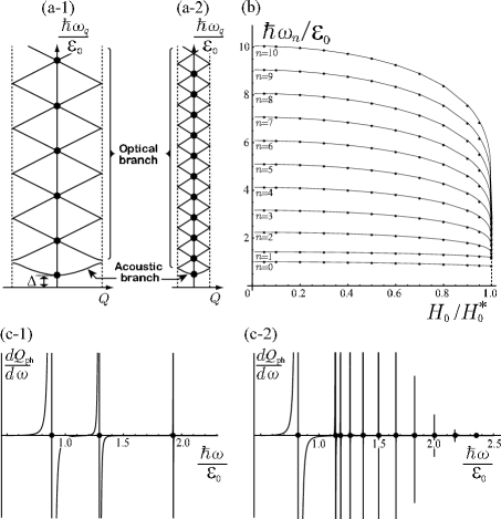
Figure 3: Energy dispersion of the MKC phonon in the reduced zone scheme for (a-1) smaller and (a-2) larger magnetic field strengths. The vertical broken lines indicate the Brillouin zone boundaries $q=\pm G_{\text{MKC}}/2.$ (b) Resonance energy $\omega_{{n}}$ for $n=0$ to $n=10$ as functions of $H_{0}/H_{0}^{\ast}$.  We took $D/J=0.5$ and $K_{\bot}/J=0$.  The derivative absorption $d\mathcal{Q}_{\text{ph}}/d\omega$ for (c-1) $H_{0}/H_{0}^{\ast}=0.8$ and (c-2) $H_{0}/H_{0}^{\ast}=1-10^{-8}$. In (a-1), (a-2), (c-1), and (c-2), black dots indicate the location of the resonance energies.

As the magnetic field increases from zero to $H_{0}^{\ast}$, $G_{\text{MKC}}$ decreases from $Q_{0}$ to zero. On the other hand, the original atomic lattice constant $c$ gives natural cutoff and the atomic Brillouin zone boundary $\pm 2\pi/c$ irrespective of the external magnetic field. Usually, $2\pi/Q_{0}\simeq 10c-100c$ and therefore $G_{\text{MKC}}$ is much smaller than the atomic zone boundary $2\pi/c.$ In Fig. 3(a), we schematically depict that the distribution of the resonance energy levels becomes more and more dense upon increasing the magnetic field strength. In Fig. 3(b), we show the resonance energies $\omega_{n}$ for $n=0$ to $n=10$ as functions of $H_{0}/H_{0}^{\ast}$. To obtain the result presented here, we first numerically solve Eq. (6) in terms of the parameter $a$, and then compute the corresponding frequency $\omega_{n}$, which completes evaluation of Eq. (7). In Fig. 3(c-1), we show the derivative absorption $d\mathcal{Q}_{\text{ph}}\left(\omega\right)/d\omega$ for $H_{0}/H_{0}^{\ast}=0.8$. The delta function is replaced by $\delta(\omega)=\pi^{-1}\epsilon/(\omega^{2}+\epsilon^{2})$ with $\epsilon=10^{-4}$. Although the weight ${\left|U_{n}\right|}^{2}$ rapidly decays for higher order resonances, the peak structure becomes visible by taking the derivative.

Of special interest is the region in the vicinity of the IC-C transition, where the distribution of the resonance levels are quite dense. In Fig. 3(c-2), we show the case for $H_{0}/H_{0}^{\ast}\rightarrow 1$. We see that a series of many densely spaced resonance lines appear. Using the relation $K(\kappa)\simeq\log(4/\sqrt{1-\kappa^{2}})$ and $E(\kappa)\simeq 1$ which hold for $\kappa\lesssim 1$, we have $\kappa\simeq\sqrt{H_{0}/H_{0}^{\ast}}$ and therefore obtain the asymptotic form of the resonance frequencies for large $n$,

$$\frac{\hbar\omega_{n}}{\varepsilon_{0}}\simeq n\frac{\pi}{K}\simeq\frac{n\pi}{\log\left(4/\sqrt{1-H_{0}/H_{0}^{\ast}}\right)}.$$ (8)

Conversely, a series of resonance fields for large $n$ are given by $H_{0n}/H_{0}^{\ast}\simeq 1-16\exp\left(-2\pi n\varepsilon_{0}/\hbar\omega\right)$ for a fixed frequency $\omega$. Our energy unit $\varepsilon_{0}\simeq DS^{2}c$ usually amounts to $J/100-J/10$, corresponding to 1meV to 10meV in energy scales. These energy scales correspond to microwave frequencies in THz region (quantitative detail depends on $\varepsilon_{0}$). So, our effects should be detectable in submillimeter wave ESR measurementsAjiro .

We stress that the MKC phonon resonance never occurs in the symmetric helimagnet due to energetic frustrationYoshimori59 , where not the MKC but the “fan” structure is stabilized under the field perpendicular to the helical axisNagamiya-review ; Cooper62 . Physical background behind this difference is that in chiral helimagnet the crystallographic chirality plays a role of “topological protectorate” for the MKC lattice state to appear as the stable GS.

In basic physical ideas, the effects we proposed here is one of examples to detect spin dynamics of phase modulated states by polarized probes such as inelastic neutron beam or X-ray. For example, neutron beams can probe the MKC phonon mode via the differential cross section $d^{2}\sigma/d\Omega d\omega\varpropto(1-\mathbf{\hat{k}}_{z}^{2})\left\langle S_{\mathbf{k}}^{z}(\omega)S_{-\mathbf{k}}^{z}\right\rangle$ where $\omega$ and $\mathbf{k}$ are respectively frequency and scattering wave-number of the neutronIzyumov-Laptev86 . Then, the scattering event occurs when both momentum conservation, $k_{z}=q-nG_{\rm{MKC}}$, and the energy conservation, $\omega=\pm\omega_{q}$, are satisfied, where $q$ is the MKC phonon wave-number. The polarized X-ray beam may also detect the MKC state via the generalized spin-orbit coupling between the spin magnetic moment and X-ray. These topics will be treated separately in a forthcoming paper.

Finally, we make theoretical comments on the MKC state. The MKC apparently seems to be one-dimensional object which is fragile against three dimensional couplings. However, it is not necessary to worry about this. Many features in physics of incommensurate magnets may be understood based on the Ginzburg-Landau free energy with a non-uniform order parameter as a function of three-dimensional coordinates. Then one should select a solution minimizing the functional that corresponds to the modulated phase. As a result of this analysis, we find a structure with a modulation along one axis in the crystal is easily stabilized. In such a case, it is enough to take into account the invariant involving derivatives with respect to one coordinate ($z$-coordinate in the present case). More rigorously speaking, we need to exclude a possibility that we have a structure with multiple modulation vectors in a single crystallographic domain. But it is known that the realization of this kind of structure is hard to occur (see for example, Ref.Izyumov_Syromyatnikov ). This is the reason why we can safely start with the effective one-dimensional model as we did in this paper.

- (1) A. Yoshimori, J. Phys. Soc. Jpn. 14, 807 (1959).
- (2) I. E. Dzyaloshinskii, J. Phys. Chem.Solids 4, 241 (1958).
- (3) T. Moriya, Phys. Rev. 120, 91 (1960).
- (4) I. E. Dzyaloshinskii, Sov. Phys. JETP 19, 960 (1964); Sov. Phys. JETP 20, 665 (1965).
- (5) Yu. A. Izyumov, Sov. Phys. Usp. 27, 845 (1984).
- (6) R. J. Elliott and R. V. Lange, Phys. Rev. 152, 235 (1966).
- (7) M. Kataoka, J. Phys. Soc. Jpn. 56, 3635 (1987).
- (8) S. V. Maleyev, Phys. Rev. B73, 174402 (2006).
- (9) D. Belitz et al., Phys. Rev. B73, 054431 (2006); Phys. Rev. B74, 024409 (2006).
- (10) B. Roessli et al., Phys. Rev. Lett. 86, 1885 (2001).
- (11) S. Mülbauer et al., Science 323, 915 (2009).
- (12) I. G. Bostrem, J. Kishine, and A. S. Ovchinnikov, Phys. Rev. B77, 132405 (2008); Phys. Rev. B78, 064425 (2008). In Fig. 4 of this paper, the Brillouin zone boundaries were incorrectly indicated and should read .
- (13) A. B. Borisov, J. Kishine, I. G. Bostrem, and A. S. Ovchinnikov, Phys. Rev. B79, 134436 (2009).
- (14) B. Sutherland, Phys. Rev. A8, 2514 (1973).
- (15) T. Nagamiya, Solid State Physics (ed. by F. Seitz, D. Turnbull and H. Ehrenreich), Vol. 20 (Academic Press, New York 1967), p.305.
- (16) M. Date, K. Okuda and K. Kadowaki, J. Phys. Soc. Jpn. 42, 1555 (1977).
- (17) B. R. Cooper et al., Phys. Rev. 127, 57 (1962).
- (18) J. Kishine, K. Inoue, and Y. Yoshida: Prog. Theoret. Phys., Supplement 159, 82 (2005).
- (19) T. Miyadai et al., J. Phys. Soc. Jpn. 52, 1394 (1983).
- (20) Y. Kousaka et al., J. Phys. Soc. Jpn.76, 123709 (2007).
- (21) Recent ESR experiments on correlated spin dynamics are reviewed in Y. Ajiro, J. Phys. Soc. Japn. 72, Suppl. B 12 (2003).
- (22) Neutron scattering by the tangential -mode was discussed in Yu. A. Izyumov and V. M. Laptev, JETP 62, 755 (1985).]
- (23) Yu. A. Izyumov, V. N. Syromyatnikov, “Phase transitions and crystal symmetry,”(Springer, 1990).