Polarizable vacuum analysis of the gravitational metric tensor

Abstract

The gravitational metric tensor implies a variable dielectric tensor of vacuum around gravitational matter. The curved spacetime in general relativity is then associated with a polarizable vacuum. It is found that the number density of the virtual dipoles in vacuum decreases with the distance from the gravitational centre. This result offers a polarizable vacuum interpretation of the gravitational force. Also, the anisotropy of vacuum polarization is briefly discussed, which appeals for observational proof of anisotropic light propagation in a vacuum altered by gravitational or electromagnetic field.

I Introduction

Ever since the establishment of general relativity, the search for the true nature of gravitational field has never ceased. In Einstein's geometric description, the gravitational force is regarded as an effect of curved spacetime. Nevertheless, Einstein himself proposed in 1920 that ``according to the general theory of relativity space is endowed with physical qualities'' Einstein1920 . Meanwhile, Eddington suggested that the deflection of light in a curved spacetime can be imaged as a refraction effect in a flat spacetime Eddington1920 . And Wilson related this refractive index to the variable specific inductive capacity of the ``ether'' near matter, i.e., suggested an electromagnetic theory of gravitation Wilson1921 . Later, in 1957, Dicke Dicke1957 , pointed out that vacuum polarization Milonni1994 ; Peskin2006 can account for such ``ether''. Recently, Puthoff reemphasized such an interpretation of gravitational field, and suggested an exponential form of the vacuum dielectric constant or vacuum refractive index Puthoff2002 . Vlokh further investigated the constitutive coefficients that could characterize the space as matter, and proposed the concept of optical-frequency dielectric impermeability perturbed by a gravitational field Vlokh2004 ; Vlokh2005 ; Vlokh2007 . The dielectric-like vacuum interpretation of gravitational field has led to successful analysis of the gravitational effects such as the gravitational red shift, the light deflection, the time delay, the gravitational lensing, and so on Dicke1957 ; Puthoff2002 ; Vlokh2004 ; Vlokh2005 ; Vlokh2007 ; Puthoff2005 ; Vlokh2006 ; Ye2008-01 ; Ye2008-02 .

In this paper, the relation between the gravitational field and the quantum vacuum will be discussed further. First, the gravitational metric tensor will be analysed and a corresponding graded refractive index in the flat spacetime will be deduced. This refractive index implies a variable dielectric tensor of the gravitational space, which is essentially related to the polarization of vacuum. Then, through the analysis of the intensity of vacuum polarization, the number density of the virtual charge pairs in vacuum will be found to be a function of the gravitational mass $M$ and the distance $r$. This analysis leads to a polarizable vacuum interpretation of the gravitational force. Finally, the anisotropic propagation of light in a vacuum will be discussed.

II From metric tensor to dielectric tensor

The general relativity states that spacetime will be curved by the gravitational matter. A curved spacetime can be described by the four-dimensional Riemann space, where the velocity of light in vacuum is defined as a constant $c$. The interval $ds=cd\tau$ ($\tau$ is the proper time) between the two adjacent points in this space is

$$ds^{2}=-g_{\mu\nu}dx^{\mu}dx^{\nu},$$ (1)

where $x^{\mu}$ is the coordinates of the point, for example, $x^{0}=ict$ ($t$ denotes the coordinate time), $x^{1}=x$, $x^{2}=y$, $x^{3}=z$, and $g_{\mu\nu}$ is the metric tensor

$$g_{\mu\nu}=\left(\begin{array}[]{cccc}g_{00}&g_{01}&g_{02}&g_{03}\\ g_{10}&g_{11}&g_{12}&g_{13}\\ g_{20}&g_{21}&g_{22}&g_{23}\\ g_{30}&g_{31}&g_{32}&g_{33}\\ \end{array}\right).$$ (2)

For a static and spherically symmetric gravitational matter with mass $M$, the Schwarzschild exterior solution gives the metric Weinberg1972

$$ds^{2}=-B(R)(icdt)^{2}-A(R)dR^{2}-R^{2}(d\theta^{2}+\sin^{2}\theta d\varphi^{2}),$$ (3)

where $B(R)=(1-2GM/Rc^{2})$, $A(R)=(1-2GM/Rc^{2})^{-1}$, and $R$, differing from the radius $r$ in flat spacetime, is the radial coordinate of the metric, $G$ is the gravitational constant, $\theta$ and $\varphi$ have the same meaning as those in the usual spherical coordinates. The above equation gives the metric tensor

$$g_{\mu\nu}=\left(\begin{array}[]{cccc}B(R)&0&0&0\\ 0&A(R)&0&0\\ 0&0&R^{2}&0\\ 0&0&0&R^{2}\sin^{2}\theta\\ \end{array}\right).$$ (4)

In a rectangular coordinate system of flat spacetime, if we set $dx^{0}=ic^{\prime}dt$ (where $c^{\prime}$, differing to the constant velocity $c$, is the velocity of light in vacuum at distance $r$ from the gravitational centre in flat spacetime), $dx=dr$, $dy=rd\theta$, $dz=r\sin\theta d\varphi$, then Eq. (3) can be rewritten as

$$ds^{2}=-B(R)\left(\frac{c}{c^{\prime}}\right)^{2}(ic^{\prime}dt)^{2}-A(R)\left(\frac{dR}{dr}\right)^{2}dx^{2}-\left(\frac{R}{r}\right)^{2}(dy^{2}+dz^{2}),$$ (5)

and the metric tensor will be

$$g^{\prime}_{\mu\nu}=\left(\begin{array}[]{cccc}B(R)\left(\frac{c}{c^{\prime}}\right)^{2}&0&0&0\\ 0&A(R)\left(\frac{dR}{dr}\right)^{2}&0&0\\ 0&0&\left(\frac{R}{r}\right)^{2}&0\\ 0&0&0&\left(\frac{R}{r}\right)^{2}\\ \end{array}\right).$$ (6)

Since the metric tensor of a flat spacetime satisfies $g^{\prime}_{00}=g^{\prime}_{11}=g^{\prime}_{22}=g^{\prime}_{33}$, we have

$$\sqrt{B(R)}\frac{c}{c^{\prime}}=\frac{R}{r},$$ (7)

$$\sqrt{A(R)}\frac{dR}{dr}=\frac{R}{r}.$$ (8)

Considering $R\rightarrow r$ at infinity, Eq. (8) gives

$$r=\frac{R}{2}\left(\sqrt{1-\frac{2GM}{Rc^{2}}}+1-\frac{GM}{Rc^{2}}\right),$$ (9)

or

$$R=r\left(1+\frac{GM}{2rc^{2}}\right)^{2}.$$ (10)

Combining Eqs. (7) and (9), we get the refractive index

$$n=\frac{c}{c^{\prime}}=\frac{1}{\frac{1}{2}\left(\sqrt{1-\frac{2GM}{Rc^{2}}}+1-\frac{GM}{Rc^{2}}\right)\sqrt{1-\frac{2GM}{Rc^{2}}}},$$ (11)

or through Eqs. (7) and (10), we get

$$n=\left(1+\frac{GM}{2rc^{2}}\right)^{3}\left(1-\frac{GM}{2rc^{2}}\right)^{-1}.$$ (12)

The above results are in agreement with those obtained through an optical way Ye2008-02 .

If we set a new tensor $\eta^{\prime}_{\mu\nu}$, each of its elements is the square root of the corresponding element of $g^{\prime}_{\mu\nu}$, then we have

$$\frac{\eta^{\prime}_{\mu\nu}}{\sqrt{1-\frac{2GM}{Rc^{2}}}}=\left(\begin{array}[]{cccc}\frac{c}{c^{\prime}}&0&0&0\\ 0&n&0&0\\ 0&0&n&0\\ 0&0&0&n\\ \end{array}\right).$$ (13)

In weak field approximation, $n=\exp\ (2GM/rc^{2})$, the tensor becomes

$$\frac{\eta^{\prime}_{\mu\nu}}{\sqrt{1-\frac{2GM}{Rc^{2}}}}=\left(\begin{array}[]{cccc}\frac{c}{c^{\prime}}&0&0&0\\ 0&\exp{\left(\frac{2GM}{rc^{2}}\right)}&0&0\\ 0&0&\exp{\left(\frac{2GM}{rc^{2}}\right)}&0\\ 0&0&0&\exp{\left(\frac{2GM}{rc^{2}}\right)}\\ \end{array}\right).$$ (14)

The above result implies a variable dielectric tensor $\varepsilon^{\prime}_{0}$ of vacuum around gravitational matter:

$$\varepsilon^{\prime}_{0}=\varepsilon_{0}\left(\begin{array}[]{ccc}\exp{\left(\frac{2GM}{rc^{2}}\right)}&0&0\\ 0&\exp{\left(\frac{2GM}{rc^{2}}\right)}&0\\ 0&0&\exp{\left(\frac{2GM}{rc^{2}}\right)}\\ \end{array}\right),$$ (15)

where $\varepsilon_{0}$ is the constant permittivity of vacuum without the influence of gravitational matter.

Eqs. (14) and (15) correspond to a graded refractive index of the vacuum

$$n=\exp{\left(\frac{2GM}{rc^{2}}\right)},$$ (16)

and a variable light velocity in gravitational field

$$c^{\prime}=c\exp{\left(-\frac{2GM}{rc^{2}}\right)}.$$ (17)

III Polarizable vacuum analysis of the tensor

It is noticed that the electric displacement vector D in a dielectric medium can be written as

$$\mathbf{D}=\mathbf{P}+\varepsilon_{0}\mathbf{E}=\mathbf{P}+\mathbf{P^{\prime}},$$ (18)

where P represents the polarization of dielectric medium, $\mathbf{P^{\prime}}=\varepsilon_{0}\mathbf{E}$ is the polarization of vacuum Dicke1957 ; Puthoff2002 ; Ye2009-01 , E denotes the electric field intensity.

For the vacuum around gravitational matter, the variable dielectric tensor expressed by Eq. (15) indicates that the intensity of vacuum polarization will be

$$\mathbf{P^{\prime}}=\varepsilon_{0}^{\prime}\mathbf{E}=\varepsilon_{0}\left(\frac{2GM}{rc^{2}}\right)\mathbf{E}.$$ (19)

As we know that, the intensity of dielectric polarization is

$$\mathbf{P}=\frac{n_{\textnormal{p}}e^{2}}{k}\mathbf{E},$$ (20)

where $n_{\textnormal{p}}$ is the number density of electric dipoles in the dielectric medium, $e$ is the electronic charge, $k$ is the stiffness factor. Similarly, we suppose the intensity of vacuum polarization to be

$$\mathbf{P^{\prime}}=\frac{n_{\textnormal{p}^{\prime}}q^{\prime 2}}{k}\mathbf{E},$$ (21)

where $n_{\textnormal{p}^{\prime}}$ is the number density of the virtual charge pairs $\pm q^{\prime}$ in the vacuum at a distance $r$ from the gravitational mass $M$. Thus we have

$$\frac{n_{\textnormal{p}^{\prime}}q^{\prime 2}}{k}=\varepsilon_{0}\left(\frac{2GM}{rc^{2}}\right),$$ (22)

or

$$n_{\textnormal{p}^{\prime}}=\frac{\varepsilon_{0}}{q^{\prime 2}}k\left(\frac{2GM}{rc^{2}}\right).$$ (23)

In general relativity, a clock at a distance $r$ from the gravitational centre is slower than that at infinity. This effect of time dilatation can be understood as the frequency reduction of the virtual dipoles in gravitational field, that is

$$\omega=\sqrt{\frac{k}{m^{\prime}}}=\omega_{0}\exp{\left(-\frac{GM}{rc^{2}}\right)},$$ (24)

where $m^{\prime}$ is the equivalent mass of a virtual dipole at distance $r$, $\omega_{0}$ is the corresponding angular frequency at infinity. Considering the energy ratio of a virtual dipole at distance $r$ to that at infinity

$$\frac{E}{E_{0}}=\frac{\hbar\omega}{\hbar\omega_{0}}=\exp\left(-\frac{GM}{rc^{2}}\right)=\frac{m^{\prime}c^{\prime 2}}{m^{\prime}_{0}c^{2}},$$ (25)

we have

$$m^{\prime}=m^{\prime}_{0}\exp\left(\frac{3GM}{rc^{2}}\right),$$ (26)

where $m^{\prime}_{0}$ is the corresponding equivalent mass at infinity.

Eqs. (24) and (26) give the relation

$$k=m^{\prime}_{0}\omega_{0}^{2}\exp\left(\frac{GM}{rc^{2}}\right)=k_{0}\exp\left(\frac{GM}{rc^{2}}\right),$$ (27)

where $k_{0}$ is the stiffness factor at infinity. Therefore

$$n_{\textnormal{p}^{\prime}}=n_{\textnormal{p}^{\prime}0}\exp\left(\frac{3GM}{rc^{2}}\right),$$ (28)

where $n_{\textnormal{p}^{\prime}0}=\varepsilon_{0}k_{0}/q^{\prime 2}$ is the number density of the virtual dipoles at infinity. This result is very similar to the number density distribution of gas molecules in a gravitational field:

$$n_{\textnormal{gas}}=n_{\textnormal{gas}0}\exp\left(-\frac{E_{\textnormal{p}}}{k_{\textnormal{B}}T}\right)=n_{\textnormal{gas}0}\exp\left(\frac{3GM}{r\overline{v^{2}}}\right),$$ (29)

where we have used the relations $E_{\textnormal{p}}=-\ GMm/r$ (the potential energy of a gas molecule) and $m\overline{v^{2}}/2=3k_{\textnormal{B}}T/2$ (the average translational kinetic energy of a molecule).

Eq. (28) can be rewritten as

$$\frac{n_{\textnormal{p}^{\prime}}}{n_{\textnormal{p}^{\prime}0}}=\frac{N/V}{N/V_{0}}=\frac{l_{0}^{3}}{l^{3}}=\exp\left(\frac{3GM}{rc^{2}}\right),$$ (30)

where $N$ is the number of virtual dipoles in a volume of $V_{0}=l_{0}^{3}$ at infinity or in a volume of $V=l^{3}$ at a distance $r$ from the gravitational centre. So we have the length relation

$$l=l_{0}\exp{\left(-\frac{GM}{rc^{2}}\right)},$$ (31)

which increases our understanding of the length contraction effect in gravitational field. It is the effects of time dilatation described by Eq. (24) and length contraction described by Eq. (31) that leads to the slowing down of the light velocity $c^{\prime}$ in a gravitational field as expressed in Eq. (17), which, in general relativity, is regarded as a constant light velocity $c$ in a curved spacetime.

IV Gravitational force

Eq. (28) tells that the number density of the virtual dipoles in vacuum decreases with the distance $r$ from the gravitational centre. This result indicates that there can be a polarizable vacuum interpretation of the gravitational force.

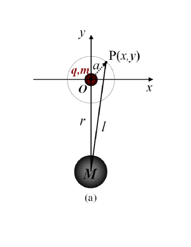
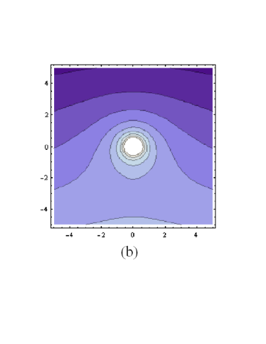
Figure 1: Consider the number density of the virtual dipoles around a $q$-charged particle in a gravitational field.

First we consider a $q$-charged particle located at a distance $r$ from a gravitational mass $M$ as shown in Fig. 1 (a). According to Eq. (28), the number density of the virtual dipoles around the charged particle is

$$n_{\textnormal{p}^{\prime}}=n_{\textnormal{p}^{\prime}0}\exp\left[\frac{3G}{c^{2}}\left(\frac{M}{l}+\frac{m}{a}\right)\right]\ \ \ \ \ \ \ \ \ \ \ \ \ \ \ \ \ \ \ \ \ \ \ \ \ \ \ \ \ \ \ \ \$$

$$=n_{\textnormal{p}^{\prime}0}\exp\left[\frac{3G}{c^{2}}\left(\frac{M}{\sqrt{x^{2}+(y+r)^{2}}}+\frac{m}{\sqrt{x^{2}+y^{2}}}\right)\right],$$ (32)

where $m$ is the mass of the particle, $a$ is the distance from the particle to a nearby point P($x$,$y$), $l$ is the distance from the point to the gravitational matter $M$. The corresponding contour map of $n_{\textnormal{p}^{\prime}}$ is shown in Fig. 1 (b), where a relatively central contour line has higher value of number density than an outer one. From the figure we know that, for a given distance $a$, the virtual dipoles in vacuum below the charged particle ($y<0$) are denser than that above the charged particle ($y>0$). Then there is a slightly higher probability for the charged particle to be coupled or ``attracted'' by the virtual dipoles at the lower side, which leads to the downward movement of the charged particle, or in other words, leads to the gravitational force on the particle.

For an electrically neutral particle or neutral matter, its inner distribution of positive and negative charges will in the same way lead to the effect of gravitational force.

V Anisotropic propagation of light in vacuum

Once the gravitational metric tensor is associated with the dielectric tensor of the vacuum, it is natural to have the idea that the tensor may be in a more general form under certain conditions, that is

$$\varepsilon^{\prime}_{0}=\varepsilon_{0}\left(\begin{array}[]{ccc}a&0&0\\ 0&b&0\\ 0&0&c\\ \end{array}\right).$$ (33)

If so, the vacuum in a specific gravitational field will exhibit its anisotropic characteristics in polarization. For example, a vacuum in a nonstatic gravitational field may no longer keep the relation of $a$=$b$=$c$ and may behave somewhat like a birefringent crystal. In such a case, there may be an anisotropic propagation of light in the gravitational field.

The gravitational birefringence in a vacuum is an analogy of the photoelastic effect. In the latter case, an isotropic material turns to be anisotropic and shows its birefringent characteristic in light propagation when a stress is applied to the material.

Similarly, if altered by a specific electric or magnetic field, an isotropic vacuum may be turned into an anisotropic one just as an isotropic dielectric medium will be. In such a case, there may be birefringence observed in the altered vacuum as the electro-optic or magneto-optic effect observed in a dielectric medium.

It is delightful that the anisotropic propagation of light in vacuum has attracted both theoretical and experimental interests in recent years Preuss2005 ; Zavattini2006 . It is hoped that substantial observational proof will be found for the birefringence of light in a gravity-or-electromagnetism-influenced vacuum.

VI Conclusions

The curved spacetime in general relativity is described by a gravitational metric tensor. It is found that this tensor corresponds to a variable dielectric tensor of vacuum around gravitational matter if viewed in a flat spacetime. In such a view, the vacuum possesses a graded refractive index, which slows down the velocity of light propagating to a gravitational body. This medium-like property of gravitational space is attributed to the virtual charge pairs in vacuum. The increasing number density of virtual dipoles towards to the gravitational centre naturally suggests a polarizable vacuum interpretation of the gravitational force. In addition, a dielectric tensor of vacuum could be in a more general form than that with equal diagonal elements, which makes it possible that a vacuum under certain conditions turns to be anisotropic. So, great importance is attached to the observations or experiments searching for anisotropic propagation of light in a vacuum modified by specific gravitational or electromagnetic fields.

Acknowledgments

This work was supported by Hangzhou Dianzi University (grant no. KYS075608069).

References

- (1) A. Einstein, Äther und Relativitätstheorie (Springer-Verlag, Berlin, 1920).
- (2) A. S. Eddington, Space, Time and Gravitation (Cambridge University Press, Cambridge, 1920).
- (3) H. A. Wilson, Phys. Rev. 17, 54 (1921).
- (4) R. H. Dicke, Rev. Mod. Phys. 29, 363 (1957).
- (5) P. W. Milonni, The Quantum Vacuum: An Introduction to Quantum Electrodynamics (Academic Press, New York, 1994).
- (6) M. E. Peskin and D. V. Schroeder, An Introduction to Quantum Field Theory (World Publishing Corp., Beijing, 2006).
- (7) H. E. Puthoff, Found. Phys. 32, 927 (2002).
- (8) R. Vlokh, Ukr. J. Phys. Opt. 5, 27 (2004).
- (9) R. Vlokh and M. Kostyrko, Ukr. J. Phys. Opt. 6, 120; 6, 125 (2005).
- (10) R. Vlokh and O. Kvasnyuk, Ukr. J. Phys. Opt. 8, 125 (2007).
- (11) H. E. Puthoff, E. W. Davis, and C. Maccone, Gen. Rel. Grav. 37, 483 (2005).
- (12) R. Vlokh and M. Kostyrko, Ukr. J. Phys. Opt. 7, 179 (2006).
- (13) X. H. Ye and Q. Lin, J. Mod. Opt. 55, 1119 (2008).
- (14) X. H. Ye and Q. Lin, J. Opt. A: Pure Appl. Opt. 10, 075001 (2008).
- (15) S. Weinberg, Gravitation and Cosmology (John Wiley and Sons, New York, 1972).
- (16) X. H. Ye, arXiv: 0902.1305v1 (2009).
- (17) O. Preuss, S. K. Solanki, M. P. Haugan, and S. Jordan, Phys. Rev. D. 72, 042001 (2005).
- (18) E. Zavattini et al., Phys. Rev. Lett. 96, 110406 (2006).