Transverse diffusion induced phase transition in asymmetric exclusion process on a surface

Abstract

We extend one dimensional asymmetric simple exclusion process (ASEP) to a surface and show that the effect of transverse diffusion is to induce a continuous phase transition from a constant density phase to a maximal current phase as the forward transition probability $p$ is tuned. The signature of the nonequilibrium transition is in the finite size effects near it. The results are compared with similar couplings operative only at the boundary. It is argued that the nature of the phases can be interpreted in terms of the modifications of boundary layers.

I Introduction

History has shown us that the study of model systems or toy models of real physical systems is the first step towards a deeper understanding of working of real physical systemspeierls . In this spirit, asymmetric simple exclusion process (ASEP) is a prototypical model of non-equilibrium statistical mechanics that deals with systems with currents flowing through them. Such systems are, in general externally driven, for example, in living cells, motor proteins, traffic flows, driven diffusive systems, transport in condensed matter and mesoscopic systems etcstinch ; ligett .

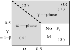
Figure 1: (a) Schematic diagram of 2-D asymmetric simple exclusion process (ASEP), with forward jump probability $p$ (thick lines) and transverse (dashed lines) excursion probability $q$, with $p+2q=1$. For $q=0$, one gets decoupled 1-D ASEP. (b)The phase diagram of 1-D and 2-D exclusion process. M $\equiv$ maximal current phase ($\rho=0.5$), in the $\alpha$-phase the bulk density is $\alpha$, and in the $\gamma$-phase it is $\gamma$. The dotted (thin solid) line is the first order (continuous) phase boundary. For the 2-D or the modified 1-D, the M region widens with $p$ inducing a transition to M in the shaded region. In the $\alpha$-phase region $p_{c}=2\alpha$ and in the $\gamma$-phase region $p_{c}=2\beta$. The points marked refer to Fig. 3

ASEP is comprised of particles moving in a particular direction with the constraint of no two particles at the same site at the same time, called simple exclusion. A particle can hop if the next site is empty. Particles are fed at one end, say $i=1$ at a rate $\alpha$ and withdrawn at $i=m(m\to\infty)$ at a rate $\beta=1-\gamma$ so that there is a current through the track. See Fig. 1(a). The main interest in ASEP has been in the steady state properties, especially the nonequilibrium phase diagrams and the stability of phases as the external parameters or drives are changed. The phase diagrams in several cases are known both for conserved and nonconserved casesevans ; derrida and an intuitive deconfinement of boundary layer approach provides a physical picture of the phase transitionssutapa ; smvm ; sutapa1 . Several variants of ASEP have also been studiedali ; jaya ; sutapa2 .

For 1-D ASEP chains, the phase diagram for the case with conservation in the bulk is shown in Fig.1(b). For large length, the phases are characterized by the density $\rho(x),x\in[0,1]$. The external drives at the boundaries maintain a density $\rho=\alpha$ at $x=0$ and $\rho=\gamma\equiv 1-\beta$ at $x=1$, and determine the fate of the bulk phase. Unlike equilibrium situations, the information of the bulk phases and phase transitions are contained in the boundary behaviour. (This can be termed a “holographic principle”). In the $\alpha$-phase of Fig.1(b), the bulk density is $\rho(x)=\alpha$ with a thin boundary layer maintaining the density at the other end. Similarly, in the $\gamma$-phase, $\rho(x)=\gamma$ in the bulk with a boundary layer at the $x=0$ end. There is a maximal current phase with $\rho(x)=0.5$ for $\alpha\geq 0.5,\gamma\leq 0.5$ with boundary layers on each side protecting the bulk. In all these cases, the boundary layers are attached to the edges. On the first order phase boundary between the $\alpha$- and the $\gamma$-phase, the density profile is $\rho(x)=\alpha+(\gamma-\alpha)x$ without any boundary layer. In case of a non-conservation in the bulk, this phase boundary gets replaced by a shock phase with localized shocks on the trackevans . This additional shock phase can be understood as a deconfinement transition of the shock from the boundarysutapa .

Here, we consider a collection of such one dimensional ASEP chains diffusively coupled to form a two dimensional ASEP (2-D ASEP). The transverse diffusion does not lead to any current in the extra dimension but affects the bulk and boundary in the preferred forward direction. An arbitrary chain may seem to have nonconservation through the leakage to or from the neighbouring chains but there is an overall bulk conservation on the lattice. We show here from simulations the existence of the maximal current phase with $\rho=0.5$ for high transverse coupling over a wider range of $\alpha$ and $\gamma$ with a phase transition to the conventional phase at a critical coupling. The phase transition behaviour in this situation can be analyzed through the changes in the boundary layers. To do so, we also consider a few variants of the model both in one and two dimensions.

II Model

Consider a modified asymmetric exclusion process (ASEP) on a sheet of $m\times n$ sites as shown in Fig. 1(a) with forward particle jump probability $p>0$ and the transverse (perpendicular to the forward direction) probability $q$ (with the constraint $p+2q=1$) provided the neighboring sites are empty. Here $q$ is a measure of the transverse coupling of the chains. For $q=0$, we get back independent 1-D ASEP chains. On the left boundary $i=1,1\leq j\leq n$ particles are injected at a rate $\alpha$ and on the right boundary $(i=m,1\leq j\leq n)$ particles are withdrawn at a rate $\beta$. The sheet is folded in a cylindrical geometry to impose periodic boundary conditions in the transverse direction i.e., sites $(i,j=1)$ are identified with sites $(i,j=n+1)$. Thus in the steady state situation we have a net particle current in the forward direction only, and no particle current in the transverse direction, because the probabilities of up- and down-hops are the same.

Figure 2: (a): Spatial density distribution $\rho(i,j)$ for a particular $j$ along the forward direction $i$ for various values of $p$ ($\alpha=\gamma=0.2$). The vertical width of any point on the line reflects the variation in the density in the transverse direction. For $p<p_{c}$ curves form one group and for $p>p_{c}$ the bulk density is determined by the left boundary $\rho(1,j)=\alpha/p$. (b): The presence of diffusing shocks for $\alpha=0.2$ and $\gamma=0.8$ when $p>p_{c}$.

II.1 Mean field analysis

The occupation number at site $(i,j)$ is $\tau_{i,j}=0$ or $1$ depending upon whether the site is empty or occupied. The rate equation governing the average particle density distribution $\rho(x,y)\equiv\langle\tau_{i,j}\rangle$ (where the average is over all realizations of the process) in the bulk is:

$$\frac{d\langle\tau_{i,j}\rangle}{dt}=p[\langle(1-\tau_{i,j})\tau_{i-1,j}\rangle-\langle(1-\tau_{i+1,j})\tau_{i,j}\rangle]+J_{ij}^{\rm{T}},\phantom{x}$$ (1a)

where the transverse part is

$$J_{ij}^{\rm{T}} = q[-\langle(1-\tau_{i,j+1})\tau_{i,j}\rangle-\langle(1-\tau_{i,j-1})\tau_{i,j}\rangle$$ (1b)

$$+\langle(1-\tau_{i,j})\tau_{i,j+1}\rangle+\langle(1-\tau_{i,j})\tau_{i,j-1}\rangle].$$

The rate equation for the two boundaries are

$$\frac{d\langle\tau_{1,j}\rangle}{dt} = +\alpha\langle 1-\tau_{1,j}\rangle-p\langle(1-\tau_{2,j})\tau_{1,j}\rangle+J_{1j}^{\rm{T}},\phantom{xxxx}$$ (1c)

$$\frac{d\langle\tau_{m,j}\rangle}{dt} = -\beta\langle\tau_{m,j}\rangle+p\langle(1-\tau_{m,j})\tau_{m-1,j}\rangle+J_{mj}^{\rm{T}}.\hfill$$ (1d)

It is interesting to note an invariance in the above equations known as the particle-hole symmetry. It implies that if we change $\alpha$ to $1-\beta$ and $\beta$ to $1-\alpha$ with $\tau$ changed to $1-\tau$, the equations of the process remains invariant.

Figure 3: The density phase transition for various values of $\alpha$ and $\beta$ in (a) 2-D and (b) 1-D cases. The average bulk density $\bar{\rho}=0.5$ up to $p<p_{c}$, but varies with $p$ for $p>p_{c}$. For both, curve (1) is for $\alpha=0.8$, $\beta=0.2$, curve (2) for $\alpha=0.2$, $\beta=0.2$, curve (3) for $\alpha=0.8$, $\beta=0.8$, and curve (4) is for $\alpha=0.2$, $\beta=0.8$, as marked in Fig. 1 (b). All these have same $p_{c}$.

In a mean-field independent-site approximation, one sees that $\rho=$constant is a solution of the bulk equation in the steady state. The phase of the system is then determined by the boundary conditions. It transpires that a constant density cannot satisfy in general both the boundary conditions. This importance of the boundary, i.e., the choice of one, both or none of the boundary conditions, is at the heart of the phase transitions. One can in addition do a stability analysis to see that a constant bulk density is indeed a stable solutionMolera . With the Boltzmann approximation (neglecting nearest neighbour correlations) i.e., $\langle\tau_{i,j}(1-\tau_{i\pm 1,j\pm 1})\rangle\equiv\langle\tau_{i,j}\rangle(1-\langle\tau_{i\pm 1,j\pm 1}\rangle),$, we take $\langle\tau_{i,j}\rangle=\rho_{0}+\delta\rho(i,j,t)$, with $\delta\rho$ a small perturbation. In terms of the Fourier modes,

$$\delta{\rho({\bf{k}},t)}=\sum_{x,y}e^{-ik_{x}x-ik_{y}y}\delta\rho(x,y,t),\qquad k_{x(y)}=\frac{2\pi q_{x(y)}}{L},$$ (2)

where $L$ is the dimension of the lattice, and $\bf{k}$ denotes $\{k_{x},k_{y}\}$, Eq. 1a can be written as

$$\frac{d\delta{\rho({\bf{k}},t)}}{dt}=\Omega(p,q,{\bf{k}})\delta{\rho({\bf{k}},t)},$$ (3)

with

$$\Omega(p,q,{\bf{k}})=ip\sin k_{x}(2\rho_{0}-1)+p\cos k_{x}+(1-p)\cos k_{y}-1.$$ (4)

Since $p\cos k_{x}+(1-p)\cos k_{y}-1<0$, the negativity of the real part of $\Omega$ insures decaying perturbations and stability. This linear stability analysis, though useful in the context of traffic jams in similar two-dimensional modelsMolera , is not enough for ASEP.

II.2 Simulation

To simulate the process for any $p$ we use a random sequential update scheme. Starting from a random distribution, we allow the system to reach a steady state. From the simulations we study the spatial density distribution and currents for various values of $p$ and for various sizes of the lattice.

To analyze in detail the density dependence on $p$, let us define the average bulk density $\bar{\rho}(p)$ (for given $\alpha$ and $\beta$),

$$\bar{\rho}(p)=\frac{1}{N}\sum_{cyc=1}^{N}\frac{1}{n^{\prime}}\sum_{i,j\subset A_{center}}\tau_{i,j}(p).$$ (5)

The averaging in Eq.(5) is done on a strip ($A_{center}$) at the center of the cylinder i.e.,$(m/2-4<i<m/2+4,1<j<n)$), and $n^{\prime}$ ($=9\times n$ in our case) is the number of sites in the central strip $A_{center}$. $N$ in the above expression is the total number of cycles of the simulation $(\sim 10^{6})$ used for averaging.

Figure 4: Finite size effects near the transition for the 2-D case (a) and for 1-D (b). Data collapse is shown in (c) and (d), with $f_{x}=(p-p_{c})L^{1/\nu}$ and $f_{y}=(\rho-\rho_{c})L^{-\mu}$.

III Results

For given $\alpha$ and $\beta$, the steady state profiles are of two types as shown in Fig. 2(a) for several values of $p$. We see that for small $p$ the bulk reaches half-filling and changes over to a boundary dependent density for larger $p$. In Fig. 3, $\bar{\rho}$ is plotted as a function of $p$ for various values of $\alpha$ and $\beta$. The behaviour shown in Fig. 2(a) is evident here. For the case $\alpha>0.5$, $\beta<0.5$, the behaviour is complementary to the case $\alpha<0.5$, $\beta>0.5$. However, there is no such transition for $\alpha>0.5$, and $\beta>0.5$. The critical $p_{c}$ also depends upon the values of $\alpha$ and $\beta$ as shown in the phase diagram Fig. 1(b). We have studied an equivalent 1-D model, because the transverse periodic boundary conditions in 2-D has some similarity with 1-D. To mimic the behaviour we modify the 1-D ASEP so that a particle jumps to the next empty site not with probability $1$ but with probability $p$, i.e., particle waits with probability $1-p$. The average bulk density in this 1-D case also shows behaviour similar to the 2-D case and is shown in Fig. 3(b). One sees the phase transition with $p$. Thus, we have the following three main observations:

1. $\rho(i,j)=0.5$ for all $p$ less than $p_{c}$, for all $\alpha$ and $\beta$.

2. In the regime $p>p_{c}$, mean-field continuum approximation is valid and phase diagram resembles the 1-D phase diagram.

3. In the shaded region marked $\alpha$-phase in Fig. 1(b) $p_{c}=2\alpha$ and in the $\gamma$-phase region $p_{c}=2\beta$.

These results can be explained by examining the boundary densities. If we do a mean-field approximation in the steady-state situation of Eq. 1c, then a homogeneous density would give $(\alpha-p\rho)(1-\rho)=0$ or $\rho=\alpha/p$ for the left boundary. The bulk current is expected to be $I(p)=p\rho(1-\rho)$ (see below) as shown in Fig. 5(a). For ASEP, the bulk satisfies the left boundary condition only in the $\alpha$-phase which requires the boundary density to be less than or equal to $0.5$. Therefore a maximal current phase is expected if $\alpha/p>0.5$, i.e., $p_{c}=2\alpha$. The left boundary layer then develops (Fig.2(a)) for $p<p_{c}$. The density variation in the boundary layer vitiates the simple argument because the density gradient dependent diffusive part of the boundary current needs to be taken into account. The net boundary density is obtained by the balance of the input and the outflow consisting of the hopping and the diffusive parts. Similar argument holds in the $\gamma$-phase region for $\beta$ and $p_{c}$. For the $\gamma$-phase, the right density is $\rho=[\gamma-(1-p)]/p$ if there is no boundary layer. The bulk density is controlled by this boundary value (rather than the withdrawal rate) so that it also takes the same value as the boundary. These observations are supported by Fig. 5(a,b).

Figure 5: (a) Current $I(p)$ vs. $p$ for 2-D case. Curve marked (1) is for $\alpha=0.8$, $\beta=0.8$, curves marked (2) and (3) are for $\alpha=0.2$, $\beta=0.8$ and $\alpha=0.8$, $\beta=0.2$ respectively, and (4) for $\alpha=0.2$, $\beta=0.2$. Currents are rescaled to match the bulk value $\rho(1-\rho)$ at $p=1.0$, to correct for finite size effects. Similar result holds for currents in 1-D case also. The solid line is $I(p)=p\rho(1-\rho)$ for the parameters of curves (2) and (3). In (b) the dependence of $p_{c}$ on $\alpha$ and $\beta$ is shown. For all the curves, $\alpha+\beta=1$. The curves are: (1) $\alpha=0.85$, (2) $\alpha=0.15$,(3) $\alpha=0.75$, (4) $\alpha=0.25$, (5) $\alpha=0.65$, (6) $\alpha=0.35$, (7) $\alpha=0.55$, (8) $\alpha=0.45$, The main observation is that $p_{c}=2\alpha$ for downward curves ($\alpha$-phase region of Fig. 1(b)) and $p_{c}=2\beta$ for the up going curves ($\gamma$-phase region of Fig. 1(b)).

It is known for ASEP, that on the first order phase boundary separating the $\alpha$- and the $\gamma$-phases, there are shocks that diffuse slowly on the track vanishing or getting created at the boundaries only. Same thing happens here also on the phase boundary which is still set by $\alpha=1-\gamma$. Because of slow diffusion of the shock, the measured density in the central patch could be either that of the $\alpha$-phase or of the $\gamma$-phase. This is shown in Figs. 3 (a) and (b)). The density remains constant for $p<p_{c}$, but after this ($p>p_{c}$) average density shows an erratic behaviour, fluctuating wildlyevans . The special point where the three phase boundaries meet is now at $\alpha=p/2,\gamma=1-(p/2)$ in the $\alpha,\gamma$ plane.

The above meanfield results seem to suggest a singularity in the density as a function of $p$, because $\bar{\rho}=0.5$ for $p<p_{c}$ but $\bar{\rho}=\alpha/p$ for $p>p_{c}$. Such a singularity is expected only in the long chain limit (infinitely long system) and not in finite systems. Fig. 4(a,b) shows a strong size dependence near $p_{c}$. For equilibrium phase transitions, singularities are rounded off by finite size when the size of the system is comparable to the characteristic length scale for the transition. The finite size behaviour, especially the size dependence, then follows a finite size scaling form. In that spirit, let us make a finite size scaling ansatz for this nonequilibrium case as

$$\rho-\rho_{c}\sim L^{-\mu}f([p-p_{c}]L^{1/\nu}),$$ (6)

with,

$$\rho-\rho_{c}\sim|p-p_{c}|^{\mu\nu}\quad{\rm for\ }L\to\infty$$ (7)

where $\rho_{c}=0.5$ is the constant density for $p<p_{c}$, $L$ is the linear dimension of the system (lattice or chain),and, $\mu$, and $\nu$ are scaling indices, then, to recover the meanfield results, we need to have $\mu=\nu^{-1}$. We have used the Bhattacharjee-Seno method for data-collapsecollap . In Fig. 4(c) the data collapse scaling is shown for 2-D for which we get $p_{c}=0.40\pm 0.008,~{}~{}\mu=0.69\pm 0.07,~{}~{}\nu^{-1}=0.72\pm 0.03$. For the 1-D case (Fig. 4(d)), we have $p_{c}=0.401\pm 0.006,~{}~{}\mu=0.46\pm 0.02,~{}~{}\nu^{-1}=0.44\pm 0.06$. These are consistent with the prediction of $\mu\nu=1$. The characteristic length scale seems to diverge as $\xi\sim\mid p-p_{c}\mid^{-\nu}$ which is set by the width of the boundary layer. Meanfield analysis is not fine enough to get this length properly.

Since the current is a measure of jumps from occupied sites to nearest vacant site in the forward direction, the probability of site occupation is $\rho$, the probability of vacancy of the next site is $1-\rho$, and jump probability in the forward direction is $p$, thus, the net current in the forward direction is $I(p)=p\rho(1-\rho)$. Consequently, $I(p)=p/4$ for $p<p_{c}$, while $I(p)=\alpha(1-\alpha/p)$ for $p>p_{c}$, joining continuously at $p=p_{c}$ with a slope discontinuity. Fig. 5(a) shows the overall agreement of the measured current and this general form of the current when the correnponding $\bar{\rho}$ obtained from the simulation is used. However, finite size rounding masks the expected singularity at $p=p_{c}$ in this current plot.

Figure 6: The importance of bulk and boundary (a) the density transition is missing when we consider only boundary sites (finite $p$) and make $p=1$ in all interior sites. (b) spatial density profiles in 2-D case for various values of $p$. For $\alpha,\gamma=0.2$. Similar behaviour is observed in equivalent 1-D case.

In order to show that the above results, though boundary driven, are not a consequence of local perturbations at the boundary, we considered a variant of the model where the transverse coupling is only at the two ends. We have put $p=1$ in the all the bulk sites i.e., for sites $2\leq i\leq n-1$ and kept finite $p$ for the first and the last site, i.e., jumps from first site to second and $n-1$th site to $n$th happen with finite $p$. We see that the system self-organizes to a state with new boundaries that control the bulk density. The actual drives (the injection and withdrawal rates) passively help in creating the relevant boundary conditions. In particular, we observe that the transition induced by $p$ for the bulk case is no longer present. The behavior of average $\rho$ with $p$ is shown in Fig. 6 (a) and the corresponding density profiles are shown in Fig. 6(b) (similar profile has benn observed in 1-D case also). The behaviour of average $\rho$ with very small $p<0.05$ shows a long living transient state, due to the very small forward motion. These observations indicate that the transition is due to a co-operative phenomenon, where bulk and boundary play their role co-operatively and inter-dependent way.

IV summary

In conclusion, the continuous transition from the injection rate dominated phase to the maximal current phase has been observed as a function of forward transition probability $p$ in a two dimensional ASEP (diffusively coupled chains). The transition shows finite size effects, reminiscent of equilibrium phase transitions, and finite size scaling predicts exponents which are consistent with the mean field theory predictions. The bottleneck created at the boundary by the transverse coupling changes the effective particle densities at the two boundaries and the ensuing phase diagram can then be mapped out from the 1-d phase diagrams with $p=1$, with the multicritical point shifting to $(\alpha=\frac{p}{2},\gamma=1-\frac{p}{2})$. However no such transition can be induced if artificial bottlenecks are created at the boundaries only. In such situations, the particles organize themselves to form a new or effective boundary density which then as per the holographic principle fixes the bulk density. This reiterates that the nonequilibrium transitions observed are cooperative but boundary driven and the boundary layers contain the information about the bulk.

References

- (1) Sir Rudolf Peierls, Model-making in physics, Contemp. Phys. 21 3 (1980).
- (2) R. B. Stinchcombe, Adv. Phys. 50 431 (2001).
- (3) T. Ligett, Interacting Particle Systems: Contact, Voter and Exclusion Processes (Springer-Verlag, Berlin, 1999)
- (4) M. R. Evans, R. Juhasz and L. Santen, Phys. Rev. E 68 026117 (2003); A. Parmeggiani, T. Franosch and E. Frey, Phys. Rev. E 70, 046101 (2004).
- (5) B. Derrida, Phys. Rep. 301 65 (1998).
- (6) S. Mukherji and S. M. Bhattacharjee, J. Phys. A 38 L285 (2005).
- (7) S. Mukherji and V. Mishra, Phys. Rev. E 74 011116 (2006).
- (8) S. Mukherji, Physica A: Stat Mech and its App, 384, 83 (2007).
- (9) M. Alimohammadi, V. Karimipour, M. Khorrami, J. Stat. Phys. 97 373 (1999).
- (10) Jaya Maji and S. M. Bhattacharjee, Euro. Phys. Lett. 81 30005 (2008).
- (11) Sutapa Mukherji, Phys. Rev. E 76, 011127 (2007).
- (12) S. M. Bhattacharjee and F. Seno, J. Phys. A 34, 6375 (2001).
- (13) Jaun M. Molera, F. C. Martinez, J. A. Cuesta, and Ricardo Brito, Phys. Rev. E. 51 175 (1995).