Dynamics of Cold Atoms Crossing a One-Way Barrier

Abstract

We implemented an optical one-way potential barrier that allows ultracold ${}^{87}\mathrm{Rb}$ atoms to transmit through when incident on one side of the barrier but reflect from the other. This asymmetric barrier is a realization of Maxwell’s demon, which can be employed to produce phase-space compression and has implications for cooling atoms and molecules not amenable to standard laser-cooling techniques. The barrier comprises two focused Gaussian laser beams that intersect the focus of a far-off-resonant single-beam optical dipole trap that holds the atoms. The main barrier beam presents a state-dependent potential to incident atoms, while the repumping barrier beam optically pumps atoms to a trapped state. We investigated the robustness of the barrier asymmetry to changes in the barrier-beam separation, the initial atomic potential energy, the intensity of the second beam, and the detuning of the first beam. We performed simulations of the atomic dynamics in the presence of the barrier, showing that the initial three-dimensional momentum distribution plays a significant role, and that light-assisted collisions are likely the dominant loss mechanism. We also carefully examined the relationship to Maxwell’s demon and explicitly accounted for the apparent decrease in entropy for our particular system.

I Introduction

The transport dynamics induced by asymmetries of systems is an important paradigm in physics, dating back to Feynman’s thought-experiment of a mechanical ratchet at finite temperature Feynman et al. (1963). The point of Feynman’s analysis was to demonstrate that in thermal equilibrium, the ratchet cannot be used to “rectify” thermal fluctuations to do useful work, because Brownian motion of the ratchet mechanism itself causes it to intermittently fail in such a way as to prevent steady-state motion against a constant force. However, in nonequilibrium situations—such as a simple temperature difference—the asymmetry of a system can induce steady-state transport, and of course do work. Recently, the study of more general “ratchets,” where thermal fluctuations or time-dependent forces couple with periodic asymmetric potentials to produce steady-state directed motion Hänggi and Bartussek (1996), has become of broad interest. Ratchet systems in the form of molecular and Brownian motors Jülicher et al. (1997); Linke et al. (2005); Serreli et al. (2007) are of particular interest in understanding how controlled motion is effected in spite of thermal fluctuations, especially at the nanoscale, where such fluctuations tend to be large. Ratchets have also recently been studied in the context of the laser-cooling of atoms in asymmetric optical-lattice potentials Mennerat-Robilliard et al. (1999).

A related problem of asymmetric transport occurs for particles in the presence of asymmetric barriers. For example, asymmetric diffusion occurs in transport across membranes. A recent experiment demonstrated that asymmetric transport can be caused by an asymmetry in the shape of the membrane pores, provided that a sufficiently wide range of particle sizes is present Shaw et al. (2007). In this case, larger particles can clog the pores (but only from one side), preventing smaller particles from diffusing through the membrane in one direction. In atom optics, it is possible to realize similar “one-way barriers” or “atom diodes,” as proposed independently by Raizen et al. Raizen et al. (2005) and Ruschhaupt and Muga Ruschhaupt and Muga (2004) in slightly different contexts (with a number of subsequent refinements in the general design Ruschhaupt and Muga (2006); Ruschhaupt et al. (2006a); Ruschhaupt and Muga (2007)). These optical one-way barriers for cold atoms are asymmetric optical potentials in the sense that atoms experience a different potential depending on the direction of incidence: atoms incident from one side reflect from the barrier, while atoms incident from the other side transmit through it. Unlike the above membrane, however, this one-way action is entirely a single-particle effect, relying on optical potentials that change depending on the internal state of the atom. Note that in a closely related proposal, a combination of coherent and incoherent processes conspires to allow transport of particles from one reservoir to another, but not in the reverse direction Kim and Choi (2005).

A common theme among all the systems mentioned above is that dissipation is required to produce asymmetric transport. Ratchets, for example, typically involve overdamped motion and thus heavy dissipation. However, an interesting question is, how little dissipation is required to produce a significant asymmetry in the transport? The most straightforward answer for the optical one-way barrier here is that one photon must be spontaneously scattered per particle, since the action of the one-way barrier depends on an irreversible change in the internal state of the atom. (Presumably, though, one can construct more complicated schemes that require even less dissipation; we will show below that our one-way barrier dissipates more entropy than is required by the second law of thermodynamics.) This question is particularly relevant in the atom-optical case, since one of the main motivations in realizing one-way barriers for atoms is in developing new laser-cooling methods for atoms Raizen et al. (2005); Dudarev et al. (2005); Ruschhaupt et al. (2006b); Price et al. (2007); Ruschhaupt and Muga (2008). The idea here is that the one-way barrier can force the accumulation of atoms into a volume much smaller than the original container. The phase-space density of the atomic vapor increases if the effect of the volume compression outweighs any heating effects of the barrier. (Cooling can then be straightforwardly effected via adiabatic expansion; the most important step in terms of controlling an atomic vapor is reducing the phase-space volume.) Phase-space compression with one-way barriers has recently been demonstrated with rubidium atoms Price et al. (2008); Thorn et al. (2008). The best increase in phase-space density achieved so far is a factor of $350$ above the initial conditions of a vapor in a magnetic trap Bannerman et al. (2009). Though standard laser-cooling techniques such as Doppler cooling are now well established Metcalf and van der Straten (1999), they generally rely on the existence of a cycling optical transition: atoms falling into “dark states” decouple from the cooling lasers. Since the irreversible action of a one-way barrier relies in principle only on the scattering of a single photon, laser-cooling techniques based on one-way barriers may help circumvent problems with dark states and enable laser cooling of molecules Narevicius and Raizen (2009) and the many atoms for which standard laser-cooling methods are ineffective.

Another, more fundamental, motivation for studying the one-way barrier comes from its connection to Maxwell’s demon Maxwell (1871); Bennett (1987); Scully and Scully (2007); Ruschhaupt et al. (2006b). In this thought-experiment, the demon manipulates a trapdoor in a wall dividing a container of gas. The demon could use the trapdoor as a one-way barrier to reduce the space occupied by the atoms without performing any work, in an apparent violation of the second law of thermodynamics. (Maxwell’s original demon used the trapdoor to separate hot and cold atoms to achieve a temperature gradient, but the reduction of entropy is the essence of the thought-experiment.) One can think about the resolution to this “paradox” in a number of ways Bennett (1987); Scully and Scully (2007), but the key issue is that the demon must perform measurements on the system, gaining the information needed to perform feedback via the trapdoor. The entropy decrease of the atoms is balanced by an increase in the entropy of the demon’s memory due to the accumulated information. This cannot continue indefinitely in a cyclic process unless the demon’s memory is reset, or “erased.” The erasure requires transferring entropy to the environment, in accordance with the second law. Our experiment effectively consists of only a single thermodynamic cycle, and so a cyclic erasure is not strictly necessary. The spontaneous scattering of photons from the barrier laser light in our experiment both acts as an effective position measurement on each atom and carries away sufficient entropy to compensate for entropy lost in the reduction in phase-space volume.

This work builds on our previous study of an all-optical realization of a one-way barrier for rubidium atoms Thorn et al. (2008). Here we perform a detailed study of the dynamics of cold atoms crossing the one-way barrier. We study how various aspects of the barrier configuration contribute to its operation, and we discuss the key elements of optimizing the robustness and performance of the barrier. We also compare our data to simulations that treat the center-of-mass motion of the atoms classically, and obtain good agreement. Finally, we examine in some detail the entropic aspects of phase-space compression with the one-way barrier.

II Procedures

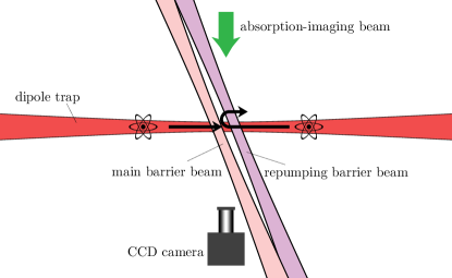
Figure 1: (Color online) Schematic diagram of the optical setup, showing the dipole trap, barrier beams, and imaging system.

Figure 2: Relevant atomic levels of ${}^{87}\mathrm{Rb}$ on the $\mathrm{D}_{2}$ cooling transition (not to scale), shown with the off-resonant coupling of the main barrier beam. Atoms with $F{=}1$ see this field as red-detuned, while $F{=}2$ atoms see a blue detuning. The repumping barrier beam is resonant with the $F{=}1\to F^{\prime}{=}2$ MOT repumping transition.

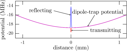
Figure 3: (Color online) Optical potentials seen by atoms along the axis of the dipole trap in our experiment. The overall trapping potential is from the main dipole-trap beam, while the narrow state-dependent feature results from the main barrier beam. The main barrier beam produces a repulsive potential for atoms in the reflecting ($F{=}2$) ground state, and an attractive potential for atoms in the transmitting ($F{=}1$) ground state.

The optical one-way barrier is the principal feature of our experimental setup (Fig. 1), comprising two focused Gaussian laser beams. The one-way barrier scheme exploits the hyperfine ground-state structure of ${}^{87}\mathrm{Rb}$ to create an asymmetry that allows atoms to transmit through the barrier when traveling in one direction, but reflects them when traveling in the other. The main barrier beam is tuned between the $F{=}1\to F^{\prime}$ and $F{=}2\to F^{\prime}$ ${}^{87}\mathrm{Rb}$ hyperfine transitions, as shown in Fig. 2. Thus the detuning $\Delta:=\omega-\omega_{0}$ of the barrier-beam frequency $\omega$ with respect to the atomic resonance $\omega_{0}$ has opposite signs for atoms in the two hyperfine ground levels. This results in the main barrier beam presenting an attractive potential to atoms in the $F{=}1$ ground state and a repulsive potential to atoms in the $F{=}2$ ground state, because the optical dipole potential is inversely proportional to the detuning $\Delta$. These two potentials are plotted in Fig. 3. To create the asymmetry, we introduce a second beam, the repumping barrier beam, that is resonant with the $F{=}1\to F^{\prime}{=}2$ repumping transition, displaced from the main barrier beam as shown in Fig. 1. If all atoms start in the transmitting ($F{=}1$) ground state, they can pass through the main barrier beam until they pass through the repumping barrier beam, at which point they will be pumped to the reflecting ($F{=}2$) ground state. The atoms will then see the main barrier beam as a potential barrier and will remain trapped on that side of the one-way barrier. We choose to have the repumping barrier beam on the right-hand side of the main barrier beam, which makes that side the reflecting side of the barrier, and the left-hand side the transmitting side.

We initially cool and trap the ${}^{87}\mathrm{Rb}$ atoms in a standard six-beam magneto-optic trap (MOT) Metcalf and van der Straten (1999), loaded from a cold atomic beam produced by a pyramid MOT Lee et al. (1996). After a secondary polarization-gradient cooling stage with reduced intensity and increased detuning of the trapping beam, we have about $2\times 10^{5}$ atoms at about $30\ \mathrm{\mu K}$ in an ultra-high vacuum of $\lesssim 10^{-10}\ \mathrm{torr}$. The position of the MOT can be shifted several millimeters in each coordinate using magnetic bias fields.

After cooling we load the atoms into a far-detuned optical dipole trap produced by a $1090(5)\ \mathrm{nm}$ Yb:fiber laser. The laser emits a collimated, multiple-longitudinal-mode, unpolarized, nearly Gaussian beam with a $1.9(1)\ \mathrm{mm}$ $1/e^{2}$ beam radius. We operate this laser so that the total power inside the vacuum chamber is $9.3(5)\ \mathrm{W}$. We focus the beam with a single $200\ \mathrm{mm}$ focal length plano-convex lens, producing a $30.9(5)\ \mathrm{\mu m}$ waist ($1/e^{2}$ intensity radius) and a $2.8\ \mathrm{mm}$ Rayleigh length. For ${}^{87}\mathrm{Rb}$ atoms in either hyperfine ground state, this beam yields a nearly conservative potential well with a maximum potential depth of $k_{{}_{\mathrm{B}}}\times 0.9\ \mathrm{mK}$. This dipole trap has longitudinal and transverse harmonic frequencies of $24\ \mathrm{Hz}$ and $3.0\ \mathrm{kHz}$, respectively (near the trap center), a $1/e$ lifetime of $20\ \mathrm{s}$, and a maximum scattering rate of only $3\ \mathrm{s^{-1}}$. Atoms are typically loaded in the anharmonic region of the trap, so that the atomic motion dephases and has a different period ($50\ \mathrm{ms}$) than the harmonic frequency suggests (angular momentum adds to this effect; see Appendix C).

The two one-way barrier beams are nearly parallel asymmetric Gaussian beams with a variable separation. Their foci nearly coincide with the focus of the dipole-trap beam, intersecting it at about $12(3)^{\circ}$ from the perpendicular to the beam axis (as in Fig. 1). The main [repumping] barrier beam has a waist of $11.5(5)\ \mathrm{\mu m}$ [$13(2)\ \mathrm{\mu m}$] along the dipole-trap axis and $80(7)\ \mathrm{\mu m}$ [$60(7)\ \mathrm{\mu m}$] perpendicular to the dipole-trap axis. We control the power of the repumping barrier beam with an acousto-optic modulator (AOM).

We measure the separation of the two beams on a beam profiler that has a resolution of $5.6\ \mathrm{\mu m/pixel}$. We take pictures of each beam profile at many locations along the beam axis near the focus, thus making it possible to accurately locate the axial position of the focus despite the fact the beam waists are on the same order of magnitude as the camera resolution. Using this setup, we determine the separation of the beams (on the order of ten microns) with an error on the order of a micron.

We image the atoms by illuminating them with a $45\ \mathrm{\mu s}$ pulse of light resonant with the $F{=}2\to F^{\prime}{=}3$ MOT trapping transition. This absorption-imaging beam is nearly perpendicular to the dipole-trap beam, and is detected by a charge-coupled-device (CCD) camera, which images the shadow left by the atoms that scatter light out of the beam. We image atoms in the $F{=}1$ ground state (which do not scatter the MOT trapping light) by turning the MOT repumping beams on slightly before and throughout the imaging pulse, ensuring that all atoms are in the $F{=}2$ ground state. The short image pulse is ideal for getting accurate spatial imaging, since the atoms cannot move much during that time. To reduce systematic errors due to interference fringes in the images, we subtract background offsets (as computed from the edge regions of the images) on a per-column basis and then integrate each column to form distributions (such as the ones shown in Fig. 4). The spatial resolution is $24.4\ \mathrm{\mu m}$ as set by the CCD pixel spacing, but the distributions are smoothed slightly for visual clarity. The total number of trapped atoms drifted slowly over time, so we often rescaled atom distributions in order to aid comparison of different data sets.

Our “canonical” data are taken as follows. We load the dipole trap with the MOT centered on the dipole-beam axis $0.95(5)\ \mathrm{mm}$ away from the dipole-trap focus for $5\ \mathrm{ms}$, trapping about $3\times 10^{4}$ atoms (measured by imaging the resonance fluorescence from the MOT light on a CCD camera) at $\sim\!100\ \mathrm{\mu K}$, with a peak one-dimensional atom density of around $4\times 10^{4}\ \mathrm{atoms/mm}$ (on the order of $10^{7}\ \mathrm{atoms/mm^{3}}$). Longer load times trap more atoms, but the atoms spread throughout the trap during loading. We used a relatively short loading time to keep the atoms localized. To allow atoms from the MOT that are not trapped in the dipole trap to fall away, we extinguish the MOT beams and wait approximately $20\ \mathrm{ms}$ (about half an oscillation period) after loading atoms into the dipole beam but before turning the barrier beams on. During this half-period delay, atoms spread in the dipole trap, reducing their apparent mean displacement from the dipole-trap focus. For example, the center of the atomic distribution for the normal $0.95(5)\ \mathrm{mm}$ mean starting offset of the atoms is only $0.58(8)\ \mathrm{mm}$ away from the dipole-trap focus after the half-period delay. Henceforth, we will quote the offset of the center of the atomic distribution after this delay.

During the half-period delay after loading atoms into the dipole trap, we optically pump the loaded atoms to the $F{=}1$ ground state by extinguishing the MOT repumping beams and then leaving the MOT trapping beams (red-detuned by $70\ \mathrm{MHz}$) on for another $7\ \mathrm{ms}$. We verified that this pumps virtually all the atoms to the $F{=}1$ ground state by using absorption imaging without the MOT repumping beams.

After the half-period delay, we turn on the barrier beams (we designate this time as $t=0$), allow the system to evolve for some time ranging from a few milliseconds to as long as a few seconds, and then image the atoms. We load atoms to either side of the barrier beams, and label data as either “transmitting side” or “reflecting side,” based on which side of the barrier beams the atoms were on at $t=0$ (when the barrier beams are turned on). Because we wait a half-period between loading the atoms and $t=0$, atoms are actually loaded on the opposite side of the barrier beams with respect to their “starting” location.

The main barrier beam was normally $34(1)\ \mathrm{\mu m}$ to the left (as seen by the camera) of the repumping barrier beam, making the left-hand (right-hand) side of the barrier beam the transmitting (reflecting) side. We normally ran the main barrier beam with $40(4)\ \mathrm{\mu W}$ of power (inside the vacuum chamber), resonant with the ${}^{85}\mathrm{Rb}$ $F{=}3\to F^{\prime}{=}3,4$ crossover dip in the rubidium saturated-absorption spectrum, which is $1.05(5)\ \mathrm{GHz}$ blue of the ${}^{87}\mathrm{Rb}$ MOT trapping transition. We normally ran the repumping barrier beam at $0.36(4)\ \mathrm{\mu W}$ (inside the vacuum chamber), and always stabilized it to the ${}^{87}\mathrm{Rb}$ $F{=}1\to F^{\prime}{=}2$ MOT repumping transition.

We use two different conventions when reporting laser detunings. When we wish to give the absolute frequency of a laser, we report the detuning as the difference between the laser frequency and the $F{=}2\to F^{\prime}{=}3$ ${}^{87}\mathrm{Rb}$ MOT transition. However, for computing optical potentials and scattering rates, we need to account for the presence of four separate excited states, and the hyperfine splitting between these states is not negligible. For these purposes, we compute and report an effective detuning. The dipole potential for each two-level transition is proportional to the squared dipole matrix element for the transition, and inversely proportional to the detuning. In order to keep a two-level-atom approximation, we average over the different excited states, using the correct dipole matrix elements and energy shifts, to obtain an effective two-level detuning. For example, in our canonical setup, our main barrier beam is tuned $1.05(5)\ \mathrm{GHz}$ to the blue of the $F{=}2\to F^{\prime}{=}3$ ${}^{87}\mathrm{Rb}$ MOT transition. When we compute an optical potential using all four excited states in the $\mathrm{D}_{2}$ manifold to obtain an effective two-level-atom detuning that gets the same answer, we find $1.12\ \mathrm{GHz}$ for atoms in the $F{=}2$ ground state, and $-5.41\ \mathrm{GHz}$ for atoms in the $F{=}1$ ground state. For computing scattering rates, we need to average squared dipole matrix elements divided by the square of the detuning. For the detunings we used, effective two-level detunings for both optical potentials and scattering rates differed by less than the accuracies quoted here.

One common variation from our canonical setup was the “$F{=}2$ setup.” For these data, during the half-period while we waited for MOT atoms to fall away, we chose to optically pump the atoms into the $F{=}2$ ground state by flashing the MOT repumping beam without the MOT trapping beam. Unless otherwise specified, we optically pumped atoms into the $F{=}1$ ground state.

Another variation we used was the “filled trap.” For these experiments we loaded the atoms to the left-hand side of the barrier beams for $110\ \mathrm{ms}$ and waited $200\ \mathrm{ms}$ before turning the barrier beams on, loading about $9\times 10^{4}$ atoms at $\sim\!100\ \mathrm{\mu K}$. These times are several times the longitudinal trap period, and so resulted in a fairly even distribution of atoms throughout the dipole trap. We used the same method described above to ensure all atoms were pumped into the $F{=}1$ ground state for these experiments.

Unless otherwise noted, the main barrier beam was linearly polarized perpendicular to the dipole-trap beam axis, and the repumping barrier beam was linearly polarized parallel to the dipole-trap beam axis. We found that beam polarization was not a critical factor in the barrier operation.

III Main Results

Figure 4: Density of atoms along the dipole trap responding to the one-way barrier. The dipole-trap focus and barrier beams are located at the horizontal origins. Each curve represents an average of $78$ [$38$ for column (e)] repetitions of the experiment. Column (a): atoms are initially in the $F{=}1$ (transmitting) state and to the left of the trap center, with no barrier present. Column (b): atoms are initially in the $F{=}1$ (transmitting) state on the left (transmitting) side of the barrier. Column (c): atoms are initially in the $F{=}2$ (reflecting) state on the left (transmitting) side of the barrier. Column (d): atoms are initially in the $F{=}1$ (transmitting) state on the right (reflecting) side of the barrier. Column (e): atoms are initially loaded relatively uniformly throughout the dipole trap (a “filled trap”) in the $F{=}1$ (transmitting) state.

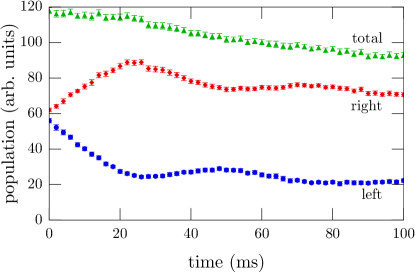
Figure 5: (Color online) Populations on the left- and right-hand sides of the one-way barrier for a “filled-trap” experiment where atoms were initially distributed throughout the dipole trap. Error bars indicate statistical error from $38$ repetitions.

The main results for the one-way barrier are presented in Fig. 4, which shows the atomic evolution in response to the one-way barrier. To elucidate the effects of the one-way barrier, Fig. 4(a) shows the evolution of the atoms in the dipole trap in the absence of the barrier. As expected, the atoms oscillate back and forth about the trap center with some breakup of the atomic cloud evident at later times due to the anharmonicity of the trapping potential and the spread in angular momentum of atoms orbiting the dipole-trap axis.

Figure 4(b) shows the dynamics of the atoms in the presence of the one-way barrier, which is located at the origin. The repumping barrier beam is positioned to the right of the main barrier beam in the columns so that the atoms, initially released from the left-hand side of the barrier, will interact first with the main barrier beam. The repumping barrier beam defines the reflecting side of the barrier, which makes the left side the transmitting side. The atoms, which are initially prepared in the $F{=}1$ transmitting state, pass through the main barrier beam to the right-hand side of the barrier. There the atoms interact with the repumping barrier beam, which optically pumps them to the $F{=}2$ reflecting state. Upon their return, the atoms are effectively trapped on the right-hand side of the barrier as they repeatedly reflect from the barrier.

When the atoms start on the reflecting side of the barrier, as in Fig. 4(d), they also remain trapped to the right of the barrier. This holds true regardless of the initial state of the atoms; atoms starting in the $F{=}2$ reflecting state are expected to reflect from the main barrier beam, while atoms starting in the $F{=}1$ transmitting state will first encounter the repumping barrier beam, which will optically pump them to the $F{=}2$ reflecting state before they reach the main barrier beam. The results presented in Fig. 4(d) show the evolution for atoms initially in the $F{=}1$ transmitting state, and we observe similarly good reflections for atoms starting in the $F{=}2$ reflecting state.

Figure 4(c) reveals what happens when atoms start on the left-hand (transmitting) side of the barrier in the $F{=}2$ (reflecting) state. Initially the atoms reflect from the barrier as expected, but then the atoms gradually pass through the barrier and become trapped on the right-hand side. This phenomenon is a direct result of choosing the main-barrier-beam frequency to be more nearly resonant with the $F{=}2\to F^{\prime}$ transition than the $F{=}1\to F^{\prime}$ transition. Though the main barrier beam reflects many atoms during the initial encounter, this interaction will also change the state of many of these atoms from the $F{=}2$ reflecting state to the $F{=}1$ transmitting state. When these atoms encounter the main barrier beam the second time, they will transmit through, while atoms that did not change state on the first reflection will eventually change their state upon subsequent reflections. This results in a net accumulation of atoms on the right-hand side of the barrier despite the atoms being initially in the “wrong” ($F{=}2$ reflecting) state. The one-way barrier functions almost equally well for atoms on either side of the barrier and for atoms in either state.

As a further test of the utility of the one-way barrier, we activated the barrier after a “filled-trap” load of the dipole trap, which resulted in a symmetric and relatively uniform initial distribution of atoms, all in the $F{=}1$ (transmitting) ground state. This experiment also had a lower barrier-beam power of $18(2)\ \mathrm{\mu W}$, chosen to reduce heating without much harm to the function of the barrier. In this scheme atoms on the left-hand side of the barrier gradually transmit to the right-hand side, while atoms on the right-hand side remain there. The results for this test are shown in Fig. 4(e), where many of the atoms that start to the left of the barrier eventually transmit to the right-hand side. Figure 5 is generated from the same data, and shows the populations on each side of the barrier as a function of time. Here it is easier to see that atoms really are being transferred from the left-hand side of the barrier to the right-hand side, in the manner of Maxwell’s demon.

III.1 Scattering

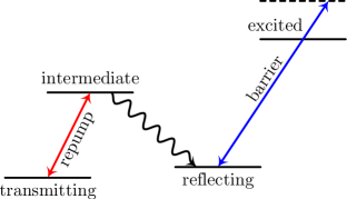
Figure 6: (Color online) Schematic of a four-level atom that would allow much larger barrier-beam detunings for reduced scattering. Here, the main barrier beam is detuned from a different transition than the one with which the repumping barrier beam is resonant. If the main-barrier-beam transition has a substantially different frequency than the repumping-barrier-beam transition, then the main barrier beam may be detuned by an amount greater than the ground-state splitting, and still create an effective barrier for atoms in the reflecting ground state while having negligible effect on atoms in the transmitting state.

The main technical challenge associated with implementing the one-way barrier lies in the limited detunings afforded by the $6.8\ \mathrm{GHz}$ ground-state hyperfine splitting of ${}^{87}\mathrm{Rb}$. Detuning the main barrier beam halfway in between the $F{=}1$ and $F{=}2$ ground states seems an obvious choice; however, this is still near enough to the $F{=}1\to F^{\prime}$ resonance to optically pump a portion of the atoms (initially in the $F{=}1$ transmitting state) to the $F{=}2$ reflecting state while they are traversing the barrier beam. This results in a sudden increase in potential energy, greatly increasing the total energy of the atom. The heating associated with this transition is on the order of the barrier height, which greatly decreases the effectiveness of the barrier. This heating mechanism informed our choice of main-barrier-beam detuning, in which the main barrier beam is more nearly resonant with the $F{=}2\to F^{\prime}$ transition, with a $1.05(5)\ \mathrm{GHz}$ detuning from the $F{=}2\to F^{\prime}{=}3$ MOT trapping transition. With this detuning, atoms in the $F{=}1$ ground state scatter few photons, so heating during transmission is minimized. Scattering during reflection is more probable because the main barrier beam is closer to the resonances available to atoms in the $F{=}2$ ground state. However, when atoms change state during reflection, their potential energy is decreased, which cools them. Those atoms are then free to transmit, and are still cool enough for the barrier to trap them when they return to the reflecting side. Data collected to probe the effects of different main-barrier-beam detunings are presented and analyzed in Sec. IV, where we see that a more symmetric detuning does not function as well as this asymmetric detuning.

For our canonical setup, which uses the detuning described above, we expect $\sim\!0.7$ scattering events on a single transmission and $\sim\!8$ scattering events on a single reflection, ignoring state changes and any scattering from the repumping barrier beam (see Appendix B). We also ran simulations (see Sec. V for more details) that account for state changes, heating, and scattering from the repumping barrier beam. These simulations found slightly higher values of $\sim\!3$ scattering events for transmission and $\sim\!10$ scattering events for a single reflection. In particular, note that even though the main barrier beam is detuned by more than half of the hyperfine ground-state splitting for transmitting atoms, scattering is not negligible.

Losses in general in this setup seem to be mainly due to light-assisted collisions (discussed in Sec. V) facilitated by the barrier beams during reflection and transmission. Light-assisted collisions include fine-structure-changing collisions Julienne and Vigué (1991), hyperfine-changing collisions Lett et al. (1995), photoassociation Miller et al. (1993), and radiative escape Gallagher and Pritchard (1989); Kuppens et al. (2000). We believe that, for our barrier beam, the dominant loss mechanism is radiative escape Gallagher and Pritchard (1989); Kuppens et al. (2000), although all can be modeled as density-dependent loss mechanisms. In radiative escape, an atom is promoted to an excited state by one of the barrier beams. While excited, the atom is much more polarizable and interacts more strongly with neighboring atoms. Before decaying, the atom accelerates toward a neighboring atom. Once the atom has decayed back to the ground state, the atoms cease interacting, but keep their kinetic energy. This kinetic energy is often enough to eject both atoms from the trap.

Initial trap lifetimes range from $300$ to $500\ \mathrm{ms}$ on the right-hand (reflecting) side of the barrier depending on the temperature of the atoms. The fitted exponential lifetimes are markedly larger (approaching $700$ to $900\ \mathrm{ms}$) in the late-time tails of the population-decay curves.

The scattering rates are not too problematic in our setup, as the lifetimes indicate. However, the lifetimes could be improved considerably if we could reduce the scattering rate by one or two orders of magnitude, so that the average number of scattering events on transmission and reflection was well below unity. As shown in Appendix B, the scattering rate depends mostly on the barrier height, atomic speed, and the ratio of the linewidth to the detuning. Once the barrier is high enough to easily trap atoms, scattering during reflection is only weakly dependent on barrier height. Scaling down the atomic velocities limits the utility of the barrier as a cooling mechanism, so increasing the detuning is perhaps the best variable to use in reducing scattering. A large increase in detuning could be achieved if the main barrier beam used a transition with a substantially different frequency than any available to the reflecting state (see Fig. 6). This would allow the main barrier beam to be far-detuned from the reflecting-to-excited state transition, and still several orders of magnitude further detuned from the transmitting-to-intermediate state transition. Atoms in the transmitting state would thus be largely unaffected by the main barrier beam because of the very large detuning, but could still be pumped to the reflecting ground state by the repumping beam. If necessary, a third laser beam detuned from the transmitting-to-intermediate state could be used to cancel any shifts of the transmitting state by the main barrier beam. This would circumvent the ground-state-splitting limitation and lead to perhaps orders of magnitude less scattering.

As a more specific example, we could use ${}^{88}\mathrm{Sr}$, with the true ground state ($5s^{2}\phantom{a}{}^{1}\mathrm{S}_{0}$) as the transmitting state and the metastable state ($5p\phantom{a}^{3}\mathrm{P}_{2}$) as the reflecting state. For the intermediate and excited states shown in Fig. 6, we could use $5p\phantom{a}^{1}\mathrm{P}_{1}$ and $5d\phantom{a}^{3}\mathrm{D}_{3}$, respectively. With these states, the main-barrier-beam transition is almost $40\ \mathrm{nm}$ red of the repumping-barrier-beam frequency and has a linewidth comparable to the ${}^{87}\mathrm{Rb}$ $\mathrm{D}_{2}$ transitions. This would allow the main barrier beam to be detuned much further than the ${}^{87}\mathrm{Rb}$ ground-state splitting and still be many nanometers detuned from the repumping-barrier-beam transition. This could reduce scattering during reflection by multiple orders of magnitude and reduce scattering during transmission to negligible levels. The repumping decays presented here are slow (millisecond time scales) and involve other states that may decay to either the reflecting state or back to the transmitting state, but all routes back to the transmitting state are short compared with the reflecting state lifetime. The long repumping time could be corrected for by allowing the repumping barrier beam to fill the entire trapping side of the barrier, allowing for more interaction time.

IV Robustness

To investigate the robustness of the one-way barrier, we varied four key parameters in the experiment:

1. the separation between the main barrier beam and the repumping barrier beam, from $8$ to $74\ \mathrm{\mu m}$;

2. the initial displacement of the atoms (this represents an effective change in barrier height), from $0$ to $0.9\ \mathrm{mm}$ on either side of the barrier;

3. the power of the repumping barrier beam, from $0.002$ to $8.7\ \mathrm{\mu W}$; and

4. the detuning of the main barrier beam from the $F{=}2$ ground state of ${}^{87}\mathrm{Rb}$, from $+0.75$ to $+4\ \mathrm{GHz}$ (blue-detuned), measured with respect to the ${}^{87}\mathrm{Rb}$ MOT trapping transition.

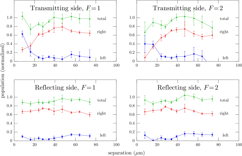
Figure 7: (Color online) Populations on the left- and right-hand sides of the one-way barrier after $100\ \mathrm{ms}$ as functions of barrier-beam separation. From left to right, top to bottom, atoms were initially loaded on the left in the $F{=}1$ ground state, on the left in the $F{=}2$ ground state, on the right in the $F{=}1$ ground state, and on the right in the $F{=}2$ ground state. Error bars indicate statistical error from at least $20$ repetitions.

Initially the separation between the beams was set to $34\ \mathrm{\mu m}$, which ensured that the tails of the Gaussian beam profiles along the dipole-trap axis overlapped slightly. We believed the overlap was necessary to prevent the atoms trapped on the right-hand side of the barrier in the $F{=}2$ reflecting state from being pumped back to the $F{=}1$ transmitting state by the main barrier beam (with an effective two-level $\Delta\approx 2\pi\times 1.12\ \mathrm{GHz}$), such that they would pass back through the barrier to the transmitting side. The presence of a small amount of repumping-barrier-beam light in the same region would rapidly pump any atoms that made it to the $F{=}1$ transmitting state back to the reflecting $F{=}2$ state. The overlap was designed to guarantee that atoms did not slowly leak back across the barrier.

Surprisingly, our studies of the effect of barrier-beam separation indicate that while overlapping the beams is important for optimizing barrier performance, it is not critical to barrier operation. Figure 7 shows populations on either side of the barrier after $100\ \mathrm{ms}$ of evolution as functions of beam separation. The transmitting-side data show the most dramatic effect for separations below about $30\ \mathrm{\mu m}$. When the beams are too close together, the tail of the repumping barrier beam can pump atoms on either side of the barrier to the reflecting state, causing the barrier to reflect atoms from both sides. This can be seen for the small separations (on the order of two beam waists and below) on the transmitting-side data, where the majority of atoms stayed on the left-hand (supposedly transmitting) side of the barrier. We also see a higher loss rate for small separations, which we suspect may be due to atoms changing state in the middle of the main barrier beam as opposed to the tail, as well as changing state more frequently. When many state changes occur in the middle of the barrier beam, the large changes in potential energy result in a large amount of heating, which causes much more loss. Large separations show much less effect on the transmitting-side data, although the $F{=}2$ data seem to get worse and then improve as the separation increases past $50\ \mathrm{\mu m}$. For atoms beginning to the right of the barrier, the beam separation does not severely affect the barrier’s reflectivity, though the functionality of the barrier declines as the separation is increased beyond about $50\ \mathrm{\mu m}$. As long as the repumping barrier beam is still present to the right of the main barrier beam, most atoms will pass back through the repumping barrier beam after reflection, correcting any state changes that may have occurred. As the separation between the beams increases, more atoms may fail to make it back to the repumping barrier beam after multiple reflections, explaining the slow reduction in reflectivity beyond $50\ \mathrm{\mu m}$. This observation has implications for one-way barrier cooling applications that require a significant number of reflections from the barrier.

We investigated how the loading position of the atoms in the dipole trap affected the dynamics of the one-way barrier as a substitute for changing the barrier height. The initial position affects the ratio of average atomic kinetic energy to barrier height, and so makes a decent substitute for varying the barrier height. However, it is important to note that changing the kinetic energy without adjusting the barrier height is not quite the same as changing the barrier height without altering the kinetic energy; the two changes have different effects on the expected number of scattering events while the atoms traverse the barrier. Appendix B contains a more detailed analysis of this assertion.

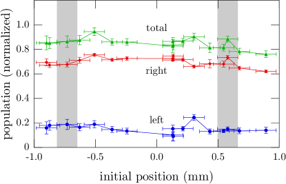
Figure 8: (Color online) Populations on the left- and right-hand sides of the one-way barrier after $100\ \mathrm{ms}$ as functions of initial loading position. The initial loading position is the position of the zero of the MOT magnetic fields relative to the focus of the dipole trap, in millimeters. Our canonical starting locations were about $0.65(8)\ \mathrm{mm}$ away from the focus of the dipole trap and are marked by the two vertical gray regions. Vertical error bars indicate statistical error from $38$ repetitions, and horizontal error bars indicate uncertainty in measuring the MOT center.

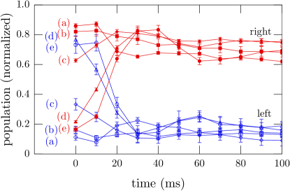
Figure 9: (Color online) Some sample time-series that formed the data in Fig. 8, showing populations on the right- and left-hand sides of the barrier as functions of time. Shown are curves for initial loading positions of (a) $0.89(8)\ \mathrm{mm}$, (b) $0.43(8)\ \mathrm{mm}$, (c) $0.14(8)\ \mathrm{mm}$, (d) $-0.51(8)\ \mathrm{mm}$, and (e) $-0.90(8)\ \mathrm{mm}$ from the barrier center. Error bars indicate statistical error from $38$ repetitions.

In Fig. 8, we plot the atomic populations in the one-way barrier at $100\ \mathrm{ms}$ as functions of initial loading position, as determined by the location of the center of the MOT trapping fields. We see no obvious effect of the loading position on the efficiency of the one-way barrier. Figure 9 shows some sample time-series for various initial loading positions. Essentially, we see that atoms starting on the transmitting side are transferred to the reflecting side, and atoms starting on the reflecting side are kept there, independently of initial loading position. This indicates that the efficiency of our one-way barrier is fairly insensitive to the velocity of the incident atoms.

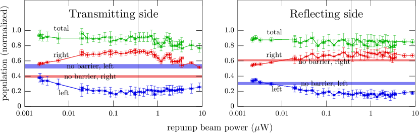
Figure 10: (Color online) Populations on the left- and right-hand sides of the one-way barrier after $100\ \mathrm{ms}$ as functions of repumping-barrier-beam power. The left panel shows results where the atoms were initially on the left-hand (transmitting) side of the barrier, and the right panel shows results where the atoms were initially on the right-hand (reflecting) side. The vertical lines in the plots show our usual repumping-barrier-beam power of $0.36\ \mathrm{\mu W}$. The two horizontal bars show the ending populations from data taken with no barriers [the one shown in column (a) of Fig. 4 and a similar data set where atoms were initially on the other side of the barrier]. The no-barrier cases show unequal left- and right-hand populations due to the oscillations of the atoms. Error bars indicate statistical error from at least $38$ repetitions.

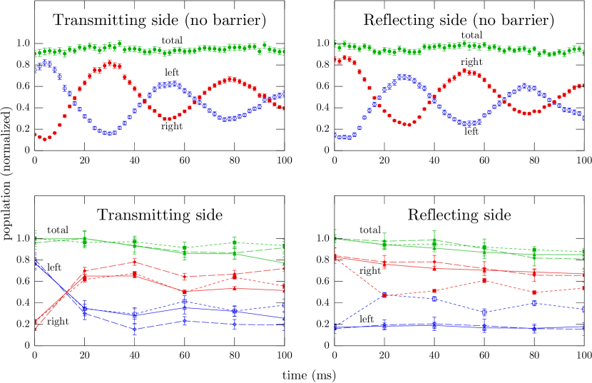
Figure 11: (Color online) Populations on the left- and right-hand sides of the one-way barrier for a few different repumping-barrier-beam powers as functions of time. The top two panels show data collected without barrier beams. The bottom two panels are generated from the same data used in Fig. 10. The data with the dotted line and squares correspond to the minimum beam power (about $2\ \mathrm{nW}$) shown in Fig. 10. The data with the dashed line and diamonds correspond to approximately the same power used to collect our canonical data. The data with the solid line and triangles correspond to the maximum beam power (about $9\ \mathrm{\mu W}$) shown in Fig. 10. The top curve in each panel shows the total population, while the other solid symbols show the right-hand side population and the open symbols show the left-hand side population.

While the intensity of the main barrier beam controls the height of the barrier, the intensity of the repumping barrier beam also plays a crucial role in the transmission and reflection of atoms from the barrier. We varied the intensity of the repumping barrier beam by over three orders of magnitude to observe its effect on the functioning of the barrier. The results for atoms that started on the left-hand and right-hand sides of the barrier are presented in Fig. 10, where the populations of atoms on either side of the barrier after $100\ \mathrm{ms}$ are measured for different repumping-barrier-beam intensities. Even over the full range of intensities we studied, the barrier continued to act asymmetrically in both experiment and simulations. This can be seen in Fig. 11, which has time-series plots of the highest and lowest repumping-beam intensities we studied. The barrier continues to operate asymmetrically, although the efficiency is strongly affected.

The transmitting-side data in Fig. 10 show the expected weak optimum in repumping-barrier-beam intensity. When the repumping barrier beam is too weak to pump atoms efficiently to the reflecting state, the atoms continue to transmit through the barrier, resulting in very little asymmetry, save for whatever side the atoms happen to be on after $100\ \mathrm{ms}$. However, even at the weakest intensity used in Fig. 10, the repumping barrier beam still pumped atoms to the reflecting state and the barrier acted asymmetrically, although less efficiently. As the intensity of the repumping barrier beam is increased, the tails of its beam profile, which extend to the left (transmitting side) of the main barrier beam, will eventually have enough intensity to optically pump atoms on the left-hand side of the barrier into the reflecting state before they reach the main barrier beam. In this limit the barrier becomes reflective on both sides, such that all atoms will remain to the left of the barrier. Though we do not reach this limit in our experiment, these two limits together indicate the existence of an optimum repumping-barrier-beam intensity that we do observe in Fig. 10.

For the reflecting-side data in Fig. 10, we see the same decrease in effectiveness as the repumping barrier beam becomes too weak to pump atoms to the reflecting state. However, we do not see the same decrease in barrier efficiency as the repumping-barrier-beam intensity is increased, since a stronger repumping barrier beam just causes the barrier to reflect better. These behaviors in the high- and low-intensity limits are evident in the reflecting-side data shown in Fig. 10, where the barrier ceases to effectively block atoms as the intensity decreases but its performance improves and then saturates (presumably at the point where all atoms reflect) as the intensity increases. At $t=0$, the atoms in the dipole trap have just enough spread that the tails of the distribution cross the barrier, as can be seen at $t=0$ in Fig. 11. This is a likely explanation as to why the population on the left-hand side of the barrier is not zero in Fig. 10, even for the largest repumping-barrier-beam intensities.

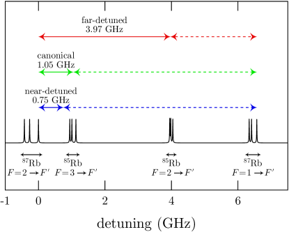
Figure 12: (Color online) A schematic of the rubidium emission spectrum around the $\mathrm{D}_{2}$ line, showing the detunings we tested for the main barrier laser. The horizontal axis measures detuning from the ${}^{87}\mathrm{Rb}$ $F{=}2\to F^{\prime}{=}3$ MOT trapping transition. Both ${}^{87}\mathrm{Rb}$ and ${}^{85}\mathrm{Rb}$ resonances are shown. Our canonical detuning coincides with the ${}^{85}\mathrm{Rb}$ $F{=}3\to F^{\prime}{=}3,4$ crossover transition, and the far-detuned value coincides with the ${}^{85}\mathrm{Rb}$ $F{=}2\to F^{\prime}{=}2$ transition. For the near-detuned value, we monitored the detuning with a Fabry-Pérot cavity. Each detuning from the ${}^{87}\mathrm{Rb}$ MOT trapping transition is shown with a solid arrow. This approximates the detuning seen by atoms in the $F{=}2$ (reflecting) state. A dotted arrow shows the detuning from the ${}^{87}\mathrm{Rb}$ MOT repumping transition, which approximates the detuning seen by atoms in the $F{=}1$ (transmitting) state.

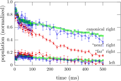
Figure 13: (Color online) Populations on the left- and right-hand sides of the one-way barrier, comparing barrier performances when the main barrier laser operates at different frequencies. For the canonical, near-detuned, and far-detuned data, the main-barrier detunings were $1.05(5)\ \mathrm{GHz}$, $0.75(5)\ \mathrm{GHz}$, and $3.97(7)\ \mathrm{GHz}$ blue of the ${}^{87}\mathrm{Rb}$ MOT transition, respectively. See Fig. 12 for details. The near-detuned and canonical data are very similar, while the far-detuned data show much more atom loss. Error bars indicate statistical error from at least $28$ repetitions.

We measured population losses for atoms released on the right-hand side of the barrier for two different main-barrier-beam detunings (shown in Fig. 12). Figure 13 shows the results. The near-detuned and far-detuned data were collected with the main barrier beam tuned $0.75(5)\ \mathrm{GHz}$ (using a Fabry-Pérot cavity) and $3.97(7)\ \mathrm{GHz}$ (using the ${}^{85}\mathrm{Rb}$ $F{=}2\to F^{\prime}{=}2$ transition) blue of the ${}^{87}\mathrm{Rb}$ MOT trapping transition, respectively. The near-detuned value was picked to be substantially closer to the $F{=}2\to F^{\prime}$ resonances than our canonical value, but not so close as to increase scattering of the barrier-beam light enough to prevent barrier operation. The far-detuned value was conveniently close to halfway between the resonances for $F{=}1$ (transmitting) and $F{=}2$ (reflecting) atoms, and is actually a little closer to the $F{=}1$ resonances. This allowed us to compare a more symmetric detuning to our canonical case and test how damaging state-changing scattering events are to the barrier operation. For both of these data sets, the intensity of the main barrier beam was adjusted so that the height of the reflecting barrier was the same as for our canonical data (with the barrier tuned to the ${}^{85}\mathrm{Rb}$ MOT transition), which is also shown in Fig. 13. The near-detuned data are nearly indistinguishable from our canonical reflecting-side data. The far-detuned data show a much shorter lifetime, but no extra leakage to the reflecting side of the barrier. This indicates the following:

1. Heating from scattering barrier-beam light alone is not much of a problem. If it were, then the near-detuned data, which should have $\sim\!2$ times as much scattering as our canonical data because it is closer to resonance, should show much more loss.

2. State-changing from scattering barrier-beam light is an issue. We believe we can explain this as follows. In both our canonical data and the near-detuned data, the barrier was much more likely to pump atoms to the transmitting state, which decreases the potential energy of the atoms, thus helping to cool them. The repumping barrier beam pumps to the reflecting state, but since that occurs away from the barrier beam, heating due to the potential-energy increase is small. In the far-detuned data, the main barrier beam can pump atoms to either state. Atoms in the transmitting state that are pumped to the reflecting state are likely to be ejected from the barrier at high speed. Atoms in the reflecting state that are pumped to the transmitting state are more likely to be moving slowly, because they were being reflected, which makes them likely to scatter again. Thus, atoms leaving the beam after a state change are more likely to have been heated than cooled. This increased heating decreases the trap lifetime substantially. Appendix B discusses scattering in more depth.

We also briefly tried having both the main barrier beam and the repumping barrier beam polarized parallel to the longitudinal axis of the dipole-trap beam. We saw no significant change, suggesting that the barrier operation is insensitive to polarization.

V Simulations

We simulated the barrier operation using a simple model where atoms were assumed to be noninteracting point particles with well-defined positions and momenta. These atoms move in conservative potentials formed by the dipole-trap beam and the main barrier beam. At every point in time the atoms were assumed to be in either the $F{=}1$ (transmitting) or $F{=}2$ (reflecting) ground state. This is because coherences between these states oscillate at much faster time scales (subnanosecond) than the center-of-mass motion (microseconds to milliseconds) of the atoms, and so can be time averaged, effectively allowing each atom to be in a classical mixture of the two ground states.

The potential the atoms move in is a sum of potentials from the dipole-trap beam and the main barrier beam. We assume the strengths of the potentials to be proportional to the local beam intensities. We use far-detuned approximations for computing the potentials, and we also use the rotating-wave and two-level-atom approximations for the barrier beams. The repumping barrier beam pumps atoms out of the $F{=}1$ ground state very quickly, and is too weak and too far detuned to produce a strong potential for atoms in the $F{=}2$ ground state, so we ignore its potential. After each time step of the integration, we compute a local scattering rate for each atom given the beam intensities at the atom’s position and the current atomic state. The dipole-trap beam is very far detuned and has a scattering rate on the order of $3\ \mathrm{s}^{-1}$, which we ignore—in our simulation only the barrier beams scatter off the atoms. We then randomly decide whether each atom scatters a photon in this time step, with a probability equal to the scattering rate times the time step. A scattering event is modeled by a randomly directed (with a dipole-emission distribution) single-photon recoil kick applied to the momentum, and a randomly chosen atomic state change based on the probabilities computed in Appendix A.

We found that the simulations were somewhat sensitive to initial conditions (compare Fig. 14 with Fig. 15). We achieved very good agreement between simulation and experiment with the following initial conditions: Atoms were initially placed in an oblong Gaussian ellipsoid, placed to match the initial conditions of the atoms in the experiment we were modeling. The long axis lies along the dipole-trap axis, with a length comparable to that measured in our experiments (we used a standard deviation of $400\ \mathrm{\mu m}$). The two short-axis widths were chosen so that most of the atoms started out trapped in the dipole trap, with some small variations to help match the simulations to the data. The momenta for each atom were initialized to random values with a $\sim\!100\ \mathrm{\mu K}$ Maxwell-Boltzmann distribution. We also simulated the nonzero loading time. For each atom we picked a uniformly distributed random start time that was less than the loading time. Each atom is frozen until its chosen start time, at which point its position and momentum begin to change according to the rules described above. This emulates the actual loading procedure, where atoms enter the dipole-trap beam and become trapped throughout the loading time. Atoms just entering the trapping region do so with random momenta because atoms in a MOT scatter often. Once trapped in the dipole trap they become dark to the MOT beams and begin evolving according to the dipole-trap potential. Thus, atoms that have spent time in the trap have a preferred direction and position different from atoms that have just been loaded, as they have begun moving toward the dipole-trap focus. This gives a slight position-momentum correlation that just-loaded atoms do not have. The intention of having a load time in the simulation was to model this correlation.

We also noticed that atoms loaded differently on one side of the barrier than on the other. This is likely due to fringes in the MOT trapping beams. Thus, in our simulations, we used two slightly different sets of initial conditions. Atoms loaded on the transmitting side of the barrier had a temperature of $100\ \mathrm{\mu K}$, with a transverse standard deviation of $16\ \mathrm{\mu m}$. Atoms loaded on the reflecting side of the barrier had a temperature of $80\ \mathrm{\mu K}$, with a transverse standard deviation of $8\ \mathrm{\mu m}$. In both cases, the atomic positions were centered about a point on the trap axis, $0.9\ \mathrm{mm}$ from the dipole-trap focus and the barrier beams.

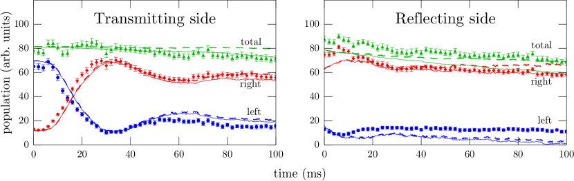
Figure 14: (Color online) Populations on the left- and right-hand sides of the one-way barrier, comparing data (points) to simulations (solid and dashed lines). The solid simulation curve has an extra light-assisted collisional loss mechanism.

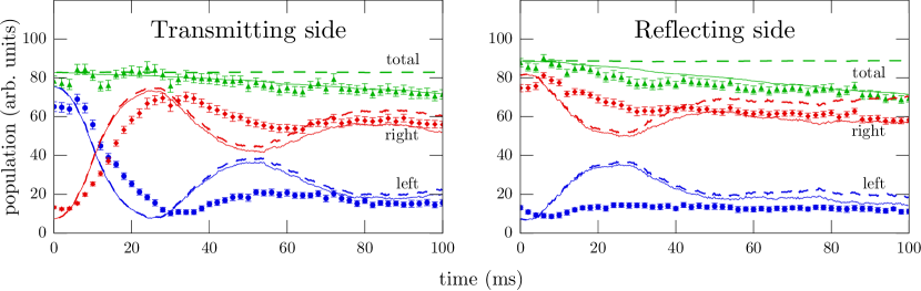
Figure 15: (Color online) Populations on the left- and right-hand sides of the one-way barrier, comparing data (points) to simulations (solid and dashed lines). These simulations and data are the same as in Fig. 14, except that the simulation initial conditions had no transverse spread in either position or momentum. These simulations do not match the data as well as the simulations in Fig. 14, illustrating how basic barrier results, such as the time atoms take to reach the barrier and whether atoms oscillate across the barrier, are strongly affected by the initial conditions. The solid simulation curve has an extra light-assisted collisional loss mechanism.

Figure 14 was derived from the same data as columns (b) and (d) of Fig. 4, but with simulation results added in for comparison. The dashed simulation curve shows the results of the simulations as described so far. As an example of how the simulations are sensitive to initial conditions, Fig. 15 shows the same experimental data as Fig. 14 compared to different simulations where the initial conditions had the same longitudinal spreads but zero transverse position and momentum spreads. These initial conditions have less kinetic energy than those used in Fig. 14, yet atoms pass through the barrier much more effectively. This is caused by an orbital effect in the dipole-trap beam, where atoms with angular momentum are slowed in their progression toward the trap focus (see Appendix C). As can be seen by comparing Fig. 14 with Fig. 15, the presence of angular momentum (Fig. 14) does effectively slow the atoms. In some of our simulations, this slowing accounts for some of the atoms remaining on the transmitting side of the barrier after $100\ \mathrm{ms}$, because they approach the barrier too slowly to even reach it on that time scale. This effect can also be seen in our experimental data (i.e., Fig. 5).

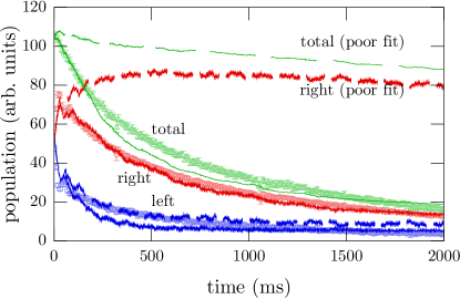
Figure 16: (Color online) Populations on the left- and right-hand sides of the one-way barrier, comparing data (points) to simulations (solid and dashed lines) for a long experiment showing the barrier lifetime. The trap was initially loaded nearly symmetrically. The dashed curve shows a simulation without including light-assisted collisions, which models the data very poorly. The solid curve shows the same simulations including light-assisted collisions, which matches the data very closely. For each curve (data and both simulations), the curves from top to bottom show the total population, the population on the right side of the barrier, and the population on the left side of the barrier. Error bars indicate statistical error from $19$ repetitions.

Figure 16 shows data taken from an experiment much like the one in Fig. 5, except with a slightly lower barrier-beam power and carried out over much longer time scales. The simulations as described (dashed line) completely miss the experiment—we needed to include light-assisted collisional losses to best fit the data. In cold-atom traps there are several mechanisms where light affects collisions between atoms Gallagher and Pritchard (1989); Julienne and Vigué (1991); Miller et al. (1993); Lett et al. (1995); Kuppens et al. (2000), which we collectively refer to as light-assisted collisions. In all of these an incident laser beam excites an atom which then decays. While the atom is excited, it either is affected by a different atom–atom potential or decays to a different state through an interaction with another atom, resulting in a large change in kinetic energy that ejects the atom (and maybe another) from the trap. Thus, all of these loss mechanisms may be collectively modeled as a density-dependent loss term with a coefficient that is proportional to the probability that atoms may be excited, although we believe that one in particular (radiative escape Kuppens et al. (2000)) is responsible for our losses.

We modeled light-assisted collisions by estimating the density of atoms in the barrier region and randomly removing them with a loss rate proportional to that density (and the beam intensity). More precisely, if we let $N$ be the number of atoms in a small volume $V$, then we expect the loss equation for $dN/dt$ to contain a term of the form $cIN^{2}/V\Delta^{2}$, where $I$ is the local laser intensity, and $\Delta$ is the detuning of the beam. Then $I/\Delta^{2}$ is approximately proportional to the scattering rate of the atoms and the $c$ coefficient is independent of volume. This is the loss term we used to model light-assisted collisions. We picked $c\sim 3\times 10^{5}\ \mathrm{cm}^{5}\,\mathrm{mW}^{-1}\,\mathrm{s}^{-3}$ to match the data shown in Fig. 16, and used that value in all other simulations.

The difference between simulations with and without light-assisted collisions can be seen in Fig. 16, where the simulation without light-assisted collisions is a very poor fit for the data, but the simulation with light-assisted collisions can be made to fit the data very well. The differences can also be seen in Fig. 14. They are not as pronounced on the shorter times scales, but the simulations with light-assisted collisions still model the data better. This suggests that light-assisted collisions are the dominant loss mechanism for our one-way barrier. Density-independent effects provide a decent (exponential) fit to the data in Fig. 16, but we know of no mechanism that could explain such a large loss rate. We can rule out any effect not directly related to the barrier beams, such as collisions with background atoms, due to the much longer lifetime of atoms in the dipole trap (about $20\ \mathrm{s}$) without the barrier beams.

If we divide our $c$ coefficient by the appropriate detuning (squared) for the experiment done by Kuppens et al. Kuppens et al. (2000), we find a coefficient of about $2\times 10^{-9}\ \mathrm{cm}^{5}\,\mathrm{mW}^{-1}\,\mathrm{s}^{-1}$. This should compare to the $K$ value of $1.1(5)\times 10^{-10}\ \mathrm{cm}^{5}\,\mathrm{mW}^{-1}\,\mathrm{s}^{-1}$ quoted in Ref. Kuppens et al. (2000). Our density-dependent loss simulations were too simplistic and approximate to expect better than order-of-magnitude agreement.

VI Connection to Maxwell’s Demon

In his 1871 Theory of Heat, Maxwell Maxwell (1871) contemplated a hypothetical creature who, being able to distinguish individual molecules in a gas, could separate hot molecules from cold molecules, resulting in a heat flow from a cold temperature to a hot temperature. This creature became known as Maxwell’s demon, and its apparent ability to violate the second law of thermodynamics remained an unsolved quandary for decades. Everyday experiences, and even the thermodynamical definition of temperature, dictate that heat flows from high to low temperatures in an irreversible fashion. This implies that separating hot and cold must decrease the entropy of a system. One can also see how such a demon could be used to perform useful work by creating a temperature differential and using an engine to extract energy from that.

Many variations of Maxwell’s demon have been proposed, including a simpler demon that allowed particles into part of a larger chamber, but not back out again—a one-way barrier Bennett (1987). Compressing the physical volume of a gas without changing the temperature also decreases entropy, and again allows for work extraction from a heat reservoir without the need for heat flow into a colder reservoir.

Today, Maxwell’s demon is usually handled through the concept of memory Bennett (1987); Scully and Scully (2007). In the case of the one-way barrier, the demon must somehow have a record of the atomic positions. If the demon knows the exact atomic positions, then to him each atom occupies a very tiny volume in phase space. By allowing the atoms into one side of the chamber, he is not really compressing phase space, but rather rearranging it. Rearranging phase space is possible via normal Hamiltonian evolution and is not a violation of the second law of thermodynamics.

If the demon does not already know the positions, the demon must somehow monitor the system and determine when to allow atoms through. A measurement must take place, and some device must take action on the result. Therefore, the measurement result must be somehow imprinted in the device. For the next measurement, either the result must be recorded elsewhere, or the first result must be erased. If the result is erased, that is an irreversible process which involves dumping entropy into the environment. If the result is not erased, then there is a memory record which goes from a known initial state to a disordered state, containing all the disorder that was removed from the atoms. Thus, entropy for the combined device system does not decrease.

As a quick example, assume we have $N$ addressable atoms distributed between two equal volumes $V_{1}$ and $V_{2}$. A demon is preparing to make sure all the atoms are in $V_{2}$, but the location of each atom within the two volumes is completely unknown. Say the demon measures the position of each atom one by one, and if they are found in $V_{1}$, then they are moved to $V_{2}$. Once it is known in which volume an atom resides, a process that swaps containers need not involve an entropy change, as the two volumes are of equal size. The demon now has a record of which volume each atom was found in. In the simplest case, this memory is a series of $N$ bits each set to $1$ or $2$. We will assume this memory to be constrained by the second law of thermodynamics. We will also assume that the initial state of the memory is known, since writing a bit over an unknown state is the same as erasing, which, as described below, requires dumping entropy into the environment.

If the demon erases the bit after each measurement, possibly to reuse it, then after each measurement the demon must reduce the phase-space volume of that bit by a factor of $2$. This is because the erasure process must take two states (representing which volume contained the particle) and map them into one (the erased state). Attempting to avoid this by measuring the state of the bit to decide how to erase it just transfers the problem to some other memory that needs to be erased. By the second law of thermodynamics, this entropy decrease of $k_{\mathrm{B}}\ln 2$ must be accompanied by a matching increase of entropy elsewhere, so that the total entropy does not decrease. After measuring and placing all $N$ atoms, the demon must have dumped $Nk_{\mathrm{B}}\ln 2$ of entropy to the outside environment.

If the demon uses $N$ different bits and does not erase them, then after the cycle is complete the memory is in one of $2^{N}$ equally likely states, since each atom was in either $V_{1}$ or $V_{2}$ with equal probability. To an outside observer the atoms are now in a smaller volume, but the state of the demon’s memory has gone from a known initial state (zero entropy) to one of $2^{N}$ possible states, which is the same entropy increase as if the demon had erased the bits and dumped that entropy into the environment. This also exactly matches the entropy decrease of the atoms being compressed from two identical volumes into one. The observer cannot know the initial atomic distribution without having made measurements of his own, either of the atomic positions or the demon’s memory. In each case there is an entropy transfer.

Here is a short computer analogy. Assume the atoms are in a one-dimensional trap, with the position represented by a number stored in memory. The volume is proportional to the number of states the number can represent, and the entropy is proportional to the logarithm of that, which is proportional to the number of digits, or bits, in that number. The first bit of the number could represent whether the atom was located in $V_{1}$ or $V_{2}$. The demon above could be thought of as taking atoms from $V_{1}$ and placing them into the exact same place within $V_{2}$. In this analogy, that means forcing the first bit of the number to $1$, effectively decreasing the size of the number by one bit. The number of total digits (entropy) did not decrease; rather, one was split off and transferred to the demon’s memory, and no longer represents part of the atom’s position.

This demon-powered barrier is similar to our one-way barrier. We can ignore extraneous effects such as photon recoil (which results in heating), unwanted scattering, and beam jitter, and still account for entropy. All that is needed is the irreversible step and the corresponding measurement record (memory) associated with it. The “memory” for our one-way barrier is the repumping barrier beam, and it accounts for the entropy even if we idealize it. The ideal repumping barrier beam changes the state of atoms from $F{=}1$ to $F{=}2$ and leaves $F{=}2$ atoms alone. That irreversible step can take place because the transitions available to the $F{=}1$ ground state are of a different frequency than those from those available to the $F{=}2$ ground state. When an atom is changed from the $F{=}1$ state to the $F{=}2$ state, a repumping-barrier-beam photon is absorbed and a different photon is emitted. Repump photons cannot change the atom from $F{=}2$ back to $F{=}1$, but the lower-frequency emitted photons can. Completely ignoring random spontaneous emission directions, we look only at whether the frequency of each photon is resonant with the $F{=}1\to F^{\prime}$ transitions or not. Each photon that is not resonant means that the number of trapped atoms was increased by one.

Let the trapping volume occupy a fraction $r$ of the total volume $V$. It can be shown that the optimum setup is to have the largest optical depth possible, and as many untrapped atoms in the trapping region as possible. The number of untrapped atoms would normally be proportional to the volume ratio $r$ of the trapping region, but could be lower if many atoms had just been trapped. In this limit each repumping-barrier-beam photon increases the number of trapped atoms with probability

$$\mathcal{P}_{\mathrm{trap}}=\frac{rN_{1}}{rN_{1}+N_{2}},$$ (1)

where $N_{1}$ is the number of untrapped atoms, $rN_{1}$ is the number of untrapped atoms in the trapping region, and $N_{2}$ is the number of trapped atoms.

Say we trap some fraction $f$ of the $N$ atoms, and it takes $P$ photons to do so. We can use the entropy of a two-part ideal gas to write out the change in entropy of the atoms (two-part because the trapped and untrapped atoms must be distinguishable if the barrier is to tell them apart). The atoms change from $N$ atoms in a volume $V$ to $\left(1-f\right)N$ untrapped atoms in a volume $V$ and $fN$ trapped atoms in a volume $rV$. The change in entropy for the atoms is

$$\Delta S_{\mathrm{a}}=k_{\scriptscriptstyle{\mathrm{B}}}N\left[f\ln r-\left(1-f\right)\ln\left(1-f\right)-f\ln f\right].$$ (2)

Likewise, the repumping photons change from $P$ identical photons to $fN$ photons in one state and $P-fN$ photons in a different state, spread throughout the same volume. However, that change is more likely to occur toward the beginning, when there are fewer trapped atoms that can become untrapped [$\mathcal{P}_{\mathrm{trap}}$ is larger when $N_{2}$ is smaller in Eq. (1)]. We can approximate the entropy increase for the repumping beam by summing up the entropy increase of the beam for each atom trapped. Each term in the sum is the expected number of photons it will take to trap the next atom times the entropy of a single photon in a mixed state, which reflects the uncertainty of whether or not the photon was emitted by a newly trapped atom. The change in entropy of the repumping beam can thus be written as

$$\Delta S_{\mathrm{r}} = -\sum_{n=0}^{fN-1}\frac{1}{\mathcal{P}_{n}}\left[\mathcal{P}_{n}\ln\mathcal{P}_{n}+\left(1-\mathcal{P}_{n}\right)\ln\left(1-\mathcal{P}_{n}\right)\right]$$

$$\mathcal{P}_{n} = \frac{rn}{rn+\left(N-n\right)},$$ (3)

where $\mathcal{P}_{n}$ is the probability of trapping another atom after $n$ atoms have been trapped, as given by Eq. (1).

Equation (2) shows a decrease in entropy from the decrease in volume, but an increase in entropy due to the multiple atom types. The increase disappears in the limit of all atoms being trapped ($f\to 1$). The repumping barrier beam shows a net increase in entropy due to the change in states of the photons. This repumping-barrier-beam entropy increase can be shown (at least in a large-number approximation) to always be at least as large as the decrease in atom entropy, so the net entropy change is non-negative. Thus, the changes in photon frequency are sufficient to uphold the second law of thermodynamics. This analysis does not include momentum diffusion for either atoms or photons resulting from photon recoil, so entropy actually increases more than is shown here.

We created a version of such a demon. Figure 5 shows data from an experiment where we had atoms spread throughout a volume, and then activated a one-way barrier in the center. The transfer was not completely efficient—not all atoms were trapped on the right-hand side of the barrier, but the spatial compression is quite good. However, the spatial compression is almost completely countered by heating from spontaneous scattering of the barrier-beam light. We found that the overall phase-space volume occupied by atoms during this experiment decreased by $7(2)\%$. Better compression is likely achievable should we optimize the setup for phase-space compression; presently we optimize the barrier for transmission rather than compression. To achieve better phase-space compression, we would use a smaller, slowly moving barrier starting initially off to one side of the atom distribution, as described by Ruschhaupt et al. Ruschhaupt et al. (2006b). At first, this barrier would capture only the atoms with the highest energies, and would do so near their turning points so that they had very little kinetic energy (allowing for a weaker barrier and less scattering). We would then adiabatically sweep the barrier along the dipole-trap axis, through the focus of the dipole trap. At each point, the barrier would trap new atoms near their turning points, where they had very little kinetic energy. The atoms that were already trapped would not gain kinetic energy. Thus when the barrier passed through the dipole-trap focus, all the atoms would be left in the center of the trap, with less kinetic energy.

VII Closing

In summary, we have demonstrated an all-optical asymmetric potential barrier capable of increasing the overall phase-space density of a sample of neutral alkali atoms. Furthermore, we have found that the barrier is robust, with fairly substantial changes having little effect, including mechanical changes, optical changes, and changes in atom-state preparation. We have also developed some theory and simulations describing the barrier.

The authors would like to thank Eryn Cook and Paul Martin for their helpful comments. This research was supported by the National Science Foundation, under Project No. PHY-0547926.

Appendix A State Changing Probabilities

Here we review the computation of approximate probabilities for linearly polarized light to change the state of an atom, for use in our simulations. In the dipole approximation, an atom must be excited by the incident light field and then spontaneously decay to a different ground state in order for the state to change. We also assume that the incident light field is a single monochromatic beam. Therefore, we wish to compute the amplitude for an atom changing from one state ($F_{0},m_{0}$) to another ($F_{1},m_{1}$), via an excited state ($F^{\prime},m^{\prime}$), and then sum over the excited states and square that sum to obtain a probability for changing states. We make the approximation that the $\mathrm{D}_{2}$ multiplet is dominant, and further that the splitting between the lines is small compared to the barrier-beam detuning. With these approximations we find the probability to be

$$P_{F_{0},m_{0}\to F_{1},m_{1}}\propto$$

$$\sum_{q^{\prime}}\left|\sum_{F^{\prime},m^{\prime}}\left\langle F_{1},m_{1}\right|\hat{d}_{q^{\prime}}\left|F^{\prime},m^{\prime}\right\rangle\left\langle F^{\prime},m^{\prime}\right|\hat{d}_{q}\left|F_{0},m_{0}\right\rangle\right|^{2},$$

where $q$ represents the polarization of the incident light, $q^{\prime}$ represents the polarization of the spontaneously emitted light ($-1$, $0$, and $+1$ for the $z$ component of angular momentum), and $\hat{d}_{q}$ and $\hat{d}_{q^{\prime}}$ are the appropriate spherical-basis dipole operators. The polarization of the incident laser field determines $q$, but we sum over all $q^{\prime}$ and all intermediate states ($F^{\prime},m^{\prime}$) within the subset of excited states that are close to the laser frequency. The $q^{\prime}$ sum is done after squaring the amplitude because different emitted polarizations are distinguishable. The ($F^{\prime},m^{\prime}$) sum is performed with the amplitudes because the near-degeneracy assumption means the different emissions are indistinguishable. Since this does not represent all possible excited states (or any ground states), the sum of $\left|F^{\prime}m^{\prime}\right\rangle\left\langle F^{\prime}m^{\prime}\right|$ is not the identity.

Next, we average over the initial magnetic sublevel $m_{0}$ and the emission polarization $q^{\prime}$ because we do not measure or simulate the magnetic sublevels of the atoms. This is also an approximation, and is partially justified by the fact that the barrier operation was not significantly affected by the incident light polarization.

Finally, we can conserve angular momentum by requiring $m^{\prime}+q^{\prime}=m_{1}$ and $m_{0}+q=m^{\prime}$. We can then evaluate Eq. (A) and perform the averages over the magnetic sublevels of ${}^{87}\mathrm{Rb}$. Given that we use linearly polarized light ($q=0$) in our experiment, we find

$$\begin{array}[]{rclcl}\displaystyle P_{\mathrm{barrier,}F{=}1\to F{=}2}&=&5/18&=&0.2\bar{7}\\ \displaystyle P_{\mathrm{barrier,}F{=}2\to F{=}1}&=&1/6&=&0.1\bar{6}.\end{array}$$ (5)

These are the values we use for the probability of a barrier-beam scattering event changing the state of an atom. The repumping barrier light is tuned close to the $F{=}1\to F^{\prime}{=}2$ transition, so we require $F^{\prime}{=}2$ in the $F^{\prime}$ sum, with the following result:

$$\begin{array}[]{rclcl}\displaystyle P_{\mathrm{repump,}F{=}1\to F{=}2}&=&1/2&=&0.5.\end{array}$$ (6)

We found that the simulations were not particularly sensitive to these probabilities, although the barrier performed better in simulations with these ratios than in simulations where all ratios were $50\%$. As a side note, we also computed the probabilities that took into account the different detunings of the excited states by weighting the excitation amplitudes in Eq. (A) by factors inversely proportional to the detunings. The probabilities then became

$$\begin{array}[]{rclcl}\displaystyle P_{\mathrm{barrier,}F{=}1\to F{=}2}&\approx&0.271\\ \displaystyle P_{\mathrm{barrier,}F{=}2\to F{=}1}&\approx&0.114\\ \displaystyle P_{\mathrm{repump,}F{=}1\to F{=}2}&\approx&0.500.\end{array}$$ (7)

These changes were not enough to significantly alter the simulations.

Appendix B Analytic scattering solution

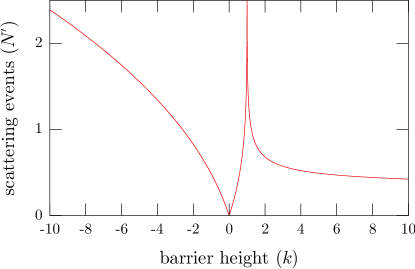
Figure 17: (Color online) Plot of Eq. (14), showing the expected number of scattering events for a two-level atom passing through a Gaussian barrier. The barrier height $k$ is defined in Eq. (11), and the number of scattering events is given as $N^{\prime}:=Nw_{0}mv_{0}\Gamma/\hbar\left|\Delta\right|$, where $N$ is the actual number of scattering events.

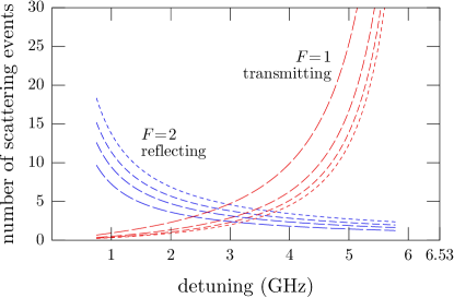
Figure 18: (Color online) Plot of Eq. (14), showing the expected number of scattering events for a quasi-two-level (ignoring state changes) ${}^{87}\mathrm{Rb}$ atom passing through a Gaussian barrier as a function of beam detuning from the $F{=}2\to F^{\prime}$ transitions. The curves that increase for larger detunings are for atoms in the $F{=}1$ transmitting state, and the curves that decrease for larger detunings are for atoms in the $F{=}2$ reflecting state. The effective detuning from the $F{=}1$ ground state for a beam tuned to the $F{=}2\to F^{\prime}$ transitions is about $6.53\ \mathrm{GHz}$. Each $F{=}1$ and $F{=}2$ pair of curves represents a different barrier height. The dotted curves show the expected numbers of scattering events for a barrier height of $k=1.25$. This means that the beam intensity for each detuning is adjusted so that the potential barrier seen by atoms in the $F{=}2$ ground state is $1.25$ times the kinetic energy of the atoms. The short-dashed curves are for $k=1.5$, the medium-dashed curves are for $k=2$, and the long-dashed curves are for $k=4$. Our canonical data had $k=2.3$ with an effective two-level detuning of $1.12\ \mathrm{GHz}$.

We can compute how many photons, on average, a two-level atom scatters while crossing a Gaussian beam if we ignore momentum kicks due to spontaneous emission. The barrier width is small compared to the Rayleigh length of the dipole trap, so we ignore any changes in the underlying potential and treat an atom in free space crossing a Gaussian potential with a scattering rate proportional to that potential. For a two-level atom in the far-detuned, rotating-wave approximation, the scattering rate is $R=\left|\Gamma V/\hbar\Delta\right|$, where $\Gamma$ is the transition linewidth, $V$ is the ac Stark shift (optical potential), and $\Delta$ is the (angular) detuning. The average number of scattering events can be computed by integrating the local scattering rate for all time, which gives

$$N=\int_{-\infty}^{\infty}R\left[x{\left(t\right)}\right]\ dt,$$ (8)

where $x(t)$ is the location of the atom at time $t$. For a Gaussian potential, we know the atom will approach the barrier and then either reflect or transmit. The expected number of scattering events up until the reflection (or passage through the barrier center) is the same as after the event, so we can restrict the integral to a period where the velocity does not change sign. This allows the change of variables to $x$, using $dt=dx/v(x)$, where $v(x)$ is the velocity of the atom when it is at position $x$. After this change of variables, we find

$$N=2\int_{x_{0}}^{\infty}\frac{R{\left(x\right)}}{v{\left(x\right)}}\ dx,$$ (9)

where $x_{0}=0$ in the case where the atom passes through the center of the barrier, and the turnaround point in the case where it does not.

If we let $w_{0}$ be the $1/e^{2}$ intensity radius of the Gaussian beam, then we can use conservation of energy to compute

$$v{\left(x\right)} v_{0}\sqrt{1-ke^{-2x^{2}/w_{0}^{2}}}$$ = (10)

$$k \frac{V_{0}}{\frac{1}{2}mv_{0}^{2}},$$ := (11)

where $v_{0}$ is the initial velocity of the atom [$v_{0}=v(x\to\infty)$], $V_{0}$ is the height of the barrier, and $k$ is defined as the ratio of the barrier height to the incident kinetic energy of the atom. We can compute $x_{0}$ by solving $v(x)=0$:

$$x_{0}=\left\{\begin{array}[]{ll}\displaystyle 0&k\leq 1\\ w_{0}\sqrt{\frac{\ln k}{2}}&k>1\displaystyle\end{array}\right..$$ (12)

A negative value for $k$ means the barrier is actually an attractive well, and $k<1$ means the barrier is not high enough to stop the atom. For these cases, $x_{0}=0$. Substituting the scattering rate $R(x)$ and the velocity $v(x)$ from Eq. (10) into Eq. (9) gives

$$N=\frac{mv_{0}\Gamma\left|k\right|}{\hbar\left|\Delta\right|}\int_{x_{0}}^{\infty}\frac{e^{-2x^{2}/w_{0}^{2}}}{\sqrt{1-ke^{-2x^{2}/w_{0}^{2}}}}\ dx,$$ (13)

where $x_{0}$ is given by Eq. (12).

We now change the integration variable in Eq. (13) to $u=\exp(-2x^{2}/w_{0}^{2})$, with the result

$$N=\frac{w_{0}mv_{0}\Gamma\left|k\right|}{2\sqrt{2}\hbar\left|\Delta\right|}\int_{0}^{\left|\max{\left\{1,k\right\}}\right|^{-1}}\frac{du}{\sqrt{1-ku}\sqrt{\ln\left(\frac{1}{u}\right)}}.$$ (14)

The $k$ limits are as expected:

1. $N\to 0$ as $k\to 0$. The number of scattering events, $N$, converges linearly to zero as the barrier height $k$ (or well depth, if $k$ is negative) decreases. When there is no barrier, there is no scattering.

2. $N\to\infty$ as $k\to 1$. This is the usual logarithmic divergence (it diverges as $-\ln\left|1-k\right|$) of the time it takes an atom to roll off a hilltop starting with no initial velocity. In this limit, the number of scattering events, $N$, diverges because the barrier height $k$ is approaching the limit where the atom comes to rest at the top of the barrier (and stays there for an infinite amount of time).

3. $N\to\infty$ as $k\to-\infty$. The number of scattering events, $N$, diverges as $\sqrt{|k|}$ as the potential well depth $|k|$ becomes infinite, meaning that for a very deep attractive well the increase in speed with which the atom passes through the barrier is not enough to counter the increase in scattering rate. Interestingly, if we keep the well depth constant and let $k\to-\infty$ by decreasing the initial kinetic energy (let $v_{0}\propto 1/\sqrt{|k|}$), $N$ converges to a constant. This is because in this limit, the initial speed of the atom is negligible compared to the speed increase as it crosses the attractive well, so the initial speed, and thus $k$, does not matter.

4. $N\to 0$ as $k\to\infty$. The number of scattering events $N$ converges as $1/\sqrt{\ln k}$ as the barrier height $k$ becomes infinite, and means that if the barrier is much higher than it needs to be to reflect an atom, the number of scattering events can be decreased to zero.

Equation (14) shows why changing how far back we initially start the atoms is not quite the same as changing the barrier height. Changing the barrier height affects only $k$, whereas changing the initial location also affects $v_{0}$.

Figure 17 shows a plot of Eq. (14). Note the weak dependence on barrier height for a reflecting barrier of at least twice the required height ($k>2$). Also note the relatively strong dependence of scattering events on well depth for attractive wells ($k<0$). This hints at another reason why we want the main barrier beam tuned closer to the $F{=}2$ ground-state transitions than the $F{=}1$ ground-state transitions. The main barrier beam will not scatter much on reflection if it presents a reasonably high barrier, even if the detuning is not very large. However, the transmitting potential well that the main barrier beam presents to the $F{=}1$ ground-state atoms quite possibly will scatter many photons, because the scattering rate increases much faster with $|k|$ for an attractive well. This can be seen in Fig. 18, where we plot, for a few different barrier heights, the expected number of scattering events for each state of the atom as a function of beam detuning. The main-barrier-beam intensity was constrained to maintain a constant (independent of detuning) barrier height as seen by $F{=}2$ atoms. Since atoms only need to transmit once but must reflect many times, one might think from Fig. 18 that the optimum barrier frequency is around $4\ \mathrm{GHz}$ from the $F{=}2\to F^{\prime}$ transitions. However, as discussed earlier, scattering events for transmitting atoms are much worse than for reflecting atoms because they may change the state of the atom to the reflecting state, causing much more heating and loss than the reverse situation. We found that a detuning that reduced scattering events on transmission much more than on reflection was optimum. For the experiments we performed (with the exception of experiments where we changed how far back the atoms started), $k$ was about $2.3$ for atoms in the reflecting state. For atoms in the transmitting state (with the exception of experiments where either the frequency of the barrier or the initial position was varied), $k$ was about $-0.47$. With our effective two-level detuning value of $1.12\ \mathrm{GHz}$ for the reflecting barrier, this yields $\sim\!8$ scattering events on reflection, and $\sim\!0.7$ scattering events on transmission (with an effective two-level detuning of $-5.41\ \mathrm{GHz}$).

Appendix C Angular momentum in single-focused-beam dipole traps

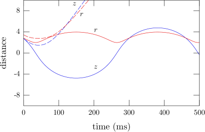
Figure 19: (Color online) Plot of cylindrical coordinates for two orbits near the focus of a dipole trap using the same dipole-trap parameters as in Sec. V, except without gravity. Longitudinal distances ($z$) are in millimeters, and radial distances ($r$) are in ten-micron units. The solid curves show a simulation with $90\%$ of the critical angular momentum required for the dipole-trap focus to become repelling. This trajectory shows an oscillation about the focus that is slowed due to the angular momentum. The dashed curves show the same initial conditions, but with a slightly larger $r$ value and azimuthal velocity, pushing the angular momentum to $110\%$ of the critical value, and show how such a particle can appear to bounce off an attractive potential.

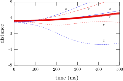
Figure 20: (Color online) Plots of cylindrical coordinates for three orbits in a dipole trap, using the same dipole-trap parameters as in Sec. V, except without gravity. Longitudinal distances ($z$) are in millimeters, and radial distances ($r$) are in ten-micron units. The solid curve shows a slight variation of the predicted saddle-point orbit, with the correct angular momentum but with $q$ slightly below unity. This curve shows the particle oscillating about the saddle-point orbit, but drifting along the $q{=}1$ manifold. The radial restoring force for this orbit in our trap is much stiffer than the longitudinal restoring force, so $r$ oscillates rapidly (resulting in a noncircular orbit). The dashed curve shows the predicted saddle-point orbit, but with $101\%$ of the saddle-point angular momentum; this orbit diverges. The dotted curve shows the predicted saddle-point orbit, but with $99\%$ of the saddle-point angular momentum; this trajectory falls away from the orbit and instead oscillates about the focus.

In this appendix we briefly describe how angular momentum affects atomic motion in a dipole trap formed by a single focused Gaussian beam. The basic effect is that an atom with angular momentum about the trap axis feels an effective force that repels it from the trap focus. A similar effect is experienced by a ball rolling inside a funnel. The tighter confinement toward the center of the funnel (or dipole-trap focus) forces a higher angular velocity in order to conserve angular momentum, which results in an outward push. This effect is often dealt with in classical mechanics textbooks such as Ref. Marion and Thornton (1988) when dealing with central potentials. The angular momentum of a particle in a central potential leads to a centrifugal potential-energy term that repels the particle from the center of the potential.

For this appendix, we will assume we have only the focused Gaussian dipole-trap beam, creating a conservative potential proportional to the local intensity. The potential can thus be written as

$$V{\left(r,z\right)}=-V_{0}\frac{\exp\left({\displaystyle-\frac{2r^{2}}{1+z^{2}}}\right)}{1+z^{2}},$$ (15)

where $r$ is the radial coordinate measured from the trap axis, scaled by the $1/e^{2}$ intensity radius at the focus, and $z$ is the longitudinal coordinate measured from the trap focus, scaled by the Rayleigh length of the beam. We are discussing attractive traps, so $V_{0}$ is assumed to be positive. The quantity in the exponential in Eq. (15) will occur several times in this appendix, so we will abbreviate it as $q^{2}$:

$$q^{2}:=\frac{2r^{2}}{1+z^{2}}.$$ (16)

With this abbreviation, the equations of motion for the cylindrical coordinates become

$$\frac{d^{2}z}{dt^{2}} = -\frac{2V_{0}}{mz_{0}^{2}}z\left(1-q^{2}\right)\frac{\exp\left(-q^{2}\right)}{\left(1+z^{2}\right)^{2}}$$ (17)

$$\frac{d^{2}r}{dt^{2}} = \frac{1}{m^{2}w_{0}^{4}r^{3}}\left[J^{2}-mw_{0}^{2}V_{0}q^{4}\exp\left(-q^{2}\right)\right].$$ (18)

Here $J$ is the conserved angular momentum about the trap axis, and $z_{0}$ and $w_{0}$ are the Rayleigh length and $1/e^{2}$ intensity radius, respectively. Not surprisingly, the focus ($z{=}0$) is a fixed point of the longitudinal motion. What is more surprising is the $(1-q^{2})$ factor. The presence of this factor means that circular orbits with large angular momenta can have significantly smaller accelerations along the trap axis than for one-dimensional motion, even attaining a different sign. We observed experimentally that our trap period was longer than what we would expect from a purely one-dimensional treatment. In simulations we could see that this was partially due to atoms in high-angular-momentum orbits taking a longer time to reach the trap focus. We could also observe the repulsion from the trap center in simulations. This occurs when the energy required for a given angular momentum at the focus is larger than the trap depth. Figure 19 shows simulations of some trajectories with these effects. We took the same simulations used in Sec. V, but with single atoms and initial conditions appropriate for orbits (and no gravity, in order to preserve cylindrical symmetry) near the critical point, illustrating how the focus of the dipole trap changes from attracting to repelling.

This effect helps explain the difference between Figs. 14 and 15. Atoms with some angular momentum have $q>0$, reducing the longitudinal acceleration toward the trap focus in Eq. (17). This is why the simulation in Fig. 15 shows atoms crossing the trap center sooner than the simulation in Fig. 14. Furthermore, because atoms without angular momentum experience more longitudinal acceleration, they are traveling faster along the trap axis when they cross the barrier than their counterparts with angular momentum. We believe this is the main reason why the atoms traverse back and forth across the barrier in Fig. 15 more easily than in Fig. 14—the barrier is effectively higher for atoms that are moving more slowly along the trap axis.

Linear stability analysis of Eqs. (17) and (18) suggests that for $q^{2}=1$, there exist “saddle-point orbits” at some point that is not the trap focus. These orbits require $q^{2}=1$ and $J^{2}=mw_{0}^{2}V_{0}\exp(-1)$, and are stable to perturbations in $q$ but not to perturbations in $J$. They have no linear restoring force along the $q^{2}{=}1$ manifold. We were able to produce simulations that show these strange orbits, but they were so sensitive that we had to remove the effects of gravity from our simulations in order for them to persist. Figure 20 shows one of these orbits and demonstrates how, even with the right conditions, the orbit drifts along the $q^{2}{=}1$ curve. This drift is a result of nonlinear terms in the equations, which dominate because the linear term is zero. Figure 20 also shows how quickly orbits with the wrong angular momentum diverge.

References

- Feynman et al. (1963) R. P. Feynman, R. B. Leighton, and M. Sands, The Feynman Lectures on Physics, vol. 1 (Addison-Wesley, 1963).
- Hänggi and Bartussek (1996) P. Hänggi and R. Bartussek, Lect. Notes Phys. 476, 294 (1996).
- Jülicher et al. (1997) F. Jülicher, A. Ajdari, and J. Prost, Rev. Mod. Phys. 69, 1269 (1997).
- Linke et al. (2005) H. Linke, M. T. Downton, and M. J. Zuckermann, Chaos 15, 026111 (2005).
- Serreli et al. (2007) V. Serreli, C. Lee, E. R. Kay, and D. A. Leight, Nature 445, 523 (2007).
- Mennerat-Robilliard et al. (1999) C. Mennerat-Robilliard, D. Lucas, S. Guibal, J. Tabosa, C. Jurczak, J.-Y. Courtois, and G. Grynberg, Phys. Rev. Lett. 82, 851 (1999).
- Shaw et al. (2007) R. S. Shaw, N. Packard, M. Schröter, and H. L. Swinney, Proc. Natl. Acad. Sci. USA 104, 9580 (2007).
- Raizen et al. (2005) M. G. Raizen, A. M. Dudarev, Q. Niu, and N. J. Fisch, Phys. Rev. Lett. 94, 053003 (2005).
- Ruschhaupt and Muga (2004) A. Ruschhaupt and J. G. Muga, Phys. Rev. A 70, 061604(R) (2004).
- Ruschhaupt and Muga (2006) A. Ruschhaupt and J. G. Muga, Phys. Rev. A 73, 013608 (2006).
- Ruschhaupt et al. (2006a) A. Ruschhaupt, J. G. Muga, and M. G. Raizen, J. Phys. B: At. Mol. Opt. Phys. 39, L133 (2006a).
- Ruschhaupt and Muga (2007) A. Ruschhaupt and J. G. Muga, Phys. Rev. A 76, 013619 (2007).
- Kim and Choi (2005) S. W. Kim and M.-S. Choi, Phys. Rev. Lett. 95, 226802 (2005).
- Dudarev et al. (2005) A. M. Dudarev, M. Marder, Q. Niu, N. J. Fisch, and M. G. Raizen, Europhys. Lett. 70, 761 (2005).
- Ruschhaupt et al. (2006b) A. Ruschhaupt, J. G. Muga, and M. G. Raizen, J. Phys. B: At. Mol. Opt. Phys. 39, 3833 (2006b).
- Price et al. (2007) G. N. Price, S. T. Bannerman, E. Narevicius, and M. G. Raizen, Laser Phys. 17, 965 (2007).
- Ruschhaupt and Muga (2008) A. Ruschhaupt and J. G. Muga, J. Phys. B: At. Mol. Opt. Phys. 41, 205503 (2008).
- Price et al. (2008) G. N. Price, S. T. Bannerman, K. Viering, E. Narevicius, and M. G. Raizen, Phys. Rev. Lett. 100, 093004 (2008).
- Thorn et al. (2008) J. J. Thorn, E. A. Schoene, T. Li, and D. A. Steck, Phys. Rev. Lett. 100, 240407 (2008).
- Bannerman et al. (2009) S. T. Bannerman, G. N. Price, K. Viering, and M. G. Raizen, (submitted for publication) (2009).
- Metcalf and van der Straten (1999) H. J. Metcalf and P. van der Straten, Laser Cooling and Trapping (Springer, 1999).
- Narevicius and Raizen (2009) E. Narevicius and M. G. Raizen, (submitted for publication) (2009).
- Maxwell (1871) J. C. Maxwell, Theory of Heat (Longmans, Green, and Co., New York, 1871).
- Bennett (1987) C. H. Bennett, Scientific American 257, 108 (1987).
- Scully and Scully (2007) R. J. Scully and M. O. Scully, The Demon and the Quantum (Wiley-VCH, Weinheim, 2007).
- Lee et al. (1996) K. I. Lee, J. A. Kim, H. R. Noh, and W. Jhe, Optics Letters 21, 1177 (1996).
- Julienne and Vigué (1991) P. S. Julienne and J. Vigué, Phys. Rev. A 44, 4464 (1991).
- Lett et al. (1995) P. D. Lett, K. Mølmer, S. D. Gensemer, K. Y. N. Tan, A. Kumarakrishnan, C. D. Wallace, and P. L. Gould, J. Phys. B: At. Mol. Opt. Phys. 28, 65 (1995).
- Miller et al. (1993) J. D. Miller, R. A. Cline, and D. J. Heinzen, Phys. Rev. Lett. 71, 2204 (1993).
- Gallagher and Pritchard (1989) A. Gallagher and D. E. Pritchard, Phys. Rev. Lett. 63, 957 (1989).
- Kuppens et al. (2000) S. J. M. Kuppens, K. L. Corwin, K. W. Miller, T. E. Chupp, and C. E. Wieman, Phys. Rev. A 62, 013406 (2000).
- Marion and Thornton (1988) J. B. Marion and S. T. Thornton, Classical Dynamics of Particles and Systems, Third edition (Harcourt Brace Jovanovich, Inc., San Diego, 1988), ISBN 0-15-507640-X.