CMB Polarization and Temperature Power Spectra Estimation using Linear Combination of WMAP 5-year Maps

Abstract

We estimate CMB polarization and temperature power spectra using WMAP $5$-year foreground contaminated maps. The power spectrum is estimated by using a model independent method, which does not utilize directly the diffuse foreground templates nor the detector noise model. The method essentially consists of two steps, (i) removal of diffuse foregrounds contamination by making linear combination of individual maps in harmonic space and (ii) cross-correlation of foreground cleaned maps to minimize detector noise bias. For temperature power spectrum we also estimate and subtract residual unresolved point source contamination in the cross-power spectrum using the point source model provided by the WMAP science team. Our $TT$, $TE$ and $EE$ power spectra are in good agreement with the published results of the WMAP science team. The error bars on the polarization power spectra, however, turn out to be smaller in comparison to what is obtained by the WMAP science team. We perform detailed numerical simulations to test for bias in our procedure. We find that the bias is small in all cases. A negative bias at low $l$ in $TT$ power spectrum has been pointed in an earlier publication. We find that the bias corrected quadrupole power ($l(l+1)C_{l}/2\pi)$ is $532$ $\mu K^{2}$, approximately $2.5$ times the estimate ($213.4$ $\mu K^{2}$) made by the WMAP team.

1 Introduction

The anisotropies of the Cosmic Microwave Background (CMB) radiation are the most important evidence behind the tiny fluctuations that are generated by the inflationary paradigm of the Big-Bang cosmology (Starobinsky (1982); Guth & Pi (1982); Bardeen et al. (1983)). One can determine cosmological parameters precisely by measuring these anisotropies (Jungman et al. (1996b, a); Bond et al. (1997); Zaldarriaga et al. (1997)). These anisotropies possess a certain degree of linear polarization due to the quadrupolar temperature pattern seen by the moving electrons in the primordial plasma (Rees (1968); Basko & Polnarev (1980)). Recently, the WMAP satellite has mapped the total intensity and polarization of the CMB anisotropies over the full sky in its $5$ frequency bands from $23$ GHz to $94$ GHZ with unprecedented resolution and sensitivity (Bennett et al. (2003a, b); Page et al. (2007); Kogut et al. (2007); Hinshaw et al. (2008)). The polarization power spectrum acts as a complement to the temperature power spectrum. It leads to better constraints on the cosmological parameters and is also useful to break degeneracies among certain cosmological parameters, e.g. epoch of reionization and scalar to tensor ratio (Kinney (1998)). Furthermore it has been argued that CMB polarization may serve as a direct probe of inflation (Spergel & Zaldarriaga (1997)), can test if the parity symmetry is preserved on the cosmological scales (Lue et al. (1999); Komatsu et al. (2008)), can provide information about the epoch when the first stars begin to form (Crittenden et al. (1993); Ng & Ng (1995)) and provide a measure of the gravity waves that are generated by inflation (Harari & Zaldarriaga (1993); Crittenden et al. (1995); Kamionkowski & Kosowsky (1998)). The WMAP team have produced their temperature and polarization power spectrum based upon the foreground cleaned maps which are obtained using prior models of the synchrotron, dust and free-free components (Kogut et al. (2007); Page et al. (2007)). Though this method allows one to use all the available information about the foreground components it is also a very important scientific task to perform an independent analysis of the data by techniques which do not rely upon explicit foreground modeling.

A multipole based approach for foreground removal was first proposed by Tegmark & Efstathiou (1996) and was implemented on the WMAP data by Tegmark et al. (2003). Later, Saha et al. (2006, 2008); Souradeep et al. (2006) extended this method to extract the temperature anisotropy power spectrum of the Cosmic Microwave Background (CMB) radiation from the raw WMAP data. The power spectrum is obtained by forming several cleaned maps using subsets of the available maps and thereafter cross-correlating the resulting maps. This Internal Power Spectrum Estimation (IPSE) method utilizes CMB data as the only input without making any explicit modeling of the diffuse galactic foreground components or detector noise bias. The foreground components are removed using the fact that in thermodynamic temperature unit, the CMB signal is predicted to be independent of frequency since it follows a black-body spectrum (Mather et al. (1994); Fixsen et al. (1996)), while the foreground components are frequency dependent. The detector noise bias is removed by cross-correlating different foreground cleaned maps obtained by using independent detector subsets. This substantially removes the noise bias since, to a good approximation, WMAP detector noise is uncorrelated for two different detectors (Jarosik et al. (2003, 2007)). The final power spectra (Saha et al. (2006, 2008)) obtained by IPSE agrees well with the results published by the WMAP science team. Thus the method serves as an independent technique to verify the main power spectrum result obtained by the WMAP science team starting from the stage of diffuse foreground components removal. The method has several advantages. First, the foreground components removal method is entirely independent of the foreground template models. Therefore the foreground cleaned maps are not susceptible to systematic errors that might arise in template based methods due to incorrect template modeling. Second, the cleaned power spectrum can be studied analytically in the special case of full sky one iteration foreground cleaning (Saha et al. (2008)). This allows us to quantify and understand the statistical properties of the residuals in the cleaned power spectrum. This may be very useful in the case of noisy data or when the total number of available frequency bands are less than the total number of independent parameters required for satisfactory modeling of all dominant underlying components. A detailed analytical study of the bias in the cleaned power spectrum is presented in Saha et al. (2008). Third, it is possible to obtain a model independent estimate of the map and power spectrum of the total foreground emission at each of the frequency bands (Ghosh et al. (2009)).

In the present paper we extract CMB polarization $EE$, $TE$ as well as the $TT$ power spectra using the WMAP $5$-year foreground and detector noise contaminated maps as input to IPSE – our combined foreground removal and power spectrum estimation procedure. Since the CMB polarization signal is weak the polarized maps published by the WMAP science team are dominated by the foreground components and detector noise. This seriously limits the accuracy with which the polarized CMB power spectrum can be extracted. However, since our method does not use any template model to remove foreground components we argue that our power spectrum is free from systematic effects that might arise due to incorrect modeling of polarized (and temperature) foreground templates.

The error bars as well as the bias in the extracted polarization power spectrum are estimated by numerical Monte Carlo simulations. Here we make use of explicit foreground and detector noise models. In the case of temperature power spectrum a similar analysis reveals the presence of a negative bias at low multipoles (Saha et al. (2008)). The bias corrected temperature spectra explains almost all of the low power observed in case of quadrupole. In this case it is also possible to analytically obtain an estimate of the bias in some special cases.

Alternate approaches of CMB power spectrum estimation have been studied by several authors, e.g., using foreground cleaned maps provided by the WMAP science team (Fosalba & Szapudi (2004); Patanchon et al. (2005); Eriksen et al. (2007a, b)), as well as using uncleaned maps where some models of foregrounds and (or) detector noise are necessary (Eriksen et al. (2008b, a)). Other approaches for foreground cleaning, using needlet coefficients (Delabrouille et al. (2009)) and harmonic variance minimization (Kim et al. (2008a, b)) have also been proposed.

The organization of our paper is as follows. We describe the methodology of power spectrum estimation in Section 2. We present the power spectrum results along with their covariance structure in Section 3. Finally, we conclude in Section 4.

2 Method

The basic procedure for extracting the temperature power spectrum is described in Saha et al. (2006) and Saha et al. (2008). Here we generalize this to include polarization. The basic maps for the case of polarization are available in terms of the Stokes parameters $Q$ and $U$. Since these are coordinate dependent quantities it is more convenient to work with the coordinate independent $E$ and $B$ modes (Zaldarriaga & Seljak (1997); Seljak & Zaldarriaga (1997); Kamionkowski et al. (1997)). Another problem with using $Q$ and $U$ maps is that the $E$ and $B$ modes mix with one another when one applies a sky mask (Jaffe et al. (2000); Tegmark & de Oliveira-Costa (2001); Bunn et al. (2003); Smith & Zaldarriaga (2007)) to remove heavily contaminated Galactic regions. This demands an extra data processing step to isolate the actual CMB $E$ and $B$ mode power spectra from their mixture. To avoid this problem we start by converting full sky $Q$ and $U$ maps to full sky $E$ and $B$ maps and apply mask whenever required on the resultant maps. This is similar to what is proposed in Betoule et al. (2009) for estimating $r=T/S$ for the Planck satellite mission and the Experimental Probe of Inflationary Cosmology (EPIC). To obtain the $E$ and $B$ maps we first expand the full sky spin $\pm 2$ fields $(Q\pm iU)$ in terms of spin-2 spherical harmonics $\;{}_{\pm 2}Y_{lm}(\hat{n})$

$$(Q+iU)(\hat{n})=\sum_{lm}a_{2,lm}\;{}_{2}Y_{lm}(\hat{n})$$

$$(Q-iU)(\hat{n})=\sum_{lm}a_{-2,lm}\;{}_{-2}Y_{lm}(\hat{n})$$ (1)

Since both $Q$ and $U$ are real, one can show that the expansion coefficients obey $a^{*}_{-2,lm}=a_{2,l-m}$. The spin-0 $E$ and $B$ are now obtained by the usual spherical harmonic transform,

$$E(\hat{n})=\sum_{l\geq 2,|m|\leq l}a_{lm}^{E}Y_{lm}(\hat{n})$$

$$B(\hat{n})=\sum_{l\geq 2,|m|\leq l}a_{lm}^{B}Y_{lm}(\hat{n})$$ (2)

where

$$a_{lm}^{E}=\frac{1}{2}(a_{2,lm}+a_{-2,lm})$$

$$a_{lm}^{B}=\frac{1}{2i}(a_{2,lm}-a_{-2,lm})$$ (3)

This gives us $10$ different full sky maps for each of the $E$ and $B$ fields corresponding to the $10$ WMAP Differencing Assemblies (DAs). The 10 DAs are labeled as K, Ka, Q1, Q2, V1, V2, W1, W2, W3, W4 corresponding to the five different frequency channels K, Ka, Q, V and W. We note that the bands Q, V and W have 2, 2, 4 DAs respectively.

We first eliminate the highly contaminated Galactic plane from all the $10$ DA maps using P06 mask (Page et al. (2007)). This procedure is slightly different from that described in Saha et al. (2006, 2008). In the latter case the authors cleaned the entire unmasked sky in nine iterations and also produced a full sky foreground cleaned temperature maps. However to eliminate potential residual foreground contamination arising from the Galactic plane the KQ85 mask (Gold et al. (2008)) is applied before computing the power spectrum. In the present work, we apply the mask right at the beginning since we are interested in extracting only the power spectrum. To cross-check our one iteration method we also divide the EE maps in several parts and then perform foreground removal in the iterative approach. We find that, the final power spectrum of this method is similar to the one iteration case.

We select different possible linear combinations of $4$ maps out of the available DAs as described below. The entire set of linear combinations are listed in Table 1. Each of these linear combinations independently lead to a clean map.

The cleaning is accomplished independently for each $l$, by linearly combining these maps with weights, $\hat{w}_{l}^{a}$, such that the spherical harmonic components of the cleaned map are given by,

$$a_{lm}^{\rm Clean}=\sum_{a=1}^{n_{c}}\hat{w}_{l}^{a}\frac{a_{lm}^{a}}{B_{l}^{a}}\,.$$ (4)

Here $n_{c}$ is the total number of maps used for cleaning. In the present case of $4$ channel cleaning, $n_{c}=4$. The factor $B_{l}^{a}$ is the circularized beam transform function for the frequency band $a$ (Hill et al. (2008)). The weights $\hat{w}_{l}^{a}$ are chosen so as to minimize the total power subject to the constraint

$${\hat{\textbf{W}}}_{l}{\textbf{e}}_{0}={\textbf{e}}^{T}_{0}{\hat{\textbf{W}}}^{T}_{l}=1\,,$$ (5)

where ${\textbf{e}}_{0}$ is a column vector with unit elements

$${\textbf{e}}_{0}=\left(\begin{array}[]{c}1\\ ..\\ ..\\ 1\end{array}\right)\,,$$ (6)

and $\hat{\textbf{W}}_{l}$ is the row vector $(\hat{w}_{l}^{1},\hat{w}_{l}^{2},..,\hat{w}_{l}^{n_{c}})$. This constraint is required so as to preserve the CMB signal. The weights are obtained using the empirical covariance matrix, $\hat{\textbf{C}}_{l}$, by the relationship, (Saha et al. (2006, 2008); Tegmark et al. (2003); Tegmark & Efstathiou (1996); Eriksen et al. (2004); Delabrouille & Cardoso (2009))

$$\hat{\textbf{W}}_{l}=\frac{{\textbf{e}}^{T}_{0}(\hat{\textbf{C}}_{l})^{-1}}{{\textbf{e}}^{T}_{0}(\hat{\textbf{C}}_{l})^{-1}{\textbf{e}}_{0}}\,.$$ (7)

We label the resulting cleaned maps as Ci and CAi where ${\textbf{i}}=1,2,...,24$. Here the maps Ci use the DAs K along with possible combinations of DAs from the bands Q, V and W. Similarly the maps CAi include Ka instead of K. The entire nomenclature is listed in Table 1. In the case of the W band we average over two DAs before we start the foreground cleaning. Hence in Table 1 the notation W12, for example, refers to the average of the DAs W1 and W2. This averaging is not essential to the procedure and one may also directly use the original WMAP DAs. However averaging leads to a reduced detector noise in each cleaned map.

K + Q1 + V1 + W12 = C1	Ka + Q1 + V1 + W12 = CA1
K + Q1 + V1 + W13 = C2	Ka + Q1 + V1 + W13 = CA2
K + Q1 + V1 + W14 = C3	Ka + Q1 + V1 + W14 = CA3
K + Q1 + V1 + W23 = C4	Ka + Q1 + V1 + W23 = CA4
K + Q1 + V1 + W24 = C5	Ka + Q1 + V1 + W24 = CA5
K + Q1 + V1 + W34 = C6	Ka + Q1 + V1 + W34 = CA6
K + Q2 + V2 + W12 = C7	Ka + Q2 + V2 + W12 = CA7
K + Q2 + V2 + W13 = C8	Ka + Q2 + V2 + W13 = CA8
K + Q2 + V2 + W14 = C9	Ka + Q2 + V2 + W14 = CA9
K + Q2 + V2 + W23 = C10	Ka + Q2 + V2 + W23 = CA10
K + Q2 + V2 + W24 = C11	Ka + Q2 + V2 + W24 = CA11
K + Q2 + V2 + W34 = C12	Ka + Q2 + V2 + W34 = CA12
K + Q1 + V2 + W12 = C13	Ka + Q1 + V2 + W12 = CA13
K + Q1 + V2 + W13 = C14	Ka + Q1 + V2 + W13 = CA14
K + Q1 + V2 + W14 = C15	Ka + Q1 + V2 + W14 = CA15
K + Q1 + V2 + W23 = C16	Ka + Q1 + V2 + W23 = CA16
K + Q1 + V2 + W24 = C17	Ka + Q1 + V2 + W24 = CA17
K + Q1 + V2 + W34 = C18	Ka + Q1 + V2 + W34 = CA18
K + Q2 + V1 + W12 = C19	Ka + Q2 + V1 + W12 = CA19
K + Q2 + V1 + W13 = C20	Ka + Q2 + V1 + W13 = CA20
K + Q2 + V1 + W14 = C21	Ka + Q2 + V1 + W14 = CA21
K + Q2 + V1 + W23 = C22	Ka + Q2 + V1 + W23 = CA22
K + Q2 + V1 + W24 = C23	Ka + Q2 + V1 + W24 = CA23
K + Q2 + V1 + W34 = C24	Ka + Q2 + V1 + W34 = CA24

Table 1: List of the different combination of the DA maps, used to obtain the final 48 cleaned maps, denoted by $C{\textbf{i}}$ and $CA{\textbf{i}}$ where i = 1, 2, …, 24.

After obtaining the $48$ cleaned maps we cross-correlate them in selected combinations in order to reduce the contribution due to detector noise. We cross-correlate all pairs of maps such that the two cleaned maps in each pair are formed by distinct DAs. This gives us $24$ cross-correlated power spectra on the masked sky. All the possible cross-correlations are listed in Table 2.

C1 $\otimes$ CA12	C2 $\otimes$ CA11	C3 $\otimes$ CA10	C4 $\otimes$ CA9	C5 $\otimes$ CA8	C6 $\otimes$ CA7
C7 $\otimes$ CA6	C8 $\otimes$ CA5	C9 $\otimes$ CA4	C10$\otimes$ CA3	C11$\otimes$ CA2	C12$\otimes$ CA1
C13$\otimes$ CA24	C14$\otimes$ CA23	C15$\otimes$ CA22	C16$\otimes$ CA21	C17$\otimes$ CA20	C18$\otimes$ CA19
C19$\otimes$ CA18	C20$\otimes$ CA17	C21$\otimes$ CA16	C22$\otimes$ CA15	C23$\otimes$ CA14	C24$\otimes$ CA13

Table 2: List of all the $24$ cross-power spectra using the $48$ cleaned maps, C1, C2,…, C24 and CA1, CA2,…, CA24.

We convert each of the $24$ masked sky power spectra into full sky estimates of the underlying CMB power spectrum using the mode-mode coupling matrix corresponding to the P06 mask following the MASTER approach (Hivon et al. (2002); Hinshaw et al. (2003); Tristram et al. (2005)). We then remove beam and pixel effects from each of these $24$ full sky power spectra. Our final $EE$ power spectrum is simply an uniform average of these $24$ cross-spectra. We rely upon Monte Carlo simulations to compute the error bars as well as possible bias in the extracted power spectrum.

The neighboring multipoles in the power spectrum become coupled since the spherical harmonics lose orthogonality on a masked sky. Hence, to obtain full information about the two-point correlation function of the resulting power spectrum one needs to construct the covariance matrix,

$$\left<\Delta C_{l}\Delta C_{l^{\prime}}\right>=\left<(C_{l}-\left<C_{l}\right>)(C_{l^{\prime}}-\left<C_{l^{\prime}}\right>)\right>\ ,$$

We compute the covariance matrix by Monte Carlo simulations. The correlations can be minimized by suitably binning the power spectrum. We use a binning identical to that used by the WMAP team. Let $C_{\alpha}$ denote the binned power spectrum. Then the covariance matrix of the binned spectrum is obtained as

$$\left<\Delta C_{\alpha}\Delta C_{\alpha^{\prime}}\right>=\left<(C_{\alpha}-\left<C_{\alpha}\right>)(C_{\alpha^{\prime}}-\left<C_{\alpha^{\prime}}\right>)\right>\ .$$

The standard deviation obtained from the diagonal elements of the binned covariance matrix gives the error-bars on the binned final spectrum. Since the cosmic variance of the CMB power spectrum decays as $\sim 1/(2l+1)$, the diagonal terms in the above correlation matrix decay with increasing multipoles. For a visual comparison of correlation between different bins we define a correlation matrix, $C_{\alpha\alpha^{\prime}}$, of the binned power spectrum, where,

$$C_{\alpha\alpha^{\prime}}=\frac{\left<\Delta C_{\alpha}\Delta C_{\alpha^{\prime}}\right>}{\sqrt{\left<(\Delta C_{\alpha})^{2}\right>\left<(\Delta C_{\alpha^{\prime}})^{2}\right>}}\,.$$ (8)

All the elements of this matrix are bound to lie between $[-1,1]$.

3 Results

3.1 Temperature Power Spectrum

The temperature power spectrum for $5$-year WMAP data is obtained using the same procedure as described in Saha et al. (2008)). The entire sky is divided into $9$ regions depending on the level of foreground contamination. The whole cleaning is done with the iterative method, starting from the dirtiest region.

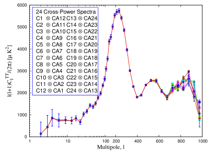
Figure 1: The 24, binned, $TT$ cross power spectra obtained by using the WMAP 5 year data. All the different combinations of cleaned maps used are shown in the box. The average power spectrum along with error bars (blue points) is also shown. The red line joins the individual binned averages.

All the 24 cross power spectra for temperature anisotropy are shown in Fig. 1. We form an uniform average power spectrum by averaging over these 24 cross power spectra. While obtaining the cleaned power spectrum we use the KQ85 mask to remove the residual foreground contamination near the Galactic plane.

Even after applying the KQ85 mask which also removes a circular region around each of the known point sources, residual unresolved point sources cause a significant contamination in this power spectrum. There have been several attempts to measure unresolved point source contamination in the CMB maps ( Tegmark & de Oliveira-Costa (1998); Komatsu et al. (2003); Huffenberger et al. (2006)). We estimate unresolved point source contamination in our final power spectrum using the model presented by Nolta et al. (2008) following an approach similar to that in Saha et al. (2006, 2008).

We compute the bias in the extracted spectrum by performing $150$ Monte Carlo simulations. First we generate synchrotron, free-free and thermal dust maps corresponding to different WMAP frequencies using the Planck Sky Model (PSM). Although several options are available in the PSM to generate galactic emission (e.g. with or without spinning dust, with or without small scales added), the largest scales in temperature are strongly constrained by observation, and the impact of the choice of a particular model is not a major source of uncertainty. In our simulations, we use a single set of galactic emission maps, which comprise a two-component dust model based on SFD model 7, synchrotron map with varying spectral index in agreement with the first year WMAP data, and free-free emission with fixed spectral index, obtained from an H-alpha template corrected for galactic dust extinction. The exact polarisation properties of the galactic foregrounds, in particular that of dust emission, are poorly constrained by observations. For the present work, we use version 1.6.4 of the PSM (see Betoule et al. (2009) for details about the polarised galactic emission). In the next step we randomly generate CMB maps assuming the standard $LCDM$ model (Spergel et al. (2003)). Each random realization of the CMB map is then added to the combined mixture of all three foreground components corresponding to the $5$ WMAP frequencies. Using the $5$ year beam transform functions for different DAs provided by the WMAP science team, we transform the $5$ resulting maps into $10$ maps. Each map at this step has a resolution appropriate for the corresponding DA. We then generate random noise maps corresponding to each detector. The random noise maps are generated by sampling a Gaussian distribution with unit variance and then multiplying each Gaussian variable by $\sigma_{0}/\sqrt{N_{p}}$, where $\sigma_{0}$ is the noise per observation (Hinshaw et al. (2008)) and $N_{p}$ the effective number of observations at each pixel. The values of $\sigma_{0}$ depend on the DA, with the smallest value for the K band DA and largest for the W band DAs. Finally the noise maps are added to the CMB plus foreground maps for different DAs. These maps with CMB signal, detector noise and foreground are then passed through the same power spectrum estimation method as in the case of observed data. The mean of the $150$ extracted spectra gives the final simulated power spectrum. The standard deviation of the $150$ simulations gives the error. The difference between the simulated power and the input $LCDM$ power gives a measure of the bias in our method. This bias is subtracted from the extracted power spectrum in order to get the final result.

The precise magnitude of the bias depends on the theoretical model with which we compare our extracted power spectrum. In other words, before we compare our extracted power to a theoretical model, we must correct for bias using the corresponding model power spectrum. Here we use the WMAP best fit $LCDM$ model to compute the theoretical power spectrum.

The final temperature power spectrum using the Internal Power Spectrum Estimation (IPSE) method, after correcting for bias, is shown in Fig. 2. We find that it is in good agreement with the WMAP best fit $LCDM$ model. The simulation results are also shown in Fig. 2. After bias correction we find the quadrupole power ($l(l+1)C_{l}/2\pi$) equal to $532$ $\mu K^{2}$ compared to the value of $213.4$ $\mu K^{2}$ estimated by the WMAP science team. The quadrupole extracted from IPSE is, therefore, in much better agreement with the theoretical model.

The correlation matrix, Eq. 8, for temperature power spectrum is shown in Fig. 3. We find, as expected, that the off diagonal matrix elements are negligible compared to the diagonal elements.

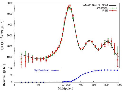
Figure 2: The final, binned, $TT$ power spectrum using IPSE (red dots) along with error bars for the 5 year WMAP data, after subtracting the bias extracted using simulations. The error bars are also obtained from simulations. The WMAP $LCDM$ best fit model (black line) and the simulation results (green crosses) are shown for comparison. The bottom panel shows the correction made for residual power from unresolved point source contamination.

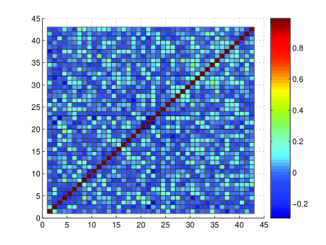
Figure 3: The correlation matrix elements, $C_{\alpha\alpha^{\prime}}$, defined in Eq. 8, for the temperature power spectrum, plotted with respect to the bin indices $\alpha,\alpha^{\prime}$.

3.2 The $TE$ power spectrum

The WMAP polarization CMB maps are cleaned using a single iteration rather than the nine iteration procedure followed for temperature anisotropy. We apply the P06 mask right in the beginning. The mask removes 27% of the entire sky region near the galactic plane. The cleaning algorithm is applied only to regions outside the P06 mask. Hence we make no attempt to produce a full sky cleaned polarization map.

The error bars plotted in the $TE$ power spectrum are obtained by Monte Carlo simulations. We generate $150$ random samples of data using the $LCDM$ model (Spergel et al. (2003)) and simulated foregrounds and detector noise. First we generate the synchrotron and thermal dust polarized foreground maps corresponding to different frequencies in terms of Q and U maps using the PSM version 1.6.4. The free-free emission is not polarized and hence not included. The anomalous dust emission is also assumed to be unpolarized and thus is not included either. Using the HEALPix command synfast we generate random realization of CMB polarization maps in terms of Q and U maps. The random CMB realization and foreground maps are smoothed by the beam functions corresponding to ten different DAs. We next obtain E-mode polarization maps from these Q and U maps. Then we generate random noise maps for each DA in terms of Stokes parameters Q and U using Cholesky decomposition technique for generating correlated Gaussian random variables using the WMAP supplied $2\times 2$ QU intra-pixel noise covariance matrices. These Q and U noise maps are converted to E mode noise maps. The final E-maps including detector noise, foregrounds and CMB signal are passed through the same cleaning pipeline as the observed polarization data. In order to minimize the correlation among neighboring $l$ modes, the final power spectrum is binned in the same way as the WMAP 5 year result. Here also the standard deviation obtained from the diagonal elements of the binned covariance matrix is used as the error bars on the binned final spectrum extracted from the WMAP data.

The extracted $TE$ power spectrum along with the WMAP results and the best fit $LCDM$ model is shown in Fig. 4. The binned $TE$ power spectrum, using the same binning scheme as used by the WMAP team, is shown in Fig. 5. The error bars are computed by simulations. The simulation results are shown in Fig. 6. We find that the bias is small for all the bins. Only at small $l$, $l<10$, do we find a noticeable negative bias. For larger $l$, the bias is practically negligible. The bias corrected $TE$ power spectrum is shown in Fig. 7. The spectrum obtained by the WMAP science team as well as their best fit $LCDM$ model is also shown. We find good agreement with the WMAP result. However we obtain slightly smaller error bars. We discuss the possible cause for this in the next subsection. The correlation matrix elements, Eq. 8, are shown in Fig. 8. Here also we see that they are dominated by diagonal elements.

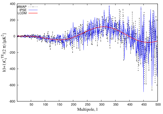
Figure 4: The cleaned $TE$ power spectrum using IPSE (solid blue line) along with WMAP result (dashed black line). The WMAP best fit $LCDM$ power spectrum (thick solid red line) is shown for comparison.

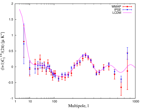
Figure 5: The final binned $TE$ power spectrum using IPSE (blue diamonds) along with error bars, compared with the WMAP results (red dots). The WMAP best fit $LCDM$ result (solid pink line) is also shown.

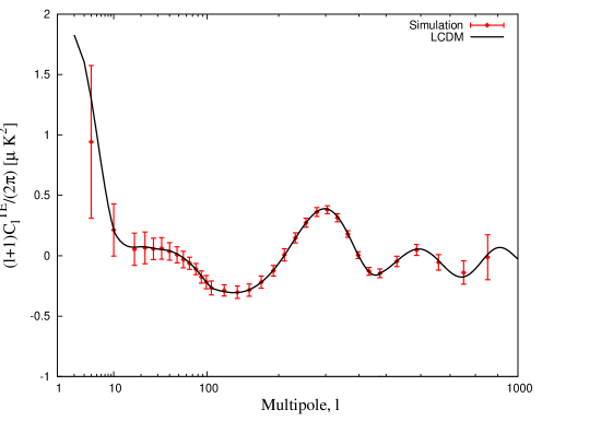
Figure 6: The binned $TE$ power spectrum, along with error bars, obtained from simulations (red dots). The input $LCDM$ model (solid black line) is also shown.

Figure 7: The bias corrected, binned $TE$ power spectrum using IPSE (blue diamonds) along with error bars, compared with the WMAP results (red dots). The WMAP best fit $LCDM$ power spectrum (solid pink line) is also shown.

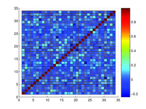
Figure 8: The covariance matrix elements, $C_{\alpha\alpha^{\prime}}$, defined in Eq. 8, for the $TE$ power spectrum plotted with respect to the bin indices $\alpha,\alpha^{\prime}$.

3.3 The $EE$ power spectrum

The binned $EE$ power spectrum, using the WMAP binning procedure, along with the simulation results, is shown in Fig. 9 for the 5 year data. In this figure we also show the $EE$ power spectrum extracted by the WMAP team along with the WMAP best fit $LCDM$ model. In Fig. 9 we follow exactly the WMAP binning procedure and consider only the multipoles $l\geq 50$. The results for low multipoles $l<50$ are shown separately. We find that our extracted power spectrum is in good agreement with that obtained by the WMAP team but with significantly smaller error bars. Furthermore the binned simulated power spectrum is found to be close to the input $LCDM$ power over the entire multipole range. Only at small $l$ do we find a significant positive bias. For the remaining multipoles the simulation results match the input power within error bars. The bias corrected power spectrum is shown in Fig. 10. We see that the bias corrected spectrum is in reasonable agreement with the best fit $LCDM$ model. The correlation matrix elements are shown in Fig. 11. We again find that the correlation matrix is dominated by diagonal matrix elements.

Our extracted power spectrum along with the simulation results for low $l$ ($l\leq 50$) are shown in Fig. 12. The WMAP power spectrum as well as their best fit $LCDM$ model is also shown. Here we have chosen the binning that was used by the WMAP team for the TE power spectrum. The bias corrected power spectrum is shown in Fig. 13.

Since the power spectrum estimation methodology described in this work is fundamentally different from WMAP team’s approach we should not expect both methods to produce identical error-bars on the derived power spectra, although the power spectra themselves, obtained by using the two methods, are in reasonable agreement with each other. We find that our error-bars on the polarization power spectra are smaller compared to those obtained by the WMAP science team. This effect could be explained by noting that we use more detector maps for polarization power spectrum estimation than WMAP science team. Using more detectors increases the signal to noise ratio of the cleaned map by decreasing the effective noise level. The reduced noise level leads to lower error-bar on our polarization power spectra. Furthermore, in the case of noisy polarization data the weights tend to be inversely proportional to the noise. Due to this inverse noise weighting each cleaned map has lesser noise in comparison to the least noisy K or Ka band maps. This may be another reason for smaller error bars in the case of polarization power spectrum.

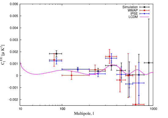
Figure 9: The CMB polarization $EE$ power spectrum using IPSE (blue diamonds) along with error bars, compared with the WMAP result (red dots). The WMAP best fit $LCDM$ power spectrum (pink solid line) and the simulation results (black crosses) are also shown.

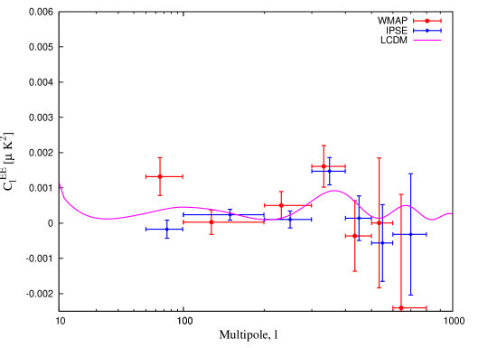
Figure 10: The CMB polarization $EE$ power spectrum using IPSE (blue diamonds) along with error bars, after correcting for bias. The WMAP result (red dots) and the theoretical $LCDM$ spectrum (pink solid line) are shown for comparison.

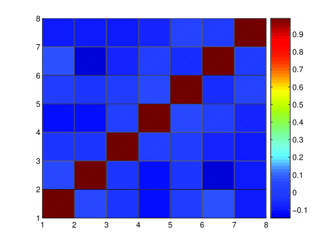
Figure 11: The correlation matrix elements, $C_{\alpha,\alpha^{\prime}}$, defined in Eq. 8, for the $EE$ power spectrum plotted with respect to the bin indices $\alpha,\alpha^{\prime}$.

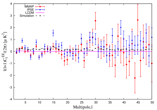
Figure 12: The binned $EE$ power spectrum using IPSE (blue diamonds) at low-$l$ along with the results by the WMAP science team (red dots). The theoretical $LCDM$ spectrum (solid pink line) and the ensemble averaged $EE$ power spectrum from simulated data (dashed black line) are also shown.

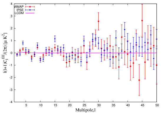
Figure 13: The bias corrected $EE$ power spectrum using IPSE (blue diamonds) at low-$l$ compared with the WMAP results (red dots). The WMAP best fit $LCDM$ power spectrum (pink line) is also shown.

4 Conclusion

We have used a model independent method to estimate the CMB temperature and polarization power spectrum using WMAP $5$-year data. The method is based on the assumption that the CMB signal is independent of frequency in thermodynamic temperature unit. Since the foregrounds are frequency dependent in this unit, it is possible to minimize the foreground power by making a linear combination of CMB maps with a suitable choice of weights. For foreground minimization we use the CMB maps in harmonic space. For the case of polarization, the raw full-sky $Q$ and $U$ maps are first converted to $E$ and $B$ maps to avoid any mixing of E and B modes. The total number of maps available for each field for WMAP data is ten, corresponding to the ten DAs. We create several cleaned maps by choosing different subsets of ten DAs, such that each set contains only four DAs. The detector noise power is minimized by cross correlating cleaned maps obtained from distinct DAs. This leads to a considerable reduction of the detector noise power since, to a good approximation, noise is uncorrelated among different detectors.

By utilizing all the ten WMAP DA maps to estimate the polarization power spectra, we are able to provide more stringent constraints on the spectra in comparison to that obtained by the WMAP science team. We find that the error-bars on our $TE$ and $EE$ power spectra are smaller than those obtained by the WMAP science team on all angular scales. Another possible reason for why we get smaller error bars in the case of polarization power spectra is that in a noisy data the weights tend to combine the maps in inverse noise weighted manner. This results in each cleaned map having lesser noise than the least noisy K or Ka band maps.

In the case of $TT$ power spectrum we find that our procedure does not remove all the unresolved point source contamination. This contamination is significant at small angular scales where the detector noise is also very large. Hence here our internal cleaning is not very efficient. The residual unresolved point source contamination is removed by using the WMAP point source model, as described in detail in Saha et al. (2006, 2008).

We have performed detailed simulations of the $TT$, $TE$, $EE$ power spectrum, using the WMAP best fit $LCDM$ model, along with foreground and detector noise models, in order to determine if there exists any bias in the extracted power. In all cases the bias is found to be small for the entire multipole range. The extracted power, with or without bias correction, is found to be in good agreement with the WMAP results. In Saha et al. (2008) the authors noticed a negative bias at low $l$ in the $TT$ power spectrum. The negative bias arises due to a chance correlation between the CMB and the foregrounds. After correcting for the negative bias, we find that the quadrupole for the WMAP 5 year data shows much better agreement with the $LCDM$ model, in comparison to the result obtained by the WMAP science team. Excluding $l=2$, we find negligible bias at all multipoles except at very large $l$ values, where we find a small positive bias. For the case of $TE$ power spectrum we also find a small negative bias at low $l$, $l<10$. For larger $l$ values the bias is negligible. For $EE$ power spectrum also the bias is found to be small compared to the corresponding error bars. A significant positive bias is found only at low $l$.

To summarize, we have performed a completely independent reanalysis of WMAP $5$ years temperature and polarization data. Our procedure uses primarily the CMB data. Hence it is free from any bias that might result from the inadequacies and inaccuracies of the foreground modeling. The foreground templates and detector noise modeling is utilized only for the purpose of bias analysis and error estimation. The bias is found to be small for all the spectra over the entire multipole range. Our results verify the basic power spectra results obtained by the WMAP Science team. We expect that the method will be very useful for analyzing data from future CMB probes such as Planck.

5 Acknowledgments

We acknowledge the use of Legacy Archive for Microwave Background Data Analysis. Some of the results of this work are derived using the publicly available HEALPIx package (Górski et al. (2005)). (The HEALPIX distribution is publicly available from the website http://healpix.jpl.nasa.gov.) We acknowledge the use of the Planck Sky Model, developed by the Component Separation Working Group (WG2) of the Planck Collaboration. Pramoda K. Samal acknowledges CSIR, India for financial support under the research grant CSIR-SRF- 9/92(340)/2004-EMR-I. A portion of the research described in this paper was carried out at the Jet Propulsion Laboratory, California Institute of Technology, under a contract with the National Aeronautics and Space Administration.

References

- Bardeen et al. (1983) Bardeen, J. M., Steinhardt, P. J., & Turner, M. S. 1983, Phys. Rev. D, 28, 679
- Basko & Polnarev (1980) Basko, M. M., & Polnarev, A. G. 1980, Soviet Astronomy, 24, 268
- Bennett et al. (2003a) Bennett, C. L. et al. 2003a, Astrophys. J. Series, 148, 1, arXiv:astro-ph/0302207
- Bennett et al. (2003b) ——. 2003b, Astrophys. J. Series, 148, 97, arXiv:astro-ph/0302208
- Betoule et al. (2009) Betoule, M., Pierpaoli, E., Delabrouille, J., Le Jeune, M., & Cardoso, J.-F. 2009, ArXiv e-prints, 0901.1056
- Bond et al. (1997) Bond, J. R., Efstathiou, G., & Tegmark, M. 1997, Mon. Not. R. Astron. Soc., 291, L33, arXiv:astro-ph/9702100
- Bunn et al. (2003) Bunn, E. F., Zaldarriaga, M., Tegmark, M., & de Oliveira-Costa, A. 2003, Phys. Rev. D, 67, 023501
- Crittenden et al. (1993) Crittenden, R., Davis, R. L., & Steinhardt, P. J. 1993, Astrophys. J. Lett., 417, L13+, arXiv:astro-ph/9306027
- Crittenden et al. (1995) Crittenden, R. G., Coulson, D., & Turok, N. G. 1995, Phys. Rev. D, 52, 5402, arXiv:astro-ph/9411107
- Delabrouille & Cardoso (2009) Delabrouille, J., & Cardoso, J.-F. 2009, Data Analysis in Cosmology, Lecture notes in physics 665, eds Springer, Vicent Martinez et al. eds, 159, arXiv:astro-ph/0702198
- Delabrouille et al. (2009) Delabrouille, J., Cardoso, J.-F., Le Jeune, M., Betoule, M., Fay, G., & Guilloux, F. 2009, Astronomy and Astrophysics, 493, 835, arXiv:astro-ph/0807.0773
- Eriksen et al. (2004) Eriksen, H. K., Banday, A. J., Górski, K. M., & Lilje, P. B. 2004, Astrophys. J., 612, 633, arXiv:astro-ph/0403098
- Eriksen et al. (2008a) Eriksen, H. K., Dickinson, C., Jewell, J. B., Banday, A. J., Górski, K. M., & Lawrence, C. R. 2008a, Astrophys. J. Lett., 672, L87, 0709.1037
- Eriksen et al. (2007a) Eriksen, H. K., Huey, G., Banday, A. J., Górski, K. M., Jewell, J. B., O’Dwyer, I. J., & Wandelt, B. D. 2007a, Astrophys. J. Lett., 665, L1, 0705.3643
- Eriksen et al. (2007b) Eriksen, H. K. et al. 2007b, Astro. Phys. J, 656, 641, arXiv:astro-ph/0606088
- Eriksen et al. (2008b) Eriksen, H. K., Jewell, J. B., Dickinson, C., Banday, A. J., Górski, K. M., & Lawrence, C. R. 2008b, Astrophys. J., 676, 10, 0709.1058
- Fixsen et al. (1996) Fixsen, D. J., Cheng, E. S., Gales, J. M., Mather, J. C., Shafer, R. A., & Wright, E. L. 1996, Astrophys. J, 473, 576, arXiv:astro-ph/9605054
- Fosalba & Szapudi (2004) Fosalba, P., & Szapudi, I. 2004, Astrophys. J. Lett., 617, L95, arXiv:astro-ph/0405589
- Ghosh et al. (2009) Ghosh, T., Saha, R., Jain, P., & Souradeep, T. 2009, ArXiv e-prints, 0901.1641
- Gold et al. (2008) Gold, B. et al. 2008, ArXiv e-prints, 0803.0715
- Górski et al. (2005) Górski, K. M., Hivon, E., Banday, A. J., Wandelt, B. D., Hansen, F. K., Reinecke, M., & Bartelmann, M. 2005, Astrophys. J., 622, 759, arXiv:astro-ph/0409513
- Guth & Pi (1982) Guth, A. H., & Pi, S.-Y. 1982, Physical Review Letters, 49, 1110
- Harari & Zaldarriaga (1993) Harari, D. D., & Zaldarriaga, M. 1993, Physics Letters B, 319, 96, arXiv:astro-ph/9311024
- Hill et al. (2008) Hill, R. S. et al. 2008, ArXiv e-prints, 0803.0570
- Hinshaw et al. (2003) Hinshaw, G. et al. 2003, Astrophys. J. Series, 148, 135, arXiv:astro-ph/0302217
- Hinshaw et al. (2008) ——. 2008, ArXiv e-prints, 0803.0732
- Hivon et al. (2002) Hivon, E., Górski, K. M., Netterfield, C. B., Crill, B. P., Prunet, S., & Hansen, F. 2002, Astro. Phys. J, 567, 2, arXiv:astro-ph/0105302
- Huffenberger et al. (2006) Huffenberger, K. M., Eriksen, H. K., & Hansen, F. K. 2006, Astrophys. J. Lett., 651, L81, arXiv:astro-ph/0606538
- Jaffe et al. (2000) Jaffe, A. H., Kamionkowski, M., & Wang, L. 2000, Phys. Rev. D, 61, 083501, arXiv:astro-ph/9909281
- Jarosik et al. (2003) Jarosik, N. et al. 2003, Astrophys. J. Series, 148, 29, arXiv:astro-ph/0302224
- Jarosik et al. (2007) ——. 2007, Astrophys. J. Series, 170, 263, arXiv:astro-ph/0603452
- Jungman et al. (1996a) Jungman, G., Kamionkowski, M., Kosowsky, A., & Spergel, D. N. 1996a, Phys. Rev. D, 54, 1332, arXiv:astro-ph/9512139
- Jungman et al. (1996b) ——. 1996b, Physical Review Letters, 76, 1007, arXiv:astro-ph/9507080
- Kamionkowski & Kosowsky (1998) Kamionkowski, M., & Kosowsky, A. 1998, Phys. Rev. D, 57, 685, arXiv:astro-ph/9705219
- Kamionkowski et al. (1997) Kamionkowski, M., Kosowsky, A., & Stebbins, A. 1997, Phys. Rev. D, 55, 7368, arXiv:astro-ph/9611125
- Kim et al. (2008a) Kim, J., Naselsky, P., & Christensen, P. R. 2008a, Phys. Rev. D, 77, 103002, 0803.1394
- Kim et al. (2008b) ——. 2008b, ArXiv e-prints, 0810.4008
- Kinney (1998) Kinney, W. H. 1998, Phys. Rev. D, 58, 123506, arXiv:astro-ph/9806259
- Kogut et al. (2007) Kogut, A. et al. 2007, Astro. Phys. J., 665, 355, 0704.3991
- Komatsu et al. (2008) Komatsu, E. et al. 2008, ArXiv e-prints, 0803.0547
- Komatsu et al. (2003) ——. 2003, Astrophys. J. Science, 148, 119, arXiv:astro-ph/0302223
- Lue et al. (1999) Lue, A., Wang, L., & Kamionkowski, M. 1999, Physical Review Letters, 83, 1506, arXiv:astro-ph/9812088
- Mather et al. (1994) Mather, J. C. et al. 1994, Astrophys. J., 420, 439
- Ng & Ng (1995) Ng, K. L., & Ng, K.-W. 1995, Phys. Rev. D, 51, 364, arXiv:astro-ph/9305001
- Nolta et al. (2008) Nolta, M. R. et al. 2008, ArXiv e-prints, 0803.0593
- Page et al. (2007) Page, L. et al. 2007, Astro. Phys. J. Science, 170, 335, arXiv:astro-ph/0603450
- Patanchon et al. (2005) Patanchon, G., Cardoso, J.-F., Delabrouille, J., & Vielva, P. 2005, Mon. Not. R. Astron. Soc., 364, 1185, arXiv:astro-ph/0410280
- Rees (1968) Rees, M. J. 1968, Astro. Phys. J. Lett, 153, L1+
- Saha et al. (2006) Saha, R., Jain, P., & Souradeep, T. 2006, Astro. Phys. J. Lett., 645, L89, arXiv:astro-ph/0508383
- Saha et al. (2008) Saha, R., Prunet, S., Jain, P., & Souradeep, T. 2008, Phys. Rev. D, 78, 023003, 0706.3567
- Seljak & Zaldarriaga (1997) Seljak, U., & Zaldarriaga, M. 1997, Physical Review Letters, 78, 2054, arXiv:astro-ph/9609169
- Smith & Zaldarriaga (2007) Smith, K. M., & Zaldarriaga, M. 2007, Phys. Rev. D, 76, 043001, arXiv:astro-ph/0610059
- Souradeep et al. (2006) Souradeep, T., Saha, R., & Jain, P. 2006, New Astronomy Review, 50, 854, arXiv:astro-ph/0608199
- Spergel et al. (2003) Spergel, D. N. et al. 2003, Astrophys. J. Series., 148, 175, arXiv:astro-ph/0302209
- Spergel & Zaldarriaga (1997) Spergel, D. N., & Zaldarriaga, M. 1997, Physical Review Letters, 79, 2180, arXiv:astro-ph/9705182
- Starobinsky (1982) Starobinsky, A. A. 1982, Physics Letters B, 117, 175
- Tegmark & de Oliveira-Costa (1998) Tegmark, M., & de Oliveira-Costa, A. 1998, Astrophys. J. Lett., 500, L83+, arXiv:astro-ph/9802123
- Tegmark & de Oliveira-Costa (2001) ——. 2001, Phys. Rev. D, 64, 063001, arXiv:astro-ph/0012120
- Tegmark et al. (2003) Tegmark, M., de Oliveira-Costa, A., & Hamilton, A. J. 2003, Phys. Rev. D, 68, 123523, arXiv:astro-ph/0302496
- Tegmark & Efstathiou (1996) Tegmark, M., & Efstathiou, G. 1996, Mon. Not. R. Astron. Soc., 281, 1297, arXiv:astro-ph/9507009
- Tristram et al. (2005) Tristram, M., Macias-Perez, J. F., Renault, C., & Santos, D. 2005, Mon. Not. R. Astro. Soc., 358, 833, arXiv:astro-ph/0405575
- Zaldarriaga & Seljak (1997) Zaldarriaga, M., & Seljak, U. 1997, Phys. Rev. D, 55, 1830, arXiv:astro-ph/9609170
- Zaldarriaga et al. (1997) Zaldarriaga, M., Spergel, D. N., & Seljak, U. 1997, Astrophys. J., 488, 1, arXiv:astro-ph/9702157