Matrix plots of reordered bistochastized transaction flow tables: A United States intercounty migration example
Abstract
We present a number of variously rearranged matrix plots of the 1995-2000 (asymmetric) intercounty migration table for the United States, principally in its bistochasticized form (all 3,107 row and column sums iteratively proportionally fitted to equal 1). In one set of plots, the counties are seriated on the bases of the subdominant (left and right) eigenvectors of the bistochastic matrix. In another set, we use the ordering of counties in the dendrogram generated by the associated strong component hierarchical clustering. Interesting, diverse features of U. S. intercounty migration emerge–such as a contrast in centralized, hub-like (cosmopolitan/provincial) properties between cosmopolitan “Sunbelt” and provincial “Black Belt” counties. The methodologies employed should also be insightful for the many other diverse forms of interesting transaction flow-type data–interjournal citations being an obvious, much-studied example, where one might expect that the journals Science, Nature and PNAS would display ”cosmopolitan” characteristics.
pacs:
Valid PACS 02.10.Ox, 02.10.Yn, 89.65.-sI Introduction
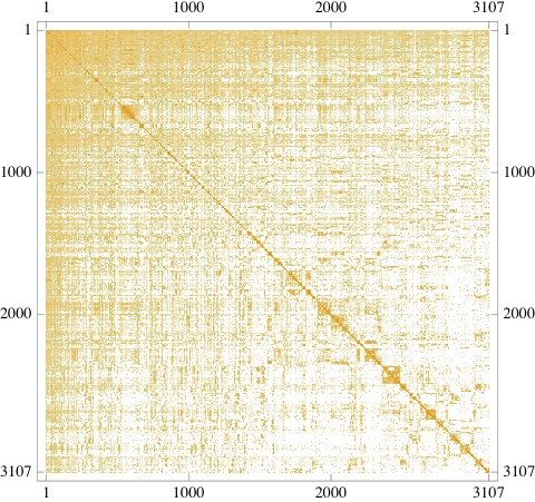
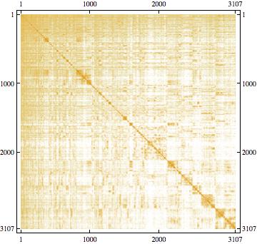
Based upon the 2000 United States Decennial Census, one can construct a square (origin-destination) matrix of 1995-2000 migration flows () between 3,107 county-level units of the nation. In Fig. 1, we show a matrix plot of this (raw data) table. (In the absence of any further relevant information, we set to zero the diagonal entries–which conceptually might correspond either to the number of people who actually moved within the county or who simply stayed within it.) In the principal, admininstrative sorting of the rows/columns of the table, the fifty states are ordered alphabetically, while, secondarily, within the states, their constituent counties are ordered also alphabetically.
We immediately discern a clear clustering along the diagonal in Fig. 1, indicative of the obvious proposition that migrants have a proclivity to move intrastate-wise, both for simple distance and state loyalty/ties/allegiance considerations. However, the alphabetical ordering by states is certainly highly fortuitous in character, and we observe relatively heavy migration far removed from the diagonal (say for the physically contiguous, but alphabetically non-proximate pairs [California, Oregon] and [Texas, Lousiana].) (Historically, the design and layout of counties differs considerably–somewhat unfortunately from a geographic-theoretic point of view–between states, and we note that Texas has the most counties, 254, and appears as a large square far down the diagonal in Fig. 1, while the state of Georgia, with the second most counties, 159, is also apparent near the upper left corner.)
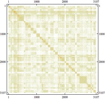
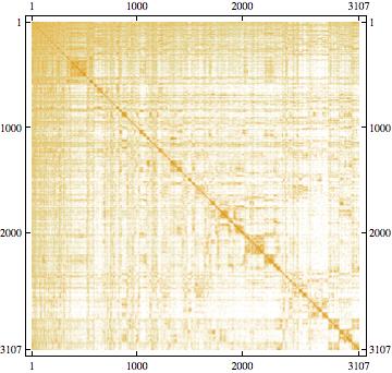
Additionally, counties vary widely in population sizes. To control for this (marginal) effect, one may biproportionally/iteratively adjust the row and column sums so that they all converge to be equal (say to 1). In Fig. 2, we show the intercounty migration table after such a double-standardization (bistochastization). Clearly, the underlying definition/delimitation of blocks has been heightened by this transformation. The purpose of the scaling is to remove overall effects of size (which certainly may be of interest in themselves), and focus on relative, interaction effects. Nevertheless, the cross-product ratios (relative odds), , measures of association, are left invariant. Additionally, the entries of the doubly-stochastic table provide maximum entropy estimates of the original flows, given the constraints on the row and column sums Eriksson (1980); Macgill (1977). Let us also make the general observations that powers of bistochastic matrices are also bistochastic, and that physicists have been interested in developing conditions that indicate when a bistochastic matrix is also unistochastic Louck (1997); Życzkowski et al. (2003); Bengtsson et al. (2005); Diţă (2006). (These latter properties might be of value in the modeling of transaction flows.) An efficient algorithm–considered as a nonlinear dynamical system–to generate random bistochastic matrices has recently been presented Cappellini et al. (cf. Griffiths (1974); Życzkowski et al. (2003)).
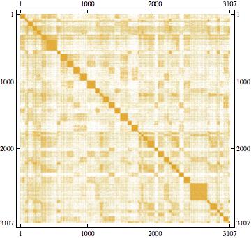
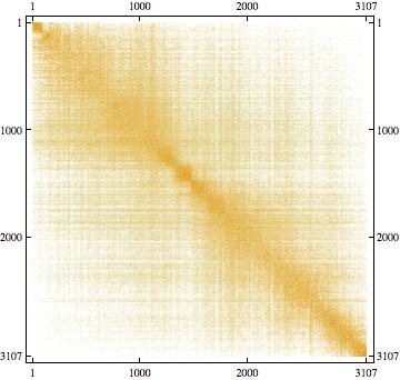
The dominant left and right eigenvectors (corresponding to the eigenvalue 1) of the doubly-standardized table are simply uniform vectors. The subdominant (left and right) eigenvectors (corresponding to a real eigenvalue of 0.906253) are of interest Meila and Pentney (2005). (The correlation between these two eigenvectors is high, 0.971197. The third largest eigenvalue is real also, 0.868784, while the fourth is slightly complex in nature, . The vector of 3,107 eigenvalues has length 12.6472.) We reorder or seriate Fig. 2 on the basis of the left (in-migration) eigenvector and obtain Fig. 3, and on the basis of the right (out-migration) eigenvector and obtain Fig. 4. Now we see diminished clustering far from the diagonal. Further, both of these figures suggest the division of the nation into basically two large clusters.
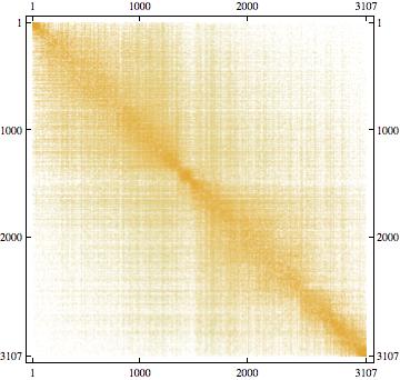
Further, reordering on the basis of the (38-page-long, 3,107-county) dendrogram ((Slater, , Supplement)) generated by the strong component hierarchical clustering (the directed-graph analogue of the single-linkage method) Slater (1976a, 1984a, b, 1983a, 1984b, c, 1981); Tarjan (1982, 1983); Ozawa (1983) of the bistochastized table, we obtain Fig. 5. The correlation between the ordering used in this table and the admininstrative ordering used in Figs. is 0.0373522, and the orderings used in Figs. 3 and 4, respectively, even lower, 0.00401504 and 0.0099957 (Table 1). (The corresponding correlations between the administrative ordering and that employed in Figs. 3 and 4 are 0.0579257 and 0.0755089. Correlations greater in absolute value than 0.0353074 are significant at the level, 0.0400655 at the level, and 0.0458262 at the level.)
| 1 2 | 3 | 4 | 5 | 8 | 9 | |
|---|---|---|---|---|---|---|
| 1 2 | 1. | 0.0579257 | 0.0755089 | 0.0373522 | -0.00868334 | -0.0788444 |
| 3 | 0.0579257 | 1. | 0.140583 | 0.00401504 | 0.00759781 | -0.0202812 |
| 4 | 0.0755089 | 0.140583 | 1. | 0.0099957 | 0.00207526 | -0.000659818 |
| 5 | 0.0373522 | 0.00401504 | 0.0099957 | 1. | 0.0551071 | 0.0206225 |
| 8 | -0.00868334 | 0.00759781 | 0.00207526 | 0.0551071 | 1. | 0.0467724 |
| 9 | -0.0788444 | -0.0202812 | -0.000659818 | 0.0206225 | 0.0467724 | 1. |
The dominant feature of Fig. 5 is that the counties now listed at the beginning in the reordering–and, in general, the last to be absorbed in the agglomerative clustering process–are “cosmopolitan” or “hub-like”. They tend to receive and send migrants across the nation, while those nearer to the end in the reordering tend to be more provincial or limited in their breadth of interactions Slater (1976b). (A prototypical example of a hub-like internal migration area is Paris Slater (1976b); Slater and Winchester (1978). In analytically parallel studies of interjournal citations Slater (1983a); Rosvall and Bergstrom (2008); Bollen et al. (2009), one might anticipate that the broad journals, Science, Nature and the Proceedings of the National Academy of Sciences might fulfill analogous roles.)
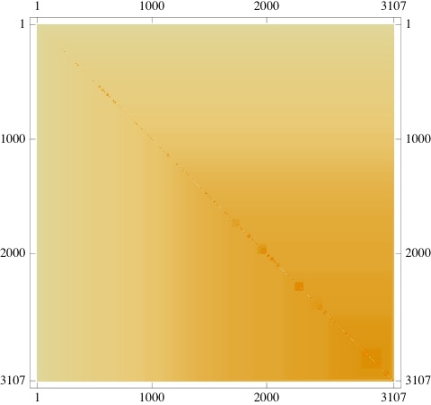
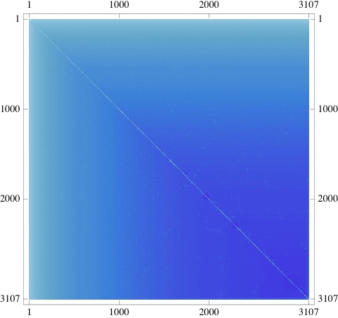
The ultrametric fit to this reordered bistochastized table provided by the strong component hierarchical clustering Slater (1976a, 1984a, b, 1983a, 1984b, c, 1981); Tarjan (1982, 1983); Ozawa (1983) is given in Fig. 6, and the residuals (predominantly negative) from the fit in Fig. 7. (These latter two figures, both in their own ways, further reflect this cosmopolitan-provincial dichotomy between the U. S. counties.) In Fig. 8 we display the bistochastic form of the 1995-2000 U. S. intercounty migration table now reordered on the basis of the hierarchical clustering generated by application of the DirectAgglomerate command of Mathematica. (We inputted our asymmetric values–converted to dissimilarity measures–even though the command assumes a symmetric input. We also applied the same command to the transpose of the dissimilarity matrix, and obtained somewhat differing results [Fig. 9].) The correlation between the orderings in Fig. 8 and Fig. 9 is 0.0467724, and that of the ordering in Fig. 5 with those in Figs. 8 and 9, 0.0551071 and 0.0206225, respectively. (With the administrative ordering used in Figs. 1 and 2, the correlations with Figs. 8 and 9 are negative, -0.00868334 and [negatively significant] -0.078844, respectively.)
Previously Slater (1983b, 1981), we have studied (without the aid of more recently-developed matrix plots) bistochastized forms of the 1965-70 U. S. intercounty migration table with strong component hierarchical clustering Slater (1976a, 1984a, b, 1983a, 1984b, c, 1981); Tarjan (1982, 1983); Ozawa (1983), both with zero and non-zero (corresponding to intracounty movements) diagonal entries. Counties with large physical areas tend to absorb more of their own migrants, and thus exhibit larger diagonal bistochasticized entries and smaller off-diagonal entries, making them link at weaker levels in the dendrogram generated. Journals with high self-citations would be expected to behave analogously in journal citation-matrix analyses Slater (1983a); Rosvall and Bergstrom (2008); Leydesdorff (2004). In the application of our two-stage bistochastization and strong component hierarchical clustering procedure to the 1967-75 interjournal citations between twenty-two mathematical journals, the Proceedings of the American Mathematical Society was found to function in a particularly broad, cosmopolitan manner Slater (1983a).
Acknowledgements.
I would like to express appreciation to the Kavli Institute for Theoretical Physics (KITP) for technical support.References
- Eriksson (1980) J. Eriksson, Math. Program. 18, 146 (1980).
- Macgill (1977) S. M. Macgill, Environ. Plann. A 9, 687 (1977).
- Życzkowski et al. (2003) K. Życzkowski, M. Kuś, W. Słomczyński, and H.-J. Sommers, J. Phys. A 36, 3425 (2003).
- Bengtsson et al. (2005) I. Bengtsson, Ȧ. Ericsson, M. Kús, W. Tadej, and K. Życzkowski, Commun. Math. Phys. 259, 307 (2005).
- Diţă (2006) P. Diţă, J. Math. Phys. 47, 083510 (2006).
- Louck (1997) J. D. Louck, Found. Phys. 27, 1085 (1997).
- (7) V. Cappellini, H.-J. Sommers, W. Bruzda, and K. Życzkowski, Nonlinear dynamics in constructing random bistochastic matrices, eprint arXiv:0711.3345.
- Griffiths (1974) R. C. Griffiths, Canad. J. Math. 26, 600 (1974).
- Meila and Pentney (2005) M. Meila and W. Pentney, in Proc. Natl. Conf. Artificial Intelligence (2005).
- (10) P. B. Slater, Hubs and clusters in the evolving U. S. intercounty migration network, eprint arXiv:0809.2768.
- Slater (1976a) P. B. Slater, Regional Stud. 10, 123 (1976a).
- Slater (1984a) P. B. Slater, Tree representations of internal migration flows and related topics (Community and Organization Res. Inst., Santa Barbara, 1984a).
- Slater (1976b) P. B. Slater, IEEE Syst. Man. Cyb. 6, 321 (1976b).
- Slater (1983a) P. B. Slater, Scientometrics 5, 55 (1983a).
- Slater (1984b) P. B. Slater, Environ. Plann. A 16, 545 (1984b).
- Slater (1976c) P. B. Slater, Rev. Public Data Use 4, 32 (1976c).
- Slater (1981) P. B. Slater, Quality and Quantity 15, 179 (1981).
- Tarjan (1982) R. E. Tarjan, Info. Proc. Lett. 14, 26 (1982).
- Tarjan (1983) R. E. Tarjan, Info. Proc. Lett. 17, 37 (1983).
- Ozawa (1983) K. Ozawa, Patt. Recog. 16, 201 (1983).
- Slater and Winchester (1978) P. B. Slater and H. L. M. Winchester, IEEE Syst. Man. Cyb. 8, 635 (1978).
- Rosvall and Bergstrom (2008) M. Rosvall and C. T. Bergstrom, Proc. Natl. Acad. Sci. 105, 1118 (2008).
- Bollen et al. (2009) J. Bollen, H. Sompel, A. Hagberg, L. Bettancourt, R. Chute, and L. Balakireva, PLoS One 4, e4803 (2009).
- Slater (1983b) P. B. Slater, Migration regions of the United States: two county-level 1965-70 analyses (Community and Organization Res. Inst., Santa Barbara, 1983b).
- Leydesdorff (2004) L. Leydesdorff, Scientometrics 60, 159 (2004).