Abstract

In this manuscript we give thought to the aftermath on the stable probability density function when standard multiplicative cascades are generalised cascades based on the $q$-product of Borges that emerged in the context of non-extensive statistical mechanics.

1 Introduction

In the twenty years that have elapsed since the publication of the non-additive entropy $S_{q}$, also fairly known as Tsallis entropy [1], many applications and connections to natural and man-mind phenomena have been established [2]. One of the most exciting which that have emerged within the non-extensive scope is the definition of a whole new set of mathematical operations/functions that goes from the generalised algebra independently defined by Borges [3] and Nivanen et al. [4] and the integro-differential operators by Borges to the $q$-trigonometric functions [5]. Besides its inherent beauty, these generalisations have found its own field of applicability. Namely, the $q$-product plays a primary role in the definition of the $q$-Fourier transform [6], thus in $q$-Central Limit Theorem [7], whereas the generalised trigonometric functions have been quite successful in describing the critical behaviour of a class of composed materials known as manganites [8]. In this article, we inquire into the possible applications of the $q$-product in the generation of random variables and its consequence on the definition of a new class of probability density functions.

2 Preliminaries: the $q$-product

The $q$-product, $\otimes_{q}$, has been introduced with the purpose to find a functional form that is able to generalise in a non-extensive way the mathematical identity,

$$\exp\left[\ln\,x+\ln\,y\right]=x\times y,\qquad\left(x,y>0\right),$$ (1)

so that the equality,

$$x\otimes_{q}y\equiv\exp_{q}\left[\ln_{q}\,x+\ln_{q}\,y\right],$$ (2)

holds. The representations $\ln_{q}\left(.\right)$ and $\exp_{q}\left(.\right)$ correspond to the $q$-logarithm [9],

$$\ln_{q}\left(x\right)\equiv\frac{x^{1-q}-1}{1-q},\qquad\left(x>0,q\in\Re\right),$$ (3)

and its inverse, the $q$-exponential,

$$\exp_{q}\left(x\right)\equiv\left[1+\left(1-q\right)\,x\right]^{\frac{1}{1-q}},\qquad\left(x,q\in\Re\right),$$ (4)

respectively ($\exp_{q}\left(x\right)=0$ if $1+(1-q)\,x\leq 0$). For $q\rightarrow 1$, the equation (2) recovers the usual property,

$$\ln\left(x\times y\right)=\ln\,x+\ln\,y$$

($x,y>0$), with $x\times y\equiv x\otimes_{1}y$. Its inverse operation, the $q$-division, $x\oslash_{q}y$, verifies the following equality $\left(x\otimes_{q}y\right)\oslash_{q}y=x$.

Bearing in mind that the $q$-exponential is a non-negative function, the $q$-product must be restricted to the values of $x$ and $y$ that respect the condition,

$$\left|x\right|^{1-q}+\left|y\right|^{1-q}-1\geq 0.$$ (5)

Moreover, we can extend the domain of the $q$-product to negative values of $x$ and $y$ writing it as,

$$x\otimes_{q}y\equiv\mathrm{\ sign}\left(x\,y\right)\exp_{q}\left[\ln_{q}\,\left|x\right|+\ln_{q}\,\left|y\right|\right].$$ (6)

Regarding some key properties of the $q$-product we mention:

1. $x\otimes_{1}y=x\ y$;

2. $x\otimes_{q}y=y\otimes_{q}x$;

3. $\left(x\otimes_{q}y\right)\otimes_{q}z=x\otimes_{q}\left(y\otimes_{q}z\right)=\left[x^{1-q}+y^{1-q}-2\right]^{\frac{1}{1-q}}$;

4. $\left(x\otimes_{q}1\right)=x$;

5. $\ln_{q}\left[x\otimes_{q}y\right]\equiv\ln_{q}\,x+\ln_{q}\,y$;

6. $\ln_{q}\left(x\,y\right)=\ln_{q}\left(x\right)+\ln_{q}\left(y\right)+\left(1-q\right)\ln_{q}\left(x\right)\ln_{q}\left(y\right)$;

7. $\left(x\otimes_{q}y\right)^{-1}=x^{-1}\otimes_{2-q}y^{-1}$;

8. $\left(x\otimes_{q}0\right)=\left\{\begin{array}[]{ccc}0&&\mathrm{if\ }\left(q\geq 1\ \mathrm{and\ }x\geq 0\right)\ \mathrm{or\ if\ }\left(q<1\ \mathrm{and\ }0\leq x\leq 1\right)\\ &&\\ \left(x^{1-q}-1\right)^{\frac{1}{1-q}}&&\mathrm{otherwise}\end{array}\right.$

For particular values of $q$, e.g., $q=1/2$, the $q$-product provides nonnegative values at points for which the inequality $\left|x\right|^{1-q}+\left|y\right|^{1-q}-1<0$ is verified. According to the cut-off of the $q$-exponential, a value of zero for $x\otimes_{q}y$ is set down in these cases. Restraining our analysis of the Eq. (5) to the sub-space $x,y>0$, we can observe that for $q\rightarrow-\infty$ the region $\left\{0\leq x\leq 1,0\leq y\leq 1\right\}$ is not defined. As the value of $q$ increases, the forbidden region decreases its area, and when $q=0$, we have the limiting line given by $x+y=1$, for which $x\otimes_{0}y=0$. Only for $q=1$, the entire set of $x$ and $y$ real values of has a defined value for the $q$-product. For $q>1$, the condition (5) implies a region, $\left|x\right|^{1-q}+\left|y\right|^{1-q}=1$ for which the $q$-product diverges. This undefined region augments its area as $q$ goes to infinity. When $q=\infty$, the $q$-product is only defined in $\left\{x\geq 0,0\leq y\leq 1\right\}\cup\left\{0\leq x\leq 1,y>1\right\}$. Illustrative plots are presented in Fig. (1) of Ref. [10].

3 Multiplicative processes as generators of distributions

Multiplicative processes, particularly stochastic multiplicative processes, have been the source of plenty of models applied in several fields of science and knowledge. In this context, we can name the study of fluid turbulence [11], fractals [12], finance [13], linguistics [14], etc. Specifically, multiplicative processes play a very important role on the emergence of the log-Normal distribution as a natural and ubiquitous distribution. In simple terms, the log-Normal distribution is the distribution of a random variable whose logarithm is associated with a Normal distribution [15],

$$p\left(x\right)=\frac{1}{\sqrt{2\pi}\sigma x}\exp\left[-\frac{\left(\ln x-\mu\right)^{2}}{2\sigma^{2}}\right].$$ (7)

With regard to the dynamical origins of the log-Normal distribution, several processes have been thought up to generate it. In this work we highlight the two most famous — the law of proportionate effect [16], the theory of breakage [17] or from Langevin-like processes [18]. We shall now give a brief view of the former; Let us consider a variable $\tilde{Z}$ obtained from a multiplicative random process,

$$\tilde{Z}=\prod\limits_{i=1}^{N}\tilde{\zeta}_{i},$$ (8)

where $\tilde{\zeta}_{i}$ are nonnegative microscopic variables associated with a distribution $f^{\prime}\left(\tilde{\zeta}\right)$. If we consider the following transform of variables $Z\equiv\ln\tilde{Z}$, then we have,

$$Z=\sum\limits_{i=1}^{N}\zeta_{i},$$

with $\zeta\equiv\ln\tilde{\zeta}$. Assume now $\zeta$ as a variable associated with a distribution $f\left(\zeta\right)$ with average $\mu$ and variance $\sigma^{2}$. Then, $Z$ converges to the Gaussian distribution in the limit of $N$ going to infinity as entailed by the Central Limit Theorem [19]. Explicitly, considering that the variables $\zeta$ are independently and identically distributed, the Fourier Transform of $p\left(Z^{\prime}\right)$ is given by,

$$\mathcal{F}\left[p\left(Z^{\prime}\right)\right]\left(k\right)=\left[\int_{-\infty}^{+\infty}e^{i\,k\,\frac{\zeta}{N}}\,f\left(\zeta\right)\,d\zeta\right]^{N},$$ (9)

where $Z^{\prime}=N^{-1}Z$. For all $N$, the integrand can be expanded as,

$$\begin{array}[]{c}\mathcal{F}\left[p\left(Z^{\prime}\right)\right]\left(k\right)=\left[\sum\limits_{n=0}^{\infty}\frac{\left(ik\right)^{n}}{n!}\frac{\left\langle\zeta^{n}\right\rangle}{N}\right]^{N},\\ \\ \mathcal{F}\left[p\left(Z^{\prime}\right)\right]\left(k\right)=\exp\left\{N\ln\left[1+ik\frac{\left\langle\zeta\right\rangle}{N}-\frac{1}{2}k^{2}\frac{\left\langle\zeta^{2}\right\rangle}{N^{2}}+O\left(N^{-3}\right)\right]\right\},\end{array}$$ (10)

expanding the logarithm,

$$\mathcal{F}\left[P\left(Z^{\prime}\right)\right]\left(k\right)\approx\exp\left[ik\mu-\frac{1}{2N}k^{2}\sigma^{2}\right].$$ (11)

Applying the inverse Fourier Transform, and reverting the $Z^{\prime}$ change of variables we finally obtain,

$$p\left(Z\right)=\frac{1}{\sqrt{2\,\pi\,N}\sigma}\exp\left[-\frac{\left(Z-N\,\mu\right)^{2}}{2\,\sigma^{2}\,N}\right].$$ (12)

We can define the attracting distribution in terms of the original multiplicative random process, yielding the log-Normal distribution [15],

$$p\left(\bar{Z}\right)=\frac{1}{\sqrt{2\,\pi\,N}\sigma\,\bar{Z}}\exp\left[-\frac{\left(\ln\bar{Z}-N\,\mu\right)^{2}}{2\,\sigma^{2}\,N}\right].$$ (13)

Although this distribution with two parameters, $\mu$ and $\sigma$, is able to appropriately describe a large variety of data sets, there are cases for which the log-Normal distribution fails statistical testing [15]. In some of these cases, such a failure has been overcome by introducing different statistical distributions (e.g., Weibull distributions) or changing the 2-parameter log-Normal distribution by a 3-parameter log-Normal distribution,

$$p\left(x\right)=\frac{1}{\sqrt{2\,\pi}\sigma\,\left(x-\theta\right)}\exp\left[-\frac{\left(\ln\left[x-\theta\right]-\mu\right)^{2}}{2\,\sigma^{2}}\right].$$ (14)

In the sequel of this work we present an alternative procedure to generalise the Eq. (7). The motivation for this proposal comes from changing the $N$ products in Eq. (8) by $N$ $q$-products,

$$\tilde{Z}=\underset{}{\prod\limits_{i=1}^{N}}^{(q)}\tilde{\zeta}_{i}\equiv\tilde{\zeta}_{1}\otimes_{q}\tilde{\zeta}_{2}\otimes_{q}\ldots\otimes_{q}\tilde{\zeta}_{N}.$$ (15)

Applying the $q$-logarithm we have a sum of $N$ terms. If every term is identically and independently distributed, then for variables $\zeta_{i}=\ln_{q}$ $\tilde{\zeta}_{i}$ with finite variables we have a Gaussian has stable distribution, i.e., a Gaussian distribution in the $q$-logarithm variable. From this scenario we can obtain our $q$-log Normal probability density function,

$$p\left(x\right)=\frac{1}{\mathcal{Z}_{q}\,x^{q}}\exp\left[-\frac{\left(\ln_{q}\,x-\mu\right)^{2}}{2\,\sigma^{2}}\right],\qquad\left(x\geq 0\right),$$ (16)

with the normalisation,

$$\mathcal{Z}_{q}=\left\{\begin{array}[]{ccc}\sqrt{\frac{\pi}{2}}\mathrm{erfc}\left[-\frac{1}{\sqrt{2}\sigma}\left(\frac{1}{1-q}+\mu\right)\right]\sigma&if&q<1\\ &&\\ \sqrt{\frac{\pi}{2}}\mathrm{erfc}\left[\frac{1}{\sqrt{2}\sigma}\left(\frac{1}{1-q}+\mu\right)\right]\sigma&if&q>1.\end{array}\right.$$ (17)

In the limit of $q$ equal to $1$, $\ln_{q\rightarrow 1}x=\ln x$ and $\mathcal{Z}_{q\rightarrow 1}=\sqrt{2\,\pi}\sigma$ and the usual log-Normal is recovered thereof (erfc stands for complementary error function). Typical plots for cases with $q=\frac{4}{5}$, $q=1$, $q=\frac{5}{4}$ are depicted in Fig. 1.

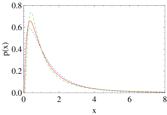
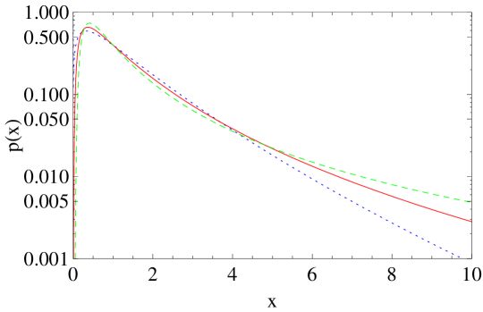
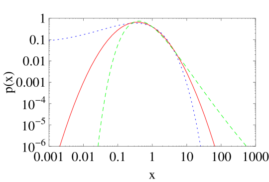
Figure 1: Plots of the Eq. (16) vs $x$ for $q=\frac{4}{5}$ (dotted line), $q=1$ (full line) and $q=\frac{5}{4}$ (dashed line) in linear-linear scale (upper), log-linear (centre), log-log (lower).

The raw statistical moments,

$$\left\langle x^{n}\right\rangle\equiv\int_{0}^{\infty}x^{n}\,p\left(x\right)\,dx,$$ (18)

can be analytically computed for $q<1$ giving [20],

$$\left\langle x^{n}\right\rangle=\frac{\Gamma\left[\nu\right]\exp\left[-\frac{\gamma^{2}}{8\,\beta}\right]D_{-\nu}\left[\frac{\gamma}{\sqrt{2\,\beta}}\right]}{\sqrt{\beta^{\nu}\,\pi}\sigma\left(1-q\right)\mathrm{erfc}\left[-\frac{1}{\sqrt{2}\sigma}\left(\frac{1}{1-q}+\mu\right)\right]},$$ (19)

with

$$\beta=\frac{1}{2\sigma^{2}\left(1-q\right)^{2}};\quad\gamma=-\frac{1+\mu\,\left(1-q\right)}{\left(1-q\right)^{2}\,\sigma^{2}};\quad\nu=1+\frac{n}{1-q},$$ (20)

where $D_{-a}\left[z\right]$ is the parabolic cylinder function [21]. For $q>1$, the raw moments are given by an expression quite similar to the Eq. (19) with the argument of the erfc replaced by $\frac{1}{\sqrt{2}\sigma}\left(\frac{1}{1-q}+\mu\right)$. However, the finiteness of the raw moments is not guaranteed for every $q>1$ for two very related reasons. First, according to the definition of $D_{-\nu}\left[z\right]$, $\nu$ must be greater than $0$. Second, the core of the probability density function, $\exp\left[-\frac{\left(\ln_{q}\,x-\mu\right)^{2}}{2\,\sigma^{2}}\right]$, does not vanish in the limit of $x$ going to infinity $\infty$,

$$\lim_{x\rightarrow\infty}\exp\left[-\frac{\left(\ln_{q}\,x-\mu\right)^{2}}{2\,\sigma^{2}}\right]=\exp\left[-\frac{\gamma^{2}}{2}\right].$$ (21)

This means that the limit $p\left(x\rightarrow\infty\right)=0$ is introduced by the normalisation factor $x^{-q}$, which comes from redefining the Gaussian of variables,

$$y\equiv\ln_{q}x,$$ (22)

as a distribution of variables $x$. Because of that, if the moment surpasses the value of $q$, then the integral (18) diverges.

4 Examples of cascade generators

In this section, we discuss the upshot of two simple cases in which the dynamical process described in the previous section is applied. We are going to verify that the value of $q$ influences the nature of the attractor in probability space.

4.1 Compact distribution $[0,b]$

Let us consider a compact distribution for indentically and independently distributed variables $x$ within the interval $0$ and $b$. Following what we have described in the preceding section, we can transform our generalised multiplicative process into a simple additive process of $y_{i}$ variables which are now distributed in conformity with the distribution,

$$p^{\prime}\left(y\right)=\frac{1}{b}\left[1+\left(1-q\right)y\right]^{\frac{q}{1-q}},$$ (23)

with $y$ defined between $\frac{1}{q-1}$ and $\frac{b^{1-q}-1}{1-q}$ if $q<1$, whereas $y$ ranges over the interval between $-\infty$ and $\frac{b^{1-q}-1}{1-q}$ when $q>1$. Some curves for the special case $b=2$ are plotted in Fig. 2.

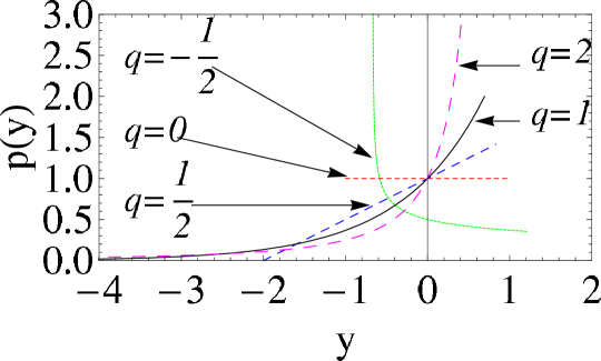
Figure 2: Plots of the Eq. (23) vs $y$ for $b=2$ and the values of $q$ presented in the text.

If we look at the variance of this independent variable,

$$\sigma_{y}^{2}=\left\langle y^{2}\right\rangle-\left\langle\mu_{y}\right\rangle^{2},$$ (24)

which is the moment whose finitude plays the leading role in the Central Limit Theory, we verify that for $q>\frac{3}{2}$, we obtain a divergent value,

$$\sigma_{y}^{2}=\frac{b^{2-2\,q}}{\left(3-2\,q\right)\left(2-q\right)^{2}}.$$ (25)

Hence, if $q<\frac{3}{2}$, we can apply the Lyapunov’s central Limit theorem and our attractor in the probability space is the Gaussian distribution. On the other hand, if $q>\frac{3}{2}$, the Lévy-Gnedenko’s version of the central limit theorem [22] asserts that the attracting distribution is a Lévy distribution with a tail exponent,

$$\alpha=\frac{1}{q-1}.$$ (26)

Furthermore, it is simple to verify that the interval $\left(\frac{3}{2},\infty\right)$ of $q$ values maps onto the interval $\left(0,2\right)$ of $\alpha$ values, which is precisely the interval of validity of the Lévy class of distributions that is defined by its Fourier Transform,

$$\mathcal{F}\left[L_{\alpha}\left(Y\right)\right]\left(k\right)=\exp\left[-a\,\left|k\right|^{\alpha}\right].$$ (27)

In Fig. 3 we depict some sets generated by this process for different values of $q$.

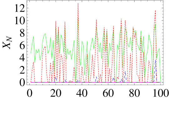
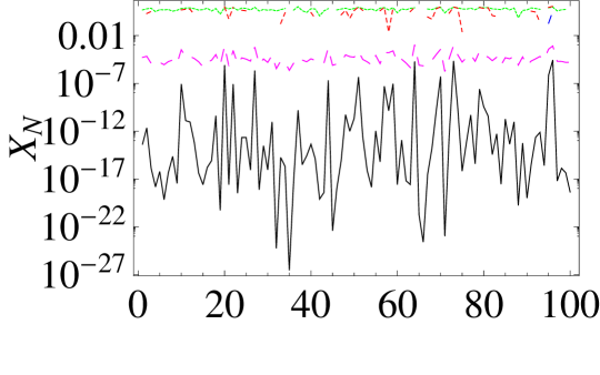
Figure 3: Sets of random variables generated from the process (15) with $N=100$ and $q=-\frac{1}{2}$ (green), $0$ (red), $\frac{1}{2}$ (blue), $1$ (black), $\frac{5}{4}$ (magenta) in linear (upper panel) and log scales (lower panel). The generating variable is uniformly distributed within the interval $\left[0,1\right]$ as is the same for all of the cases that we present. As visible, the value of $q$ deeply affects the values of $X_{N}=\tilde{Z}$.

4.2 $q$-log Normal distribution

In this example, we consider the case of generalised multiplicative processes in which the variables follow a $q$-log Normal distribution. In agreement with what we have referred to in Sec. 3, the outcome strongly depends on the value of $q$. Consequently, in the associated $x$ space, if we apply the generalised process to $N$ variables $y=\ln_{q}\,x$ ($x\in\left[0,\infty\right)$) which follow a Gaussian-like functional form with average $\mu$ and finite standard deviation $\sigma$, i.e., $\forall_{q<1}$ or $q>3$ in Eq.(16), the resulting distribution in the limit of $N$ going to infinity corresponds to the probability density function (16) with $\mu\rightarrow N\,\mu$ and $\sigma^{2}\rightarrow N\,\sigma^{2}$. In respect of the conditions of $q$ we have just mentioned here above, the $q$-log normal can be seen as an asymptotic attractor, a stable attractor for $q=1$, and an unstable distribution for the remaining cases with the resulting attracting distribution being computed by applying the convolution operation.

5 Final remarks

In this manuscript we have introduced a modification in the multiplicative process that has enabled us to present a modification on the log-Normal distribution as well as other distributions with slow decay. This distribution is controlled by an extra-parameter, $q$, when it is compared with the regular 2-parameter log-Normal distribution, that can be dynamically related to a change in the multiplicative random process. Besides, it provides interesting mechanisms of on-off dynamics.

Regarding further applications, it is known that the standard log-normal distribution is unfitted for several data sets. This 3-parameter log-Normal probability function is expected to provide a better approach to these data [23].

SMDQ thanks his colleagues at Unilever for discussions and financial support of the Marie Curie Fellowship programme (European Union).

References

- [1] C. Tsallis, J. Stat. Phys. 52, 479 (1988)
- [2] C. Tsallis, Introduction to Nonextensive Statistical Mechanics: Approaching a Complex World (Springer, Berlin, 2009);Complexity, Metastability, and Nonextensivity: An International Conference edited by S. Abe, H. Herrmann, P. Quarati, A. Rapisarda, C. Tsallis, AIP Conf. Proc. 965 (2007); Complexity, Metastability and Nonextensivity, edited by C. Beck, G. Benedek, A. Rapisarda, C. Tsallis (World Scientific, Singapore, 2005); Nonextensive Entropy – Interdisciplinary Applications, edited by M. Gell-Mann, C. Tsallis (Oxford University Press, New York, 2004)
- [3] E.P. Borges, Physica A 340, 95 (2004)
- [4] L. Nivanen, A. Le Mehaute and Q.A. Wang, Rep. Math. Phys. 52, 437 (2003)
- [5] E.P. Borges, Doctorate Thesis, CBPF, Rio de Janeiro (unpublished, 2004) [in Portuguese].
- [6] S. Umarov, and C. Tsallis, Phys. Lett. A 372, 4874-4876 (2008); S. Umarov, S.M. Duarte Queirós, e-print arXiv:0711.2550 [cond-mat.stat-mech] (preprint, 2008)
- [7] S. Umarov, C. Tsallis, S. Steinberg, Milan J. Math, ;S. Umarov and C. Tsallis, Complexity, Metastability, and Nonextensivity: An International Conference edited by S. Abe, H. Herrmann, P. Quarati, A. Rapisarda, C. Tsallis, AIP Conf. Proc. 965, 34 (2007); S. Umarov, C. Tsallis, M. Gell-Mann and S. Steinberg, e-print arXiv:cond-mat/0606040 [cond-mat.stat-mech] (preprint, 2006) and e-print arXiv:cond-mat/0606038 [cond-mat.stat-mech] (preprint, 2006)
- [8] M.S. Reis, J.C.C. Freitas, M.T.D. Orlando, E.K. Lenzi and I.S. Oliveira, Europhys. Lett. 58, 42 (2002)
- [9] C. Tsallis, Quimica Nova 17, 468 (1994)
- [10] S.M. Duarte Queirós and C. Tsallis, Complexity, Metastability, and Nonextensivity: An International Conference edited by S. Abe, H. Herrmann, P. Quarati, A. Rapisarda, C. Tsallis, AIP Conf. Proc. 965, 8 (2007);
- [11] U. Frisch, Turbulence: The Legacy of A. Kolmogorov (Cambridge University Press, Cambridge, 1997); C. Beck, E.G.D Cohen, and H.L. Swinney, Phys. Rev. E 72, 056133 (2005)
- [12] J. Feder, Fractals (Plenum, New York, 1988)
- [13] B.B. Mandelbrot, Fractals and Scaling in Finance (Springer, New York, 1997)
- [14] D. Stauffer, S.M. Moss de Oliveira, P.M.C. de Oliveira and J.M. de Sá Martins, Biology, Sociology, Geology by Computational Physicists, Vol. 1 (Elsevier, Amsterdam, 2006)
- [15] Lognormal Distributions: Theory and Applications, edited by E.L. Crow and K. Shimizu (CRC Pess, New York, 1988)
- [16] R. Gibrat, Bull. Statist. Gén. Fr. 19, 469 (1930)
- [17] A.N. Kolmogorov, Dok. Acad. Nauk SSSR 31, 99 (1941)
- [18] K.S. Fa, Chem. Phys. 287, 1 (2003)
- [19] A. Araujo, E. Guiné, The Central Limit Theorem for Real and Banach Valued Random Variables (John Wiley & Sons, New York, 1980)
- [20] I.S. Gradshteyn and I.M. Ryzhik, Table of Integrals, Series, and Products (Academic Press, New York, 1980), 3.462.1
- [21] http://functions.wolfram.com/HypergeometricFunctions/ ParabolicCylinderD/
- [22] P. Lévy, Théorie de I’addition des variables aléatoires (Gauthierr-Villards, Paris, 1954)
- [23] S.M. Duarte Queirós, Unilever R&D Port Sunlight Internal Report No PS 09 0010 (unpublished, 2009).