Kondo Lattice Scenario in Disordered Semiconductor Heterostructures

Abstract

We study nuclear relaxation in the presence of localized electrons in a two-dimensional electron gas in a disordered delta-doped semiconductor heterostructure and show that this method can reliably probe their magnetic interactions and possible long-range order. In contrast, we argue that transport measurements, the commonly-employed tool, may not sometimes distinguish between spatial disorder and long-range order. We illustrate the utility of using the nuclear relaxation method to detect long-range order by analysing a recent proposal made on the basis of transport measurements, on the spontaneous formation of a two-dimensional Kondo lattice in a 2D electron gas in a heterostructure.

Introduction- The possibility of long-range charge or magnetic order of strongly-correlated electrons in mesoscopic devices, such as Wigner crystals bello ; grill , charge density waves willett , and Kondo lattices siegert , has attracted a great deal of attention in recent times. Theoretical interest in these systems stems from the low-dimensionality which enhances quantum effects, while the practical motivation comes from the tunability of the material parameters by electrical means, which is not achievable in bulk materials. Experimental probes for long-range order in mesoscopic devices have been usually based on transport measurements siegert as their small size makes it difficult to employ standard bulk methods such as diffraction and nuclear magnetic resonance (NMR)alloul-kondo ; boyce-kondo ; ross-CDW . However suitably adapted NMR methods are now beginning to emerge as very promising tools for studying electron interactions in mesoscopic systems – recent work shows that nuclear polarization may be generated yusa ; wald ; dixon ; machida ; tripathi-rashba locally in such devices and its relaxation can be feasibly detected cooper ; nesteroff through two-terminal conductance measurements, and the behavior of the nuclear relaxation rate conveys useful information about the electronic state in the device. For example in the context of the decade-old puzzle of the $0.7$ conductance anomaly in quantum point-contact devices thomas , NMR can be used to distinguish between three incompatible contesting theories - a Kondo effect, a spin-incoherent Luttinger liquid state, or a polarized electron liquid cooper even though transport properties are similar in the three scenarios.

In this paper, we study nuclear relaxation as a probe for long-range magnetic (and crystalline) order of localized spins in a disordered, metallic two-dimensional electron gas (2DEG) in a delta-doped heterostructure. We find that the temperature dependence of the relaxation rate for a disordered few-impurity system approximately follows a linear$-T$ law, while for strong enough inter-spin interactions, nuclear relaxation in a regular array, or a Kondo lattice, will show an exponential increase, $e^{A/T},$ with decreasing temperature. In contrast, we argue that transport measurements will show no significant difference between the two situations. As an application of our analysis, we discuss a recent experimental claim siegert based on transport measurements in disordered GaAs/AlGaAs delta-doped heterostructures, on the spontaneous formation of a Kondo lattice in the 2D electron gas in the heterostructure.

Experimental context- Kondo lattice materials, such as heavy fermion metals, are being intensely studied gegenwart ; schroeder to understand the nature of the competition of the magnetic ordering tendency of the localized electrons and the screening tendency (Kondo effect) of the conduction electrons, close to quantum criticality. A 2D Kondo lattice, if engineered in a heterotructure, would offer the twin advantages of reduced dimensionality and tunability of parameterssiegert , and, as we show below, nuclear relaxation can be used to study these systems.

In Ref. siegert it was observed that the 2DEG conductance showed an alternating splitting and merging of a zero bias anomaly (ZBA) upon varying the gate voltage $V_{g}.$ The authors interpreted these observations as evidence for the formation of a spin-1/2 Kondo lattice embedded in a 2DEG with the following physical picture. Varying the gate voltage affects the 2DEG density, which, in turn, controls the sign of the RKKY exchange interaction, $J_{RKKY}(R_{ij})\sim(J^{2}\rho/R_{ij}^{2})\cos(2k_{F}R_{ij}),$ of the localized spins. Here $J$ is the Kondo coupling of the localized spins with the conduction electrons, and $\rho$ is the density of states at the Fermi energy.

Nevertheless, the observation of the ZBA splitting is not sufficient to prove the existence of a Kondo lattice. Such an effect has been observed in the context of double quantum dot (DQD) systems jeong ; lopez-aguado , and attributed to the competition of Kondo and interdot exchange interactions. Even in a sample with a small number of localized spins, the Kondo and RKKY competition will be dominated by the pairs of spins with the strongest exchange interactions. To this end, we need to show that the nuclear relaxation rates have qualitatively different signatures for the Kondo lattice and few Kondo impurities scenarios.

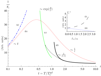
Figure 1: (Color online) Plots showing the qualitative differences in the temperature and (AFM) interdot exchange interaction $J_{\text{ex}}$ dependencies of the nuclear relaxation rates $T_{1}^{-1}$ for a double quantum dot system and Kondo lattice. Main plot: $T_{1}^{-1}(T)$ for (a) a double dot system; (b) a Kondo interaction dominated lattice ($J_{\text{ex}}/\omega_{K}<1$); (c,d) a Kondo lattice where $J_{\text{ex}}/\omega_{K}>1$ and $T<(>)T_{C}^{\text{mf}},$ where $T_{C}^{\text{mf}}$ is the mean-field transition temperature. Dotted curve interpolates between these two temperature regimes (there is no phase transition). Inset: $T_{1}^{-1}$as a function of $J_{\text{ex}}/\omega_{K}$ for (i) the double dot system - note that $T_{1}^{-1}$ vanishes for $J_{\text{ex}}/\omega_{K}>\pi;$ and (ii) for the Kondo lattice.

Nuclear relaxation takes place through nuclear coupling to localized spins $\mathbf{S}$ as well as conduction electrons $\boldsymbol{\sigma}:$ ${\cal H}_{\text{loc}}=A_{d}\mathbf{I}\cdot\mathbf{S}+A_{s}\mathbf{I}\cdot\boldsymbol{\sigma}.$ The relaxation contribution from localized (electron) spins is usually much larger in devices similar to those considered here tripathi-kondo . Taking only the localized spin part, the nuclear relaxation rate can be expressed in terms of the transverse impurity susceptibility, $T_{1}^{-1}=\frac{A_{d}^{2}k_{B}T}{\hbar^{2}(g_{s}\mu_{B})^{2}}\text{Im}\left(\frac{\chi_{i}^{+-}(\omega)}{2\omega}\right)_{\omega\rightarrow 0}.$ We show below that the temperature dependencies of $1/T_{1}$ in the Kondo lattice and few quantum dot scenarios are qualitatively different. The results obtained in the paper are illustrated in Fig. 1 and Table 1.

	FM	AFM
Double impurity	Linear-$T$ at low temp. and $1/T$ at high temp.	Zero at low temp. and $1/T$ at high temp.
Lattice	$T/(T-T_{c})^{3/2}$ at high temp. and $\exp(1/T)$ at low temp.	$T/(T-T_{c})$ at high temp. and $\exp(1/T)$ at low temp.

Table 1: Distinguishing different physical scenarios with NMR

Model- We consider the following model Hamiltonian for $S=1/2$ magnetic impurities ${\mathbf{S}}_{i}$ in a 2-dimensional electron gas:

$$H=\sum_{k}\xi_{k}c_{k\sigma}^{\dagger}c_{k\sigma}+J\sum_{i}\boldsymbol{\sigma}_{i}\cdot\mathbf{S}_{i}.$$ (1)

Here $\boldsymbol{\sigma}_{i}$ the conduction electron spin density at $\mathbf{r}_{i}.$

We use the “drone-fermion” representation for the localized spins Mattis ; Khaliullin : $S_{i}^{+}=f_{i}^{\dagger}\chi_{i}/\sqrt{2},$ $S_{i}^{-}=\chi_{i}f_{i}/\sqrt{2},$ and $S_{i}^{z}=f_{i}^{\dagger}f_{i}-1/2,$ where $f_{i}$ and $f_{i}^{\dagger}$ are ferminonic operators and $\chi$ are real Majorana fermions defined by $\{\chi_{i},\chi_{j}\}=\delta_{ij}$. Note that the commutation relations for the impurity spins are automatically satisfied, obviating the need to impose local constraints on the fermion number. Introducing the bosonic operators, $a_{i}=(f_{i}^{\dagger}c_{i\uparrow}+\chi_{i}c_{i\downarrow}/\sqrt{2})/\sqrt{2},$ $b_{i}=(f_{i}^{\dagger}c_{i\downarrow}^{\dagger}-\chi_{i}c_{i\uparrow}^{\dagger}/\sqrt{2})/\sqrt{2},$ the interaction part of the Hamiltonian (up to constants and irrelevant terms) can be written as $H_{int}=-J\sum_{i}\left(a_{i}^{\dagger}a_{i}+b_{i}^{\dagger}b_{i}\right).$ Factorizing $H_{int}$ using the Hubbard-Stratonovich transformation introducing fields $\Delta_{1}^{i}$ and $\Delta_{2}^{i}$, and further making the transformations $\Delta_{1,2}^{i}=|\Delta_{1,2}^{i}|e^{i\phi_{1,2}^{i}},$ $f\rightarrow fe^{i(\phi_{2}-\phi_{1})},$ $c_{\uparrow}(r)\rightarrow c_{\uparrow}(r)e^{i\phi_{2}},$ $c_{\downarrow}(r)\rightarrow c_{\downarrow}(r)e^{i\phi_{1}},$ the partition function can be written in path integral form:

$${\cal Z} =\int D(c,f,\chi,\Delta)\,e^{-\int_{0}^{\frac{1}{T}}d\tau\left[S_{0}+S_{int}+\frac{1}{J}\sum_{i}\left(|\Delta_{1}^{i}|^{2}+|\Delta_{2}^{i}|^{2}\right)\right]};$$

$$S_{0} =\sum_{k\sigma}c_{k\sigma}^{\dagger}\left(\partial_{\tau}+\xi_{k}\right)c_{k\sigma}+\sum_{i}(f_{i}^{\dagger}\partial_{\tau}f_{i}+\frac{1}{2}\chi_{i}\partial_{\tau}\chi_{i}),$$

$$S_{int} =\sum_{i}|\Delta_{1}^{i}|\>(a_{i}+a_{i}^{\dagger})+|\Delta_{2}^{i}|\>(b_{i}+b_{i}^{\dagger})+\dot{\phi}\>\mbox{terms}.$$ (2)

We make a mean field analysis, neglecting the fluctuations in $\phi$’s and $\Delta$’s. The frequency-dependent local transverse susceptibility at low temperatures $T\ll T_{K}$ can be shown to be Khaliullin

$$\frac{\chi_{i}^{+-}\left(\omega_{m}\right)}{(g_{s}\mu_{B})^{2}}=\langle T_{\tau}S_{i}^{+}(\tau)S_{i}^{-}\left(\tau\prime\right)\rangle_{\omega_{m}} \simeq \frac{2}{\pi\left(|\omega_{m}|+\omega_{K}\right)}.$$ (3)

Here $\omega_{m}$ are bosonic Matsubara frequencies, and $\omega_{K}=D\exp(-4/3\rho J).$ Note that $\omega_{K}$ differs from the correct Kondo temperature, $k_{B}T_{K}\sim De^{-1/(\rho J)}.$ This is an artifact of the mean field approach. An analytic continuation, $\chi_{i}^{+-}(\omega_{m})\rightarrow\chi_{i}^{+-}(\omega)=(g_{s}\mu_{B})^{2}/\pi(-i\hbar\omega+\omega_{Ki}),$ to real frequencies leads to the well-known result $T_{1i}^{-1}=A_{d}^{2}k_{B}T/\pi\hbar\omega_{Ki}^{2}$ for $T\ll\omega_{K}.$

Nuclei may also relax through their hyperfine coupling with conduction electrons. It is easy to see that at low temperatures, the ratio of the nuclear relaxation rates from impurity coupling and conduction electron coupling is $(\omega_{K}^{2}\rho^{2}R_{en}^{4}\pi)^{-1},$ where $R_{en}$ is the electron-nucleus separation. Thus the impurity coupling mechanism dominates as long as $R_{en}<1/\sqrt{\omega_{K}\rho\pi^{1/2}}\approx 160{\rm nm}.$

Double or a few-impurity system- We now consider the impurity spin susceptibility for two spins $\mathbf{S}_{1},\mathbf{S}_{2}$ at $\mathbf{R}=\mathbf{R}_{1},\mathbf{R}_{2}$ which have an exchange interaction $H_{\text{ex}}=J_{\text{ex}}(R_{12})\mathbf{S}_{1}\cdot\mathbf{S}_{2}$ among them. If the wavefunctions of the localized electrons have a significant overlap, then direct exchange would be dominant. Indirect (or RKKY) exchange is more important at larger separations. Here it also becomes important to compare the relative strengths of the RKKY interaction between the impurity spins with the hyperfine interaction of either of the impurities with neighboring nuclei. The RKKY interaction $J_{\text{RKKY}}$ falls off with distance $R_{12}$ not faster than $J_{\text{RKKY}}\sim J^{2}\rho/R_{12}^{2}.$ This should be compared with $A_{d}=A_{s}/l_{\text{loc}}R_{\text{dot}}^{2},$ where $R_{\text{dot}}$ is the size of the quantum dot in the plane of the heterostructure and $l_{\text{loc}}$ is the thickness of the 2DEG. We use the following parameters for a GaAs/AlGaAs heterostructure, $J\rho\sim 1,$ $l_{\text{loc}}\sim 1{\rm nm},$ $R_{\text{dot}}\sim 10{\rm nm},$ $A_{s}=3.8\times 10^{-54}{\rm Jm}^{3},$ and $m=0.063m_{e}.$ Then $J_{\text{RKKY}}\gg A_{d}/N_{\text{nuc}}$ is satisfied if $R_{\text{12}}\ll\sqrt{1/A_{d}\rho}\approx 1{\rm mm},$ and this is true for most devices. Thus the nuclei couple to the RKKY bound pair $\mathbf{S}_{1}+\mathbf{S}_{2}$ rather than the spins separately. The impurity susceptibility now involves both on-site and intersite correlations, and we have, to leading order in inter-impurity interaction for $T\ll T_{K}$,

$$\begin{split}T_{1}^{-1}=\frac{A_{d}^{2}k_{B}T}{\pi\hbar\omega_{K1}^{2}}\left(1+\frac{\omega_{K1}^{2}}{\omega_{K2}^{2}}-\frac{J_{\text{ex}}}{\pi\omega_{K2}}\left(1+\frac{\omega_{K1}}{\omega_{K2}}\right)\right)\end{split}.$$ (4)

When $J_{\text{ex}}/\omega_{K}\geq\pi,$ the nuclear relaxation rate is suppressed to zero: this is the maximum value of $J_{\text{ex}}/\omega_{K}$ for which the behavior is governed by the Kondo screening of the impurity spins. Indeed, even for a large ferromagnetic coupling of the spins, the ground state is a Kondo singlet jones . At antiferromagnetic couplings $J_{\text{ex}}>\pi\omega_{K},$ the ground state is an RKKY singlet which is unable to exchange spins with the nuclei. While our analysis is only to leading order in $J_{\text{ex}},$ more accurate calculations jones based on numerical renormalization group methods have shown that this critical point occurs at $J_{\text{ex}}/k_{B}T_{K}\approx 2.2.$

We discuss now the validity of the mean field treatment. Note that the mean field $\Delta$ corresponds to binding energy of the impurity fermion with the local conduction electron. Ignoring fluctuations of the phase of $\Delta$ results in underestimation of $\omega_{K}$ (see text following Eq. 3 and also Ref. Khaliullin ). Amplitude fluctuations of $\Delta$ may be ignored as long as the Kondo energy dominates inter-impurity exchange, i.e., for small $J_{\text{ex}}/\omega_{K}.$ In fact, the mean field approach is incapable of capturing the physics of the magnetically ordered phase.

With a larger number of spatially disordered impurity spins, one can show that for weak inter-impurity interactions, the nuclear relaxation rates have linear-$T$ behavior with logarithmic factors arising from the random distribution of Kondo temperatures of individual impurities miranda . For strong inter-impurity exchange interactions, we can ignore the Kondo effect to leading order. In that case, it is known that the magnetic susceptibility at low temperatures is dominated by pairs with the weakest exchange interactions bhatt-fisher – this leads to a weakly-increasing susceptibility $e^{C\ln^{1/2}(T_{0}/T)}$ (instead of zero for the double impurity case). Nevertheless, the nuclear relaxation rate is dominated by the linear-$T$ prefactor as the exponential term is weaker than any power law.

Kondo lattice- The main physical difference from the two-impurity case is the existence of low energy magnetic excitations in the lattice for any value of the ratio $J_{\text{ex}}/\omega_{K}.$ As a result, significant nuclear relaxation still occurs for large antiferromagnetic inter-impurity couplings unlike the two-impurity case where it vanishes.

We consider first the scenario where we have a lattice of Kondo impurities with a weak exchange interaction ($J_{\text{ex}}\ll\omega_{K}$) among the neighboring spins. Suppose that $J_{\text{ex}}(\mathbf{q})$ has maximum value at $\mathbf{q}=\mathbf{Q},$ and assume the wavevector dependence in the vicinity of the maximum is $J_{\text{ex}}(\mathbf{Q}+\mathbf{q})=J_{\text{ex}}(\mathbf{Q})-(D_{s}/n_{\text{imp}})a^{2}q^{2},$ where $a$ is the lattice constant of the Kondo array and $D_{s}$ the spin wave stiffness. The random phase approximation (RPA) susceptibility in this momentum region has the form

$$\chi_{\mathbf{Q}+\mathbf{q}}^{+-}(\omega,T) = \frac{(g_{s}\mu_{B})^{2}}{\pi\left(\omega_{sf}\left(T\right)-i\hbar\omega+\frac{D_{s}a^{2}q^{2}}{\pi}\right)},$$ (5)

where $\omega_{sf}\left(T\right)=\frac{(g_{s}\mu_{B})^{2}}{\pi\chi_{i}^{+-}(0,T)}-\frac{J_{\text{ex}}(Q)n_{\text{imp}}}{\pi}.$ A new energy scale $\omega_{sf}(0)=\omega_{K}-J_{\text{ex}}(Q)n_{\text{imp}}/\pi$ appears representing the competition of Kondo and inter-impurity exchange interactions. As $J_{\text{ex}}(Q)n_{\text{imp}}\rightarrow\pi\omega_{K},$ the uniform, static transverse susceptibility tends to diverge signaling a magnetic phase transition. Using the known temperature dependence of the susceptibility of a Kondo impurity, $\chi_{i}^{+-}(0,T)\simeq\chi_{i}(0)(1-Ck_{B}^{2}T^{2}/\omega_{K}^{2}),$($C$ is a constant of order $1$), together with the frequency dependence of $\text{Im}\chi$ from Eq. 5, the nuclear relaxation rate for $k_{B}T\ll\omega_{K}$ turns out to be

$$T_{1}^{-1}=A_{d}^{2}k_{B}T/4\pi^{2}\hbar D_{s}\omega_{sf}(T).$$ (6)

There is a crucial difference between the nuclear relaxation results for the Kondo lattice in Eq. 6 and the two-impurity case. Consider for simplicity $\omega_{K1}=\omega_{K2}=\omega_{K}.$ First, near the transition $J_{\text{ex}}(Q)n_{\text{imp}}/\omega_{K}=\pi,$ $1/T_{1}$ for the Kondo lattice is large and finite, while it tends to vanish for the two-impurity case.

Now we consider the case when localized spin-spin interaction is dominant and neglect the Kondo interaction in the zeroth order. We are particularly interested in the regime close to a magnetic phase transition. The Hamiltonian describing the system would be $H=\sum_{k,\sigma}\xi_{k}c_{k\sigma}^{\dagger}c_{k\sigma}+\sum_{\mathbf{q}}J_{\text{ex}}(\mathbf{q})\mathbf{S}_{\mathbf{q}}\cdot\mathbf{S}_{-\mathbf{q}}+J\sum_{i}\boldsymbol{\sigma}_{i}\cdot\mathbf{S}_{i},$ where $J$ is to be treated now as a perturbation. $J_{\text{ex}}(\mathbf{q})$ represents all exchange processes except indirect exchange (RKKY), $J_{\text{RKKY}}(\mathbf{q},\omega)=J^{2}\sum_{\mathbf{k}}\frac{n_{\mathbf{k}-\mathbf{q}/2}-n_{\mathbf{k}+\mathbf{q}/2}}{\omega+\epsilon_{\mathbf{k}-\mathbf{q}/2}-\epsilon_{\mathbf{k}+\mathbf{q}/2}+i\delta}.$ Thus we may write the effective inter-impurity exchange interaction as $J_{\text{ex}}(q,\omega)=J_{\text{ex}}(q)+J_{\text{RKKY}}(q,\omega).$ where We now Taylor expand the exchange interaction near its extremum, $J_{\text{ex}}(\mathbf{Q}+\mathbf{q})=J_{\text{ex}}(\mathbf{Q})(1-\alpha^{2}q^{2}),$ where $J_{\text{ex}}(\mathbf{Q})\alpha^{2}=(D_{s}/n_{\text{imp}})a^{2}.$ The spin susceptibility near the ordering point is approximately

$$\chi_{\mathbf{Q}+\mathbf{q}}^{+-}(\omega) = \frac{(g_{s}\mu_{B})^{2}}{4k_{B}T_{C}^{\text{mf}}\left\{\alpha^{2}/\xi^{2}+\alpha^{2}q^{2}-i\gamma_{\mathbf{Q}+\mathbf{q}}(\omega)\right\}},$$ (7)

where $\mathbf{Q}$ is the wave vector of ordering, $T_{C}^{\text{mf}}$ is the mean-field magnetic transition temperature, $\xi(T)$ is the magnetic correlation length and $\gamma_{\mathbf{q}}(\omega)$ is the imaginary part of $J_{\text{ex}}(\mathbf{q},\omega)/J_{\text{ex}}(\mathbf{Q}),$ $\gamma_{\mathbf{q}}(\omega)\simeq\pi(J\rho)^{2}\hbar\omega/4J_{\text{ex}}(\mathbf{Q})k_{F}q=\gamma(q)\omega.$ We can now estimate the nuclear relaxation rate. For an antiferromagnetic (AFM) square lattice, the ordering happens at $\mathbf{Q}=(\pi/a,\pi/a).$ Then the relaxation rate at the site of any given impurity is

$$T_{1}^{-1}(T) =\frac{A_{d}^{2}(J\rho)^{2}J_{\text{ex}}(Q)n_{\text{imp}}^{2}}{64\hbar D_{s}^{2}k_{F}Q}\frac{T}{T_{C}^{\text{mf}}}\>\frac{\xi(T)^{2}}{a^{2}}.$$ (8)

Eq. 8 differs from estimates chakravarty of $1/T_{1}$ for Heisenberg antiferromagnets because in our case, the magnon decay is on account of the RKKY coupling of the impurity spins. Similarly for the ferromagnetic (FM) case,

$$T_{1}^{-1}(T) \approx \frac{A_{d}^{2}\pi(J\rho)^{2}J_{\text{ex}}(Q)n_{\text{imp}}}{128\hbar k_{F}aD_{s}^{2}}\frac{T}{T_{C}^{\text{mf}}}\frac{\xi(T)^{3}}{a^{3}}.$$ (9)

The temperature dependencies of the correlation lengths are similar for the AFM and FM cases,

$$\xi(T) \simeq\left\{\begin{array}[]{l}\alpha\sqrt{T_{C}^{\text{mf}}/(T-T_{C}^{\text{mf}})},\qquad T>T_{C}^{\text{mf}},\\ a\exp(2\pi D_{s}^{\prime}/k_{B}T),\qquad T<T_{C}^{\text{mf}},\end{array}\right.$$ (12)

where the low temperature behavior for the antiferromagnet was obtained in Refs. chakravarty ; arovas , and for the ferromagnet from Refs. arovas ; takahashi . $D_{s}^{\prime}\approx 0.18J_{\text{ex}}(\mathbf{Q})n_{\text{imp}}$ is the exact spin wave stiffness at $T=0$ for a 2D (square lattice) Heisenberg magnet. These results also differ from the usually-encountered 3D Kondo lattice systems moriya , because of the qualitative difference in the behavior of $\xi(T)$ at low temperatures.

Finally let us discuss the effect of the Kondo interaction on our results. In presence of inter-impurity exchange interactions, the singular Kondo corrections ($\sim(J\rho)\ln(D/k_{B}T)$) to the gyromagnetic ratio of the impurity spins are modified to $(J\rho)\ln(D/\sqrt{J_{\text{ex}}^{2}+k_{B}^{2}T^{2}})$ tsay . Consequently, the primary effect of Kondo corrections is to decrease the Stoner critical temperature $T_{C}^{\text{mf}}$ as well as the pre-factor in the expressions for the nuclear relaxation rates but the temperature dependence of $T_{1}^{-1}$ does not change significantly. Eqs. 4, 6, 8 and 9 are our main results and are plotted in Fig. 1.

There is also a possibility of a magnetic instability below the Kondo temperature. In this case the ZBA splitting would be smaller than the “heavy fermion” bandwidth, $\omega_{K}$, unlike the above case where the ZBA splitting is larger. As an example, for a Fermi liquid with FM spin fluctuations, results for nuclear relaxation available in the literature hatatani and are similar to our $J_{RKKY}/\omega_{K}>1$ results. The difference will be seen in the magnitude of ZBA splitting relative to $\omega_{K}$.

In summary, we calculated the nuclear relaxation rates $T_{1}^{-1}$ for the Kondo lattice and the few disordered magnetic impurities cases and showed that they have qualitatively different low temperature behaviors: when inter-spin exchange interactions are strong compared to the Kondo energy $\omega_{K},$ the temperature dependence of $T_{1}^{-1}$ for the few-impurity system will follow an approximate linear$-T$ law, while for the Kondo lattice $T_{1}^{-1}$ will show an exponential behviour $e^{A/T}$ at low temperatures. In contrast, we argued that transport measurements siegert in this case may not provide a clinching evidence for the formation of crystalline order (Kondo lattice). The exponential temperature dependence is special to two dimensions and indicates stronger spin fluctuations: a power-law behavior is expected in three dimensions on either side of the transition temperaturemoriya . These results also differ from a 2D Heisenberg magnet because in our case, magnon decay is mediated by conduction electrons. We hope our study will work towards encouraging the use of NMR measurements as an additional handle for studying magnetism and long-range order in low-dimensional conductors.

The authors benefited from discussions with M. Kennett and N. Cooper. K.D. and V.T. thank TIFR for support. V.T. also thanks DST for a Ramanujan Grant [No. SR/S2/RJN-23/2006].

References

- (1) M. S. Bello et al., Sov. Phys. JETP 53, 822 (1981).
- (2) R. Grill and G. H. Döhler, Phys. Rev. B 59, 10769 (1999).
- (3) R. L. Willett et al., Phys. Rev. Lett. 65, 112 (1990).
- (4) C. Siegert et al., Nature Phys. 3, 315 (2007).
- (5) H. Alloul, Physica 84-86 B, 449 (1977).
- (6) J. B. Boyce and C. P. Slichter, Phys. Rev. Lett. 32, 61 (1974).
- (7) J. H. Ross et al., Phys. Rev. Lett. 56, 663 (1986).
- (8) G. Yusa et al., Nature (London) 434, 1001 (2005).
- (9) K. R. Wald et al., Phys. Rev. Lett. 73, 1011 (1994).
- (10) D. C. Dixon et al., Phys. Rev. B 56, 4743 (1997).
- (11) T. Machida et al., Phys. Rev. B 65, 233304 (2002).
- (12) V. Tripathi et al., Europhys. Lett. 81, 68001 (2008).
- (13) N. R. Cooper and V. Tripathi, Phys. Rev. B 77, 245324 (2008).
- (14) J. A. Nesteroff et al., Phys. Rev. Lett. 93,126601 (2004).
- (15) K. J. Thomas et al., Phys. Rev. Lett. 77, 135 (1996).
- (16) For a review see P. Gegenwart et al., Nature Phys. 4, 186 (2008).
- (17) A. Schröder et al., Nature 407, 351 (2000).
- (18) R. Lopez et al., Phys. Rev. Lett. 89, 136802 (2002).
- (19) H. Jeong, et al. Science 293, 2221 (2001).
- (20) R. Bhatt and D. Fisher, Phys. Rev. Lett. 68, 3072 (1992).
- (21) V. Tripathi and N. R. Cooper, J. Phys. Cond. Mat. 20, 164215 (2008).
- (22) D. C. Mattis, The Theory of Magnetism, Harper & Row, New York(1965).
- (23) G. G. Khaliullin, JETP 79 (3), 1994.
- (24) B. A. Jones et al., Phys. Rev. Lett. 61, 125 (1988); C. Jayaprakash et al., Phys. Rev. Lett. 47, 737 (1981).
- (25) E. Miranda et al., Phys. Rev Lett. 78, 290 (1997).
- (26) S. Chakravarty et al., Phys. Rev. B 39, 2344 (1989).
- (27) D. Arovas and A. Auerbach, Phys. Rev. B 38, 316 (1988).
- (28) M. Takahashi, Prog. Theor. Phys. 83, 815 (1989).
- (29) T. Moriya, Prog. Theor. Phys. 28, 371 (1962).
- (30) Y. C. Tsay and M. W. Klein, Phys. Rev. B 7, 352 (1973).
- (31) M. Hatatani and T. Moriya, J. Phys. Soc. Jpn. 64, 3434 (1995).